Article

Research on Bridge Damage Identification Based on WPE-MDS and HTF-SAPSO

School of Civil Engineering and Architecture, Wuhan Institute of Technology, Wuhan 430073, China
*
Author to whom correspondence should be addressed.
Buildings 2022, 12(8), 1089; https://doi.org/10.3390/buildings12081089
Submission received: 16 May 2022 / Revised: 12 July 2022 / Accepted: 19 July 2022 / Published: 25 July 2022

Abstract

:
In recent decades, structural damage identification based on the wavelet analysis method has been widely developed, but it is still confronted with many difficulties, such as large decomposition error and complex data. In order to overcome the shortcomings of analysis based on wavelet, the wavelet packet analysis method is adopted to decompose the acceleration data into wavelet packets, and the frequency band energy value after wavelet packet decomposition (WPE) is taken as the different dimensions of the Mahalanobis distance squared (MDS) in this study, where the MDS value of the same element between different samples is calculated, and the mean value of 30 groups of MDS values for each element is processed. The change rate between the MDS value of the element that exceeds the MDS value in the healthy state and the MDS mean value in the healthy state as the objective function. The combination of weight coefficient and hyperbolic tangent function is used to improve the simulated annealing particle swarm optimization (SAPSO) algorithm, and the improved hyperbolic tangent function-simulated annealing particle swarm optimization (HTF-SAPSO) is used to iteratively calculate the damage severity. The numerical simulation and vibration testing of a steel beam are conducted to verify the identification performance of damage location and the analysis of damage severity by this method, respectively. The numerical model of the experimental I-beam is established based on the MATLAB modeling platform, and the different damage cases are utilized to illustrate the correctness of this study. The different proportions of noise effects are adopted to the numerical simulation analysis, where the correlations between noise effects and MDS value and damage severity are analyzed. In the numerical simulation, although the MDS value increases to different degrees with the increase of the noise ratio, the damage identification result of the damaged element remains mostly constant, which indicates that the influence is negligible. In conclusion, it is feasible to construct the damage index via the combination of WPE and MDS values, the damage location can be judged from whether the MDS value of the element exceeds the threshold, and the HTF-SAPSO algorithm is more efficient and accurate to be adopted in the quantification of the damage severity.

1. Introduction

In the field of structural health monitoring, many environmental excitations are non-stationary random processes, and the frequency components of the response signals vary with time. For this type of non-stationary time-varying signal, we must provide the joint distribution information of time domain and frequency domain in order to clearly describe the local information of structural damage. At this stage, time-frequency analysis methods are widely used because of their advantages of representing the variation of components on different scales of time and frequency [1,2,3]; however, we also undertake the data analysis problem behind a large amount of frequency and time domain information. How to accurately reflect the main information of structural damage and avoid the analysis difficulties caused by the complex and large data is a relevant research topic at this stage.
In the latest research on the application of time-frequency analysis methods for structural damage identification, related scholars have made the following research: Razavi et al. [4] constructed the energy difference between the intact state and the damaged state based on the wavelet packet transform energy, and used a numerical example to verify the applicability of the proposed method; Diao et al. [5] used the energy spectrum under the improved Hilbert-Huang transform to construct the characteristics of structural damage, and used support vector machines and regression algorithms for damage localization and damage degree detection; under the monitoring of a limited number of sensors, a damage localization method based on the multivariate empirical mode decomposition theory is proposed by Sony et al. [6], and the damage localization feature is calculated by calculating the percentage difference of the modal energy of the damaged and undamaged structures. From the above literature, in the time-frequency analysis method, the use of energy as the damage feature is one of the current relevant researches, and the research on the structural damage identification using the frequency domain energy value as the eigenvector under the wavelet packet transform is still developing. In Razavi’s research [4], the damage characteristics are revealed by calculating the energy difference of each component between the intact and damaged states, which not only involves the operation of a large matrix at high latitudes, but also is difficult to reflect the structural damage information and deduce more accurate and specific conclusions by synthesizing the differences of each component, which are also reflected in the author’s research conclusions; Liu et al. [7] used the feature fusion theory to fuse the energy of multiple sensors, and used the classifier trained in the neural network to fuse the energy. It can realize damage diagnosis and evaluation, but its method can only determine the damage degree value within a certain range, and cannot solve the exact damage degree value; Chen et al. [8] used the change rate of node energy distribution as the damage detection index, and only performed damage location and analysis of different damage degrees for a single location, which must be further verified the damage results at different locations; Law et al. [9] used the change of wavelet packet energy distribution to classify the structure but failed to further explore the specific damage degree. Overall, in the method of structural damage identification based on wavelet packet energy characteristics, there are corresponding drawbacks. Additionally, in the case of many node eigenvectors obtained by wavelet packet decomposition, it is likely to appear that the accuracy of the recognition results is not high, and if the number of decomposition scales is reduced, it will inevitably lead to omissions in damage information. Therefore, it becomes extremely necessary to find a data processing method that can reduce the dimension of node energy data and fuse the energy data between nodes.
To overcome the deficiencies brought about by the above wavelet packet energy characteristics, many scholars have performed research on it, combining the wavelet packet energy characteristics and data processing methods. Among them, the Mahalanobis distance metric method, which represents similarity, is widely welcomed by scholars because it can reduce the dimension of wavelet packet energy features. The Mahalanobis distance method can reduce the dimensionality of enough features to identify damaged samples by judging the similarity of the data and avoid the shortage of a large number of data. The method also has the advantages of simple calculation, intuitive recognition effect, and accurate prediction results.
In fact, relevant scholars have long studied the application of Mahalanobis distance in damage identification. Among them, Yeager et al. [10] obtained multivariate damage-sensitive eigenvectors by simulating the strain-time data under pseudo-random load, and then successfully achieved damage localization and quantification using the conforming laminates through the Mahalanobis distance index; Mosavi et al. [11] proposed a sensitive damage feature to identify the damage location, and applied the Mahalanobis distance to the coefficients of the vector autoregressive model; Deraemaeker et al. [12] used MDS to perform stationary novelty detection in the presence of variability in multivariate eigenvectors; Nguyen et al. [13] selected the real vibration data of civil engineering structures as the test object, where MDS was utilized to calculate the statistical sensitivity of the system and the analysis results confirmed the reliability of the damage identification method based on MDS. The above references have verified that the Mahalanobis distance method has not only been theoretically realized in the field of damage identification, but also has a good effect in practical applications.
There are also many studies on the combination of time-frequency analysis methods and Mahalanobis distance. Tao et al. [14] calculated the Mahalanobis distance between the health data and the damage data based on the wavelet packet decomposition of the signal energy characteristics, and finally verified that the proposed method can be successfully used in the performance evaluation and fault diagnosis of rotating machinery through experiments. However, the author did not link this method with civil engineering; in the application of the empirical mode decomposition method, Chen et al. [15] proposed a structure identification method based on the Mahalanobis distance cumulant of the intrinsic mode function, However, in the early stages of damage identification in this study, a series of solving processes are required to obtain more damage information, and then the local damage identification of the structure can be performed; Gres et al. [16] calculated the Mahalanobis distance based on the Hankel matrix constructed by the acceleration response of the structure, which was compared with the subspace damage identification method, but this study did not introduce much about the robust performance of the method and the initial data processing problem of constructing the Hank matrix; Mohammadi Ghazi et al. [17] proposed a new structural damage detection algorithm based on energy capture damage and Mahalanobis distance calculation methods for effective localization, but the identification of damage degree was not discussed and analyzed. The above scholars combined the corresponding decomposition method or statistical model with Mahalanobis distance to construct damage identification vector for damage location but did not discuss the damage degree identification in detail.
In the field of damage identification, the addition of optimization algorithms makes the quantification process of damage severity efficient and the results more accurate. Huang et al. [18,19,20,21,22,23] conducted further research on damage identification technology based on modal parameters and related damage identification algorithms, and used different structural models and examples for verification, where the results indicated that this method can be better applied to practical engineering. Ravanfa et al. [24] confirmed a two-step damage identification method for beam structures based on wavelet multi-resolution analysis and genetic algorithm. The first step is to determine the location of the crack through the damage index relative to the wavelet packet entropy, the second step uses the genetic algorithm to evaluate the damage severity of the identified location. Mohammadi et al. [17] proposed a new structural damage detection algorithm based on energy capture damage, which used Mahalanobis distance calculation method and data analysis method to effectively locate and detect defects. Katunin et al. [25] used a heuristic algorithm to optimize the wavelet transform parameters, and the optimized algorithm was used to transform and decompose the modal displacement, which was successfully applied to the damage detection and positioning of the composite version. Rosso et al. [26,27]. realized the combination of a non-penalized PSO method and SVM, and improved the search performance. Finally, the superiority of this method in structural optimization was proved by the structure of simply supported beams and trusses of equal cross-section. In the follow-up research, the scholar uses a multi-strategy method and proposes an infeasible local search operator to improve the PSO algorithm. The above research indicates that whether the objective function formed by the damage identification vector is iteratively optimized by the optimization algorithm, or the research method is further improved, the damage identification research becomes more intelligent.
In this paper, a two-stage structural damage identification research based on WPE-MDS and HTF-SAPSO algorithm is proposed to identify structural damage. In the first stage, the acceleration data is processed by wavelet packet energy decomposition and the structural damage element is identified by the MDS method. In the second stage, the objective function is constructed according to the MDS value, and the improved HTF-SAPSO algorithm is used to perform the iterative operation of the objective function to quantify the severity of damage in the damaged elements. Compared with the latest detection methods [14,15,16,17], this method fuses the energy information of each node under the wavelet packet decomposition through the MDS method and reduces the dimension of the data behind the damage information. The method uses MDS to construct the objective function, so that the damage degree at the damage location can be expressed concretely, and the improved algorithm makes the process of solving the damage degree intelligent and efficient. In addition, the method has high sensitivity to damage and good robust performance in the face of practical problems.

1.1. Wavelet Packet Transform

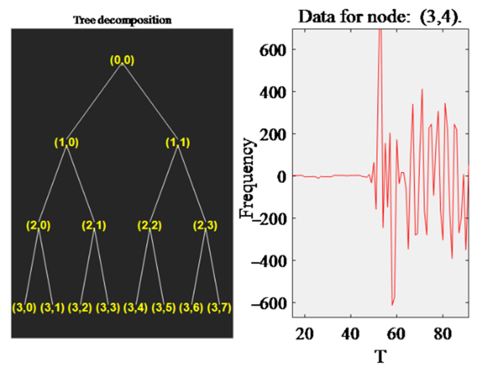
1.1.1. Wavelet Packet Decomposition

Wavelet packet decomposition is a signal analysis method that can improve the time domain resolution of signals and is more refined than wavelet decomposition. Wavelet packet decomposition is equivalent to a band-pass filter and a low-pass filter, at each time the original signal is decomposed into two sub-signals. The frequency between (0, 2π) is decomposed into (0, (2j − 1) π) and (2(j − 1) π, 2π), which are called approximation signal and detail signal, respectively. The next decomposition is for the frequency between (0, (2j − 1) π), and (2(j − 1) π, 2π), respectively. Wavelet packet decomposition is a multi-scale decomposition from top to bottom, and the adjacent signals in each scale are independent components. After the j-th layer wavelet packet decomposition, the signal x(t) can be written as:
x ( t ) = i = 1 2 j x j i ( t )
where x j i ( t ) represents the signal of the i-th frequency band decomposed by the j-th layer.
In the specific signal x(t), the frequency band energy Ex is as follows:
E x = x 2 ( t ) d t = i = 1 2 j i = 1 2 j x j i ( t ) x j i * ( t ) d t
According to the orthogonality of wavelet packets, Equation (2) can be transformed into:
E x = i = 1 2 j E j i
where E j i = [ x j i ( t ) ] 2 d t , E j i is a signal energy of the i-th frequency band, and the total energy of the signal is equal to the sum of the signal energy of each frequency band.

1.1.2. Determining the Optimal Number of Decomposition Layers

In the wavelet packet decomposition process, the selection of the optimal decomposition level has an important influence on the extraction of acceleration signal features. The selection of the optimal number of decomposition layers should not only cover the main damage information, but also not increase the amount of calculation. In this study, the wavelet packet energy entropy is used as the criterion for the selection of the optimal number of decomposition layers [28,29], which can represent the disorder degree of energy information. When the energy entropy value of the wavelet packet increases, the disorder of the information becomes higher, the contribution of useful energy information is smaller, and the calculation amount increases [30]. Therefore, the wavelet packet energy entropy function Es is selected as the loss function of the optimal number of decomposition layers, and its expression is as follows:
E s = - i = 1 i = 2 j p i lg p i
p i = E i i = 1 2 j E i
where Ei is the energy value of each frequency band, and pi represents the percentage of the energy of each frequency band in the total frequency band. j represents the number of decomposition layers, i represents the number of frequency bands, and the decomposition of each layer has 2 j frequency bands.
When determining the optimal number of decomposition layers, it is necessary to start the search from the top layer of the wavelet packet tree. If the loss function of a parent node is greater than the sum of the loss functions of its two child nodes, it means that the decomposition of this layer can decompose the original signal into more regular sub-signals, the energy is more concentrated, and the provided feature information contributes greatly. Conversely, if the sum of the loss functions of the two sub-nodes is greater than that of the parent node, it means that the signal is over-decomposed. Because the entropy value of the signal becomes larger after the decomposition (that is, the disorder degree of the signal becomes larger), the energy becomes scattered, which is not as great as the contribution of the feature information provided before the decomposition. We traversed all the node loss function values under the decomposition of each layer. When the sum of the loss function values is the smallest, the decomposition of this layer is the optimal number of decomposition layers.

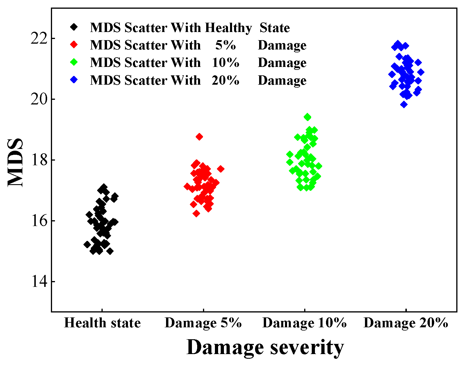
1.2. MDS (Square of Mahalanobis Distance)

Mahalanobis distance was proposed by Indian statisticians in 1936, and it is a common distance indicator in metric learning, which is used to evaluate the similarity between data. The multi-dimensional band energy extracted by wavelet packet decomposition cannot establish unified information, while the Mahalanobis distance can eliminate the interference of the correlation between variables, maintain the scale invariance, and correlation, which prove unaffected by the dimension. To construct an index that can reflect bridge damage information, this paper uses Mahalanobis distance to fuse multi-dimensional feature vectors.
Suppose Xp × q = [xij]p×q, i = 1, 2, …p, j = 1, 2, …q, Yp×q = [yij]p×q, i = 1, 2, …p, j = 1, 2, …q, represents the multi-dimensional feature vector sets of healthy samples and damaged samples under the same decomposition level, where xij represents the i-th healthy sample value of the j-th feature; p is the number of samples, q is the the number of eigenvectors, similar to the representation method under known damage samples. The most important step in the Mahalanobis distance method is to eliminate the dimensional relationship between the feature vectors and standardize X and Y. The specific process is as follows:
z i j = ( x i j y i j ) / σ j
σ j = i = 1 a ( x i j y i j ) 2 a 1
In the formula, a is the number of healthy sample data, Z is the data value of [X−Y] after normalization, assuming C is the covariance matrix of [X−Y] after normalization, and the covariance matrix C calculates the covariance between different dimensions instead of the covariance between samples. When constructing the covariance matrix, it should be noted that the number of samples is greater than the number of dimensions [31]. Then the square of the Mahalanobis distance of the feature vector set can be calculated by the following formula:
M D S ( i ) = z i j C 1 z i j

1.3. Simulated Annealing Particle Swarm Optimization (SAPSO)

1.3.1. Improvement Process of SAPSO Algorithm

Particle swarm optimization is a process simulating birds in a flock by designing a massless particle, and giving the particle velocity and position two attributes to search for the optimal solution separately in the search space at the same time [32,33]. Because the standard PSO is prone to premature convergence and it has been proven that the algorithm is not globally convergent [34], the search performance of standard PSO can be improved by combining the idea of simulated annealing, which can effectively prevent the search from falling into local extreme values. The addition of the idea of simulated annealing can control the performance whether the particles enter the next search area to search through the temperature, thereby enhancing the local search ability of the particles.
SAPSO is based on the standard PSO operation process, introducing the simulated annealing mechanism as a local search to further optimize and adjust the particles. First and foremost, the initial group is generated randomly. Then, random search is beginning, where new individuals are generated through the standard PSO. Finally, simulated annealing is performed on the generated local optimal individuals to determine whether the result can be used as the next generation group until the optimal optimization is achieved. The particle update mechanism of SAPSO before improvement is as follows:
p a r t V i j ( t + 1 ) = p a r t V i j ( t ) + c 1 × r a n d ( ) × ( p b e s t x i j ( t ) p a r t x i j ( t ) ) + c 2 × r a n d ( ) × ( g b e s t x i j ( t ) p a r t x i j ( t ) )
where partVi’ represents the current speed of the particle, pbestxi’ is the distance between the current position of a particle and its best position, partxi’ is the current position of a particle, gbestxi’ is the distance between the current position of a particle and the best position of the group, i’ represents the i’th particle, j’ represents the dimension of the actual problem, t is the number of iterations, and rand() is a random number uniformly distributed between 0 and 1.
There are three primary parts in the new speed of particle i’: (1) the speed of the particle at the previous moment; (2) the distance between the current position of the particle and its own best position; (3) the distance between the particle’s current position and the best position of the swarm.
According to Equation (9), the speed of the algorithm before the improvement is primarily updated by the speed of the particle at the previous moment and the current position. However, when the first item “partVi’” in the equation is 0, the new method is only related to the current position, and the algorithm is prone to falling into the local optimal solution. To improve the global search ability of the algorithm, different improvements are made in the study of particle swarm inertial weight, thus the inertial weight coefficient H is introduced as the proportional coefficient related to the speed at the previous moment. The setting of the inertia weight H has an important influence on the convergence speed and results of the algorithm [35]. A larger H has a stronger global search ability. Conversely, a smaller H is beneficial to local search. Therefore, the accurate adjustment of H can create the local search method first used in the process of search optimization in the actual problem. After a search fails to achieve the desired result, the full search is initiated to expand the scope and make the results more precise.
The speed updating after adding the inertia weight H becomes:
p a r t V i j ( t + 1 ) = H × p a r t V i j ( t ) + c 1 × r a n d ( ) × ( p b e s t x i j ( t ) p a r t x i j ( t ) ) + c 2 × r a n d ( ) × ( g b e s t x i j ( t ) p a r t x i j ( t ) )
The inertia weight is:
H = H min + ( H max H min ) × tanh ( i t e r )
where Hmax and Hmin are the maximum and minimum values of the inertia weight, respectively, and the general value range is: 0.4~0.95, iter represents the number of runs. The tanh(x) function’s features introduced is that when the area of the positive semi-axis of x, the value range is [0, 1] [36].
While the inertia weight coefficient is changed from small to large, the problem of local search and comprehensive search can be solved in the actual problem.

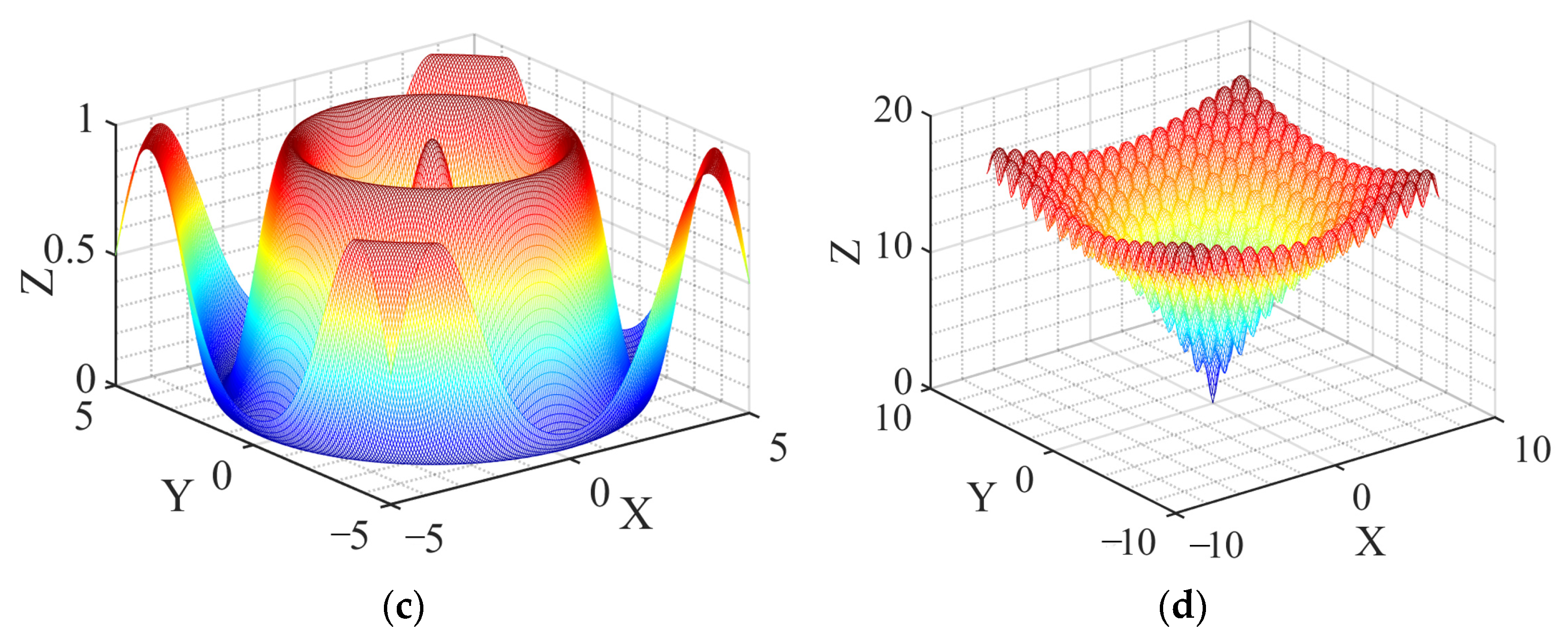
1.3.2. Improved Hyperbolic Tangent Function-Simulated Annealing Particle Swarm Optimization (HTF-SAPSO)

In order to evaluate the actual optimization performance of HTF-SAPSO, four common benchmark functions (Figure 1) are introduced for testing the performance of HTF-SAPSO, portrayed as follows:
f 1 ( x ) = i = 1 30 x i 2 , x i [ 100 , 100 ]
f 2 ( x ) = i = 1 30 [ x i 2 10 cos ( 2 π x i ) + 10 ] , x i [ 5 , 5 ]
f 3 ( x ) = 0.5 + ( ( sin ( x 1 2 + x 2 2 ) 0.5 ) 0.5 ) / ( 1 + 0.001 ( x 1 2 + x 2 2 ) ) 2 , x i [ 5 , 5 ]
f 4 ( x ) = 20 × e 0.2 × i = 1 80 x i 2 / 80 e i = 1 80 cos ( 2 π x i ) / 80 + 20 + e , x i [ 10 , 10 ]
To test the global convergence speed of the improved algorithm and the ability to jump out of local optimization, this characteristic tests function are specially used for testing, and the image of the above test function is provided, which is to help readers understand the optimization process of the algorithm. There is no correlation between the dimension of and the number of design parameters.
The iterative processes based on the four benchmark functions are portrayaed as in Figure 2.
According to the calculation results and iterative graphs of the above multi-dimensional complex benchmark functions, HTF-SAPSO has a certain improvement in calculation efficiency and calculation accuracy compared with SAPSO. Its convergence speed is faster and the global search ability is stronger, which can achieve a global optimization solution.
The identification process of damage severity based on HTF-SAPSO is as follows:
  • Set the population size N, particle dimension D, and initialize the speed and position of the particle;
  • Calculate the fitness value of each particle Fitness(x) [37], store the individual optimal value of each particle xG, and store the global optimal value of all particles xGbest;
  • Set the initial temperature T0;
  • Update the inertia weights according to Equations (10) and (11), and calculate the fitness value Fitness(x) for the updated particles;
  • The Metropolis mechanism of the simulated annealing algorithm is used to judge whether the particle can be used as a new optimal solution, and the global optimal solution is generated in the same way;
  • Perform the cooling operation Titer = 0.9 × Titer;
  • Determine whether the termination condition is met, and if so, output xGbest; otherwise, re-execute step 4.

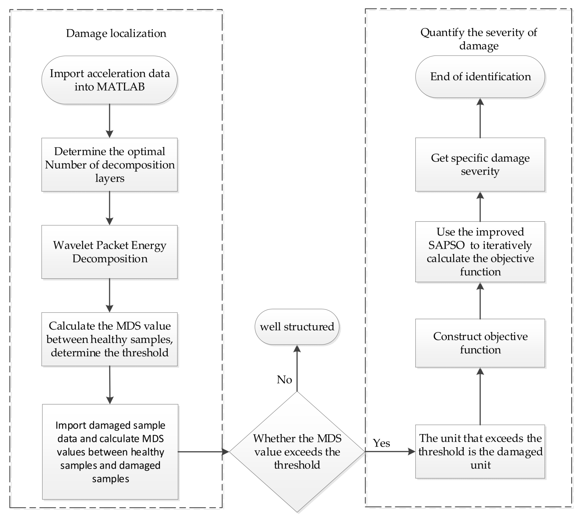
1.4. Damage Identification Method

1.4.1. Defining Damage Identification Vectors

The wavelet packet energy eigenvector of the structure’s dynamic response is not the inherent dynamic characteristic parameter of the structure, it is directly related to the load excitation of the structure. Although the load excitation is guaranteed to be regular, the wavelet packet energy eigenvector under non-stationary environment excitation still has certain volatility and randomness. Therefore, in this paper, the signal length is grouped, and the mean value of the calculated data is taken as the result. It is assumed that the length of the monitoring data sample is l which is divided into m groups equally, and the data length of each group is n, l = m × n [15,38]. The MDS between the k-th healthy samples can be calculated as follows:
M D S k = [ X - X * ] T S - 1 [ X - X * ]
Similarly, the MDS between the healthy samples and the damaged samples can be calculated according to Equation (13):
M D S k = ( X Y ) T S 1 ( X Y )
The damage identification vector Rtv between healthy samples is the vector formed by taking the average of the MDS values of each group, which is as follows:
R t v = k = 1 m [ X X * ] T S 1 [ X X * ] m 1
Similarly, the damage identification vector Rtu between the healthy sample and the damaged sample is a vector formed by taking the average of the MDS values of each group:
R t u = k = 1 m ( X Y ) T S 1 ( X Y ) m
Then the damage identification vector between healthy samples and damaged samples under the global element can be expressed as (Rt1, Rt2,…, Rtu)T, and the damage identification vector between healthy samples [X] to [X*] under the global element can be expressed as (Rt1, Rt2, …, Rtv)T, where [X] and [X*] represent the energy frequency bands under the same decomposition level in the adjacent two groups of healthy samples.

1.4.2. Building the Objective Function

Based on wavelet packet energy and the Mahalanobis distance squared (WPE-MDS), the objective function is constructed based on the change rate between the MDS value of the element that exceeds the MDS value in the healthy state and the MDS mean value in the healthy state:
F = | R t u × λ - M D T M D T | = | R t u × λ M D T 1 |
M D T = v = 1 w R t v / w + 1.05 ( 1 β ) 2 × C
where Rtu is the damage identification vector at the element u between the healthy sample and the damaged sample. Rtv is the damage identification vector at the element v between the healthy samples. w is the total number of nodes under the healthy sample. v = 1 w R t v / w is the mean of MDS values between healthy samples, and uses the probability threshold method to determine the MDT as the threshold [39,40], the β approximation is the proportion of the repeated data of Rtv in the healthy sample, and C is the standard deviation of the Rtv data in the healthy sample. λ = (λ1, …, λu) ∈ [0, 1], indicated as design variable, whose value is the damage severity of u elements. The unknown λ is the damage severity of the required structural element when the function F takes the minimum value.

1.4.3. Identification Steps

Using the improved HTF-SAPSO algorithm in this paper, Equation (14) is solved and optimized, and the damage severity of the structure is calculated. The basic process of the research method for damage identification based on WPE-MDS and HTF-SAPSO is portrayed in Figure 3. The main steps are as follows:
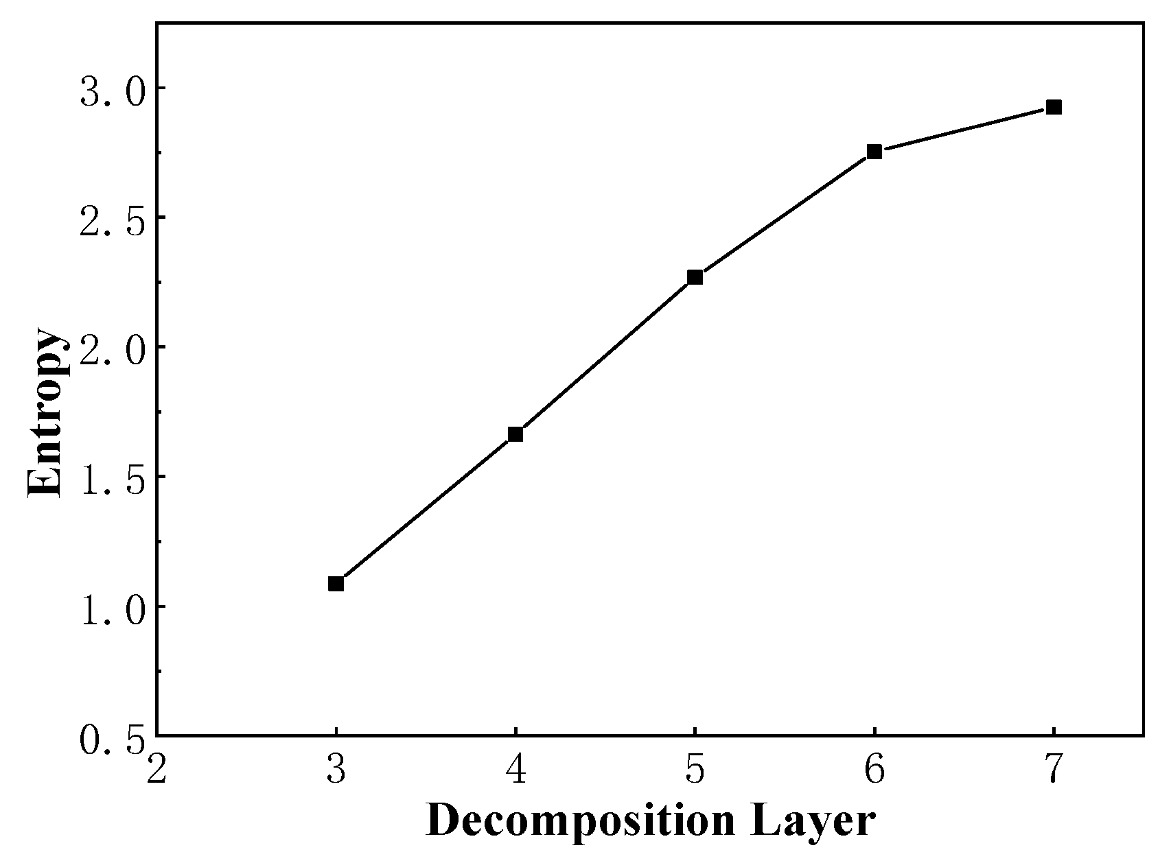
  • Determination of the optimal number of decomposition layers: the time-history response signal of the structure through Newmark is obtained, and 3–7 layers of wavelet packet energy decomposition for the groups of healthy samples and damaged samples with large changes in acceleration signals are performed. The energy entropy of the wavelet packet is calculated with the obtained energy value under decomposition, and then the optimal number of decomposition layers is determined.
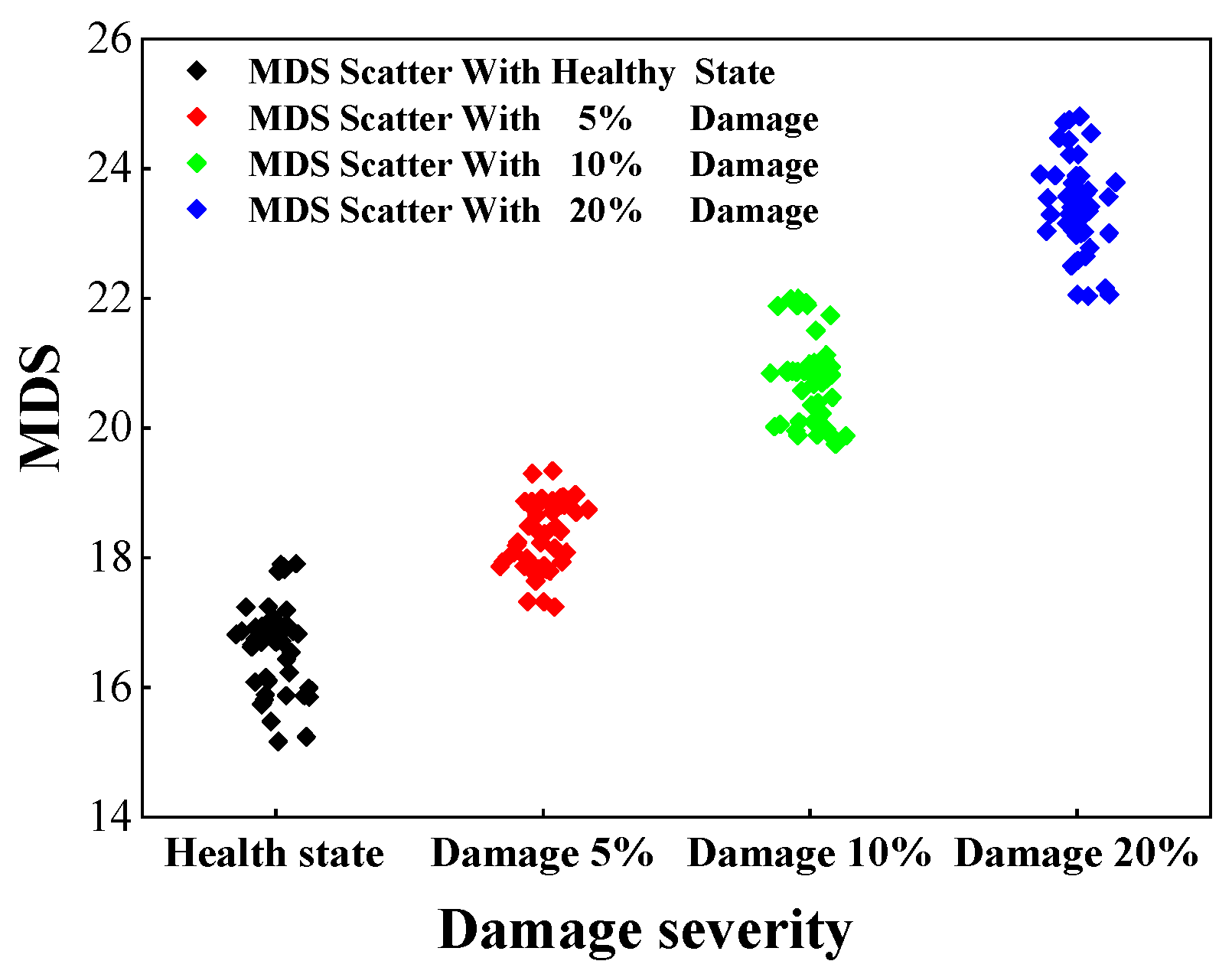
  • Calculation of the MDS value between healthy samples: wavelet packet energy decomposition is conducted to perform optimal decomposition layer decomposition on the healthy sample grouped data in step (1). In turn, the MDS values are calculated for the decomposed energy frequency bands [X] and [X*] of the adjacent two groups in healthy samples, and the node MDS values are averaged to obtain the threshold.
  • Calculation of the MDS value between the healthy sample and the damaged sample: the MDS value is calculated for each group of decomposed energy frequency band [X] under the healthy sample and the energy frequency band [Y] under the damaged sample in turn.
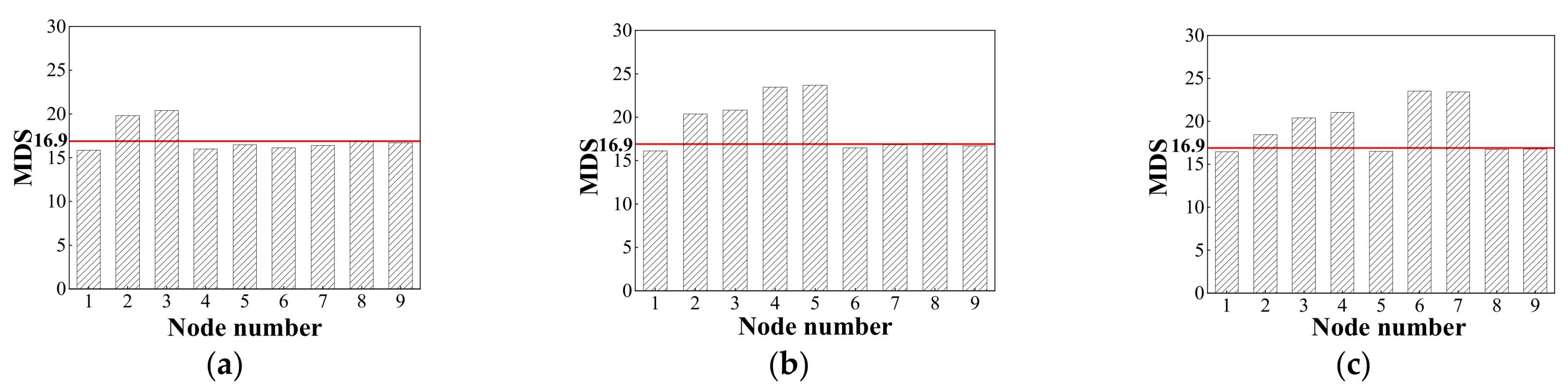
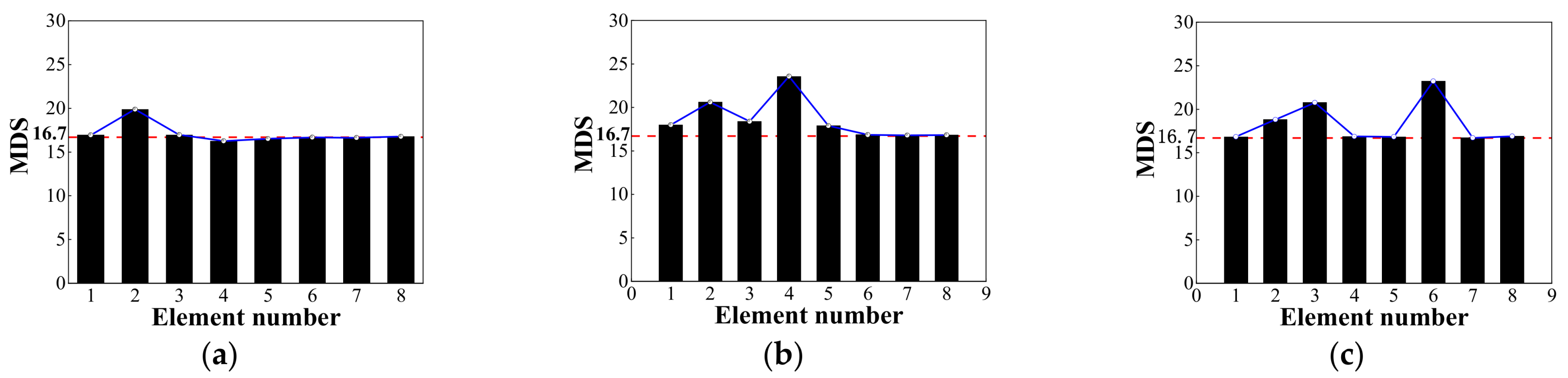
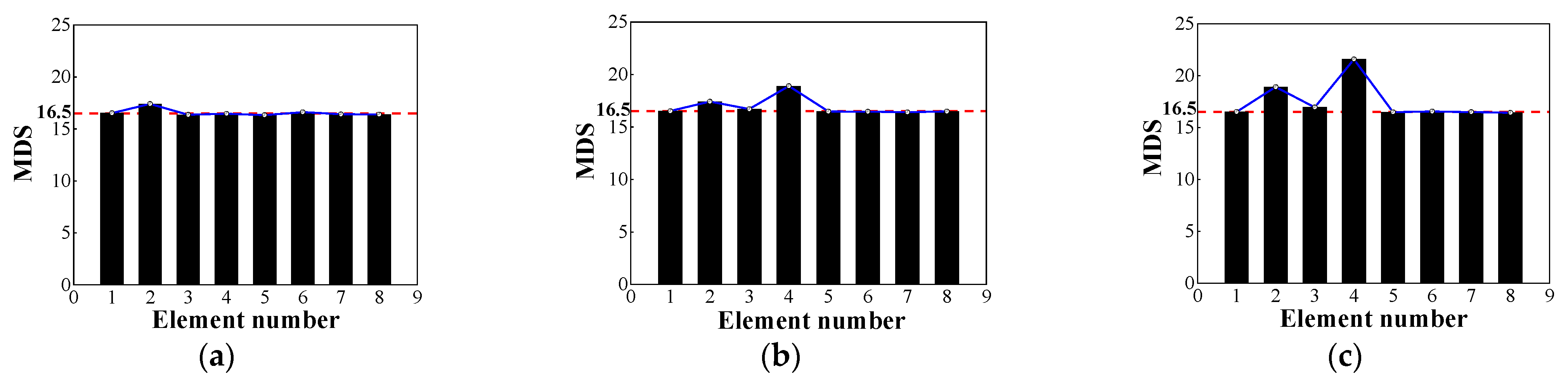
  • Damage location identification: The MDS values obtained by solving all the grouped data are averaged, and the damage location judgment is based on whether the MDS values under each node are higher than the threshold.
  • Damage severity identification: The damage severity is only identified for the damaged elements identified in step 4, and the HTF-SAPSO algorithm is used to optimize the objective function to identify the damage severity.

2. Numerical Simulation
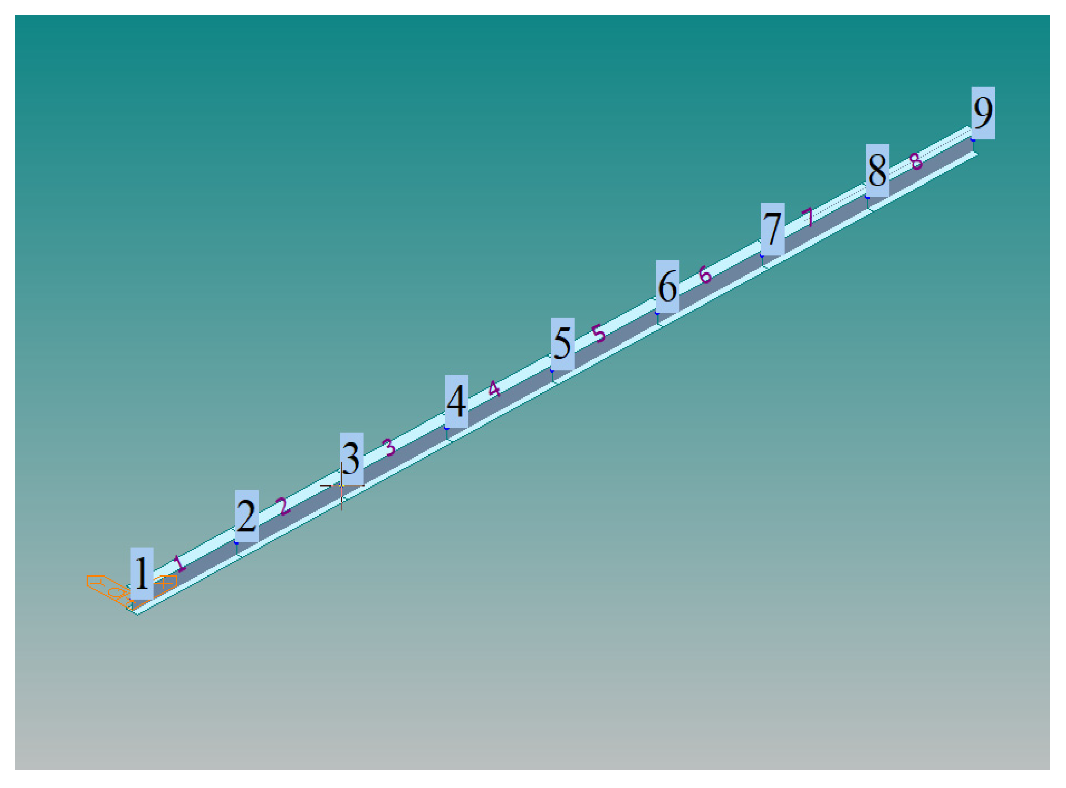
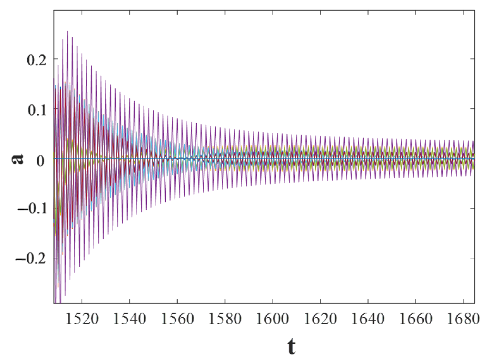
2.1. I-Beam Model

To preliminarily verify the feasibility of bridge damage location and damage severity identification based on the WPE-MDS method, this section establishes the I-beam for numerical simulation analysis and calculation, and establishes the finite element model of the I-beam, which is portrayed in Figure 4 and based on MATLAB platform. The beam has a total length of 5 m and is divided into 8 elements using 9 nodes, each of which is 0.625 m in length. The element used is a 2-Node 6-DOF element with an elastic modulus of 206 GPa, a cross-sectional area of 0.0014 m2, and a cross-sectional moment of inertia of 2.45 × 10⁻⁶ m4. We defined the element stiffness matrix and the element mass matrix and used them to assemble the global stiffness matrix and the global mass matrix. Finally, the dynamic response of the structure is calculated by the Newmark method.

2.2. Setting the Damage Case

In this excitation, the external load is simulated in the form of a concentrated load which is applied at the node #5, and where the action time is 15 s, the sampling frequency is 0.01 s, and the acceleration time history of each node in the whole process is recorded. The stiffness reduction method is utilized to simulate the structural damage, where three damage cases, single point damage, two-point damage, and multipoint damage are considered and set up. Considering that noise is a non-negligible influencing factor in practical engineering, noises with different levels are added for the three damage cases, as indicated in Table 1.
The noise of the numerical vibration response signal is assumed to be white noise conforming to the Gaussian distribution. White noise data is added to the acceleration signal of each measuring point according to Equation (15) [41]:
a u z = a u + a u max × r a n d n × n s
where au and a u z are the acceleration signals before and after adding noise at the u measurement point respectively, randn represents Gaussian white noise with a mean of 0 and a standard deviation of 1, and ns represents the noise level of the acceleration signal, which indicates that the standard deviation of the added noise is ns times the maximum acceleration of the measuring point.
Among them, ns is obtained by the signal-to-noise ratio SNR, and the equation for calculating the signal-to-noise ratio of the acceleration signal at the u measurement point is as follows:
S N R j = 10 × l g ( 1 T t = 1 T a u t 2 1 T t = 1 T d u t 2 )
where aut is the acceleration value of the measurement point u at time t, dut is the noise value of measurement point u at time t, and T is the total number of times. The corresponding relationship between ns and SNR is portrayed in Table 2.

2.3. Determine the Optimal Number of Decomposition Layers

The acceleration data of each node was extracted by the Newmark method and imported into MATLAB for analysis. The optimal wavelet packet decomposition layers adopt the data of node 2 under Case 1 as an example, as indicated in Figure 5. Figure 6 is the excerpted signal of the wavelet packet tree at the node and the corresponding (3, 4) node obtained after decomposing the wavelet packet.
Because the wavelet packet decomposition level is too low, it is easy to cause the wavelet packet energy characteristics of the structural response signal to be inconspicuous. Convsersely, if the decomposition level is too high, the useful information will be eliminated. In this study, the number of decomposition layers is set to be 3–7 layers. It can be observed from Figure 5 that the acceleration response of 2-node at 3 layers of decomposition has the lowest damage function entropy value when the number of decomposition layers is 3–7, which indicates that the characteristic contribution of the damage information contained is the highest. Concurrently, according to the sampling theorem [42,43], the maximum frequency of the signal is 400 Hz, so the 3-layer decomposition has met the accuracy requirements, and the optimal number of decomposition layers in this study is 3.

2.4. Damage Identification and Analysis

Figure 7 portrays the acceleration data of the two nodes, which is grouped according to n = 200, the MDS values of the elements with different damage severity are calculated, and 30 groups are selected to draw a scatter diagram, as indicated in Figure 8.
It can be observed from Figure 8 that with the increase of the damage severity, the MDS increases correspondingly. In the healthy state, the MDS values are distributed in the interval of 16–18, and the threshold is 16.9. The MDS values with the preset damage severity of 5%, 10%, 20% are 17.8–19.1, 19.3–22 and 22–24.8, respectively.
By extracting the acceleration data at each node for processing, the MDS values at the node may be obtained. The node MDS average value under the healthy sample is selected as the threshold for identifying the damage location, which is used to judge whether the structure is damaged or not. When the node MDS value is above the threshold, it means that the structure is damaged. Conversely, it means that the structure is not damaged.
It can be clearly observed from Figure 9 that the maximum value of nodes 2, 3 under Case 1, nodes 2, 3, 4, and 5 under Case 2 and nodes 2, 3, 4, 6, and 7 under Case 3 are above the threshold line in bar charts. However, it is necessary to use the MDS information of the two nodes attached to the element at the same time when judging whether the element is damaged or not, according to the abnormal value of the node MDS. When the MDS value of only one node is abnormal, it is difficult to determine which element the corrupted node information belongs to, so the following research uses the element center acceleration signal to perform damage identification research.

2.4.1. Damage Localization Results

Based on the acceleration data through the center of the element, the bar graphs of element MDS values for Cases 1, 2, and 3 are portrayed in Figure 10.
It can be seen from Figure 10 that the tops of the element MDS bar graphs are connected successively, and the position of the broken line protrusion can be more clearly seen, where the abscissa corresponding to the protrusion position represents the code of the damaged element. There are obvious protrudes at element #2 in Case 1, elements #2 and #4 in Case 2, and elements #2, #3, and #6 in Case 3, which corresponds to the damage of the preset elements. The MDS values of elements #1, #3, and #5 in Case 2 are all above the threshold line of 16.5, and a small amount of damage occurs, which may be because it is close to the damaged element [11,15]. The error is within the acceptable range, which proves that the location of structural damage can be accurately judged by the abnormal MDS value of the element. Figure 9 and Figure 10 indicate the effect of damage localization, which indicates that it is more obvious to select the acceleration data at the center of two nodes for analysis than that at the nodes. Therefore, the damage location of the element can be more accurately identified by selecting the acceleration data at the center of the two nodes for processing.

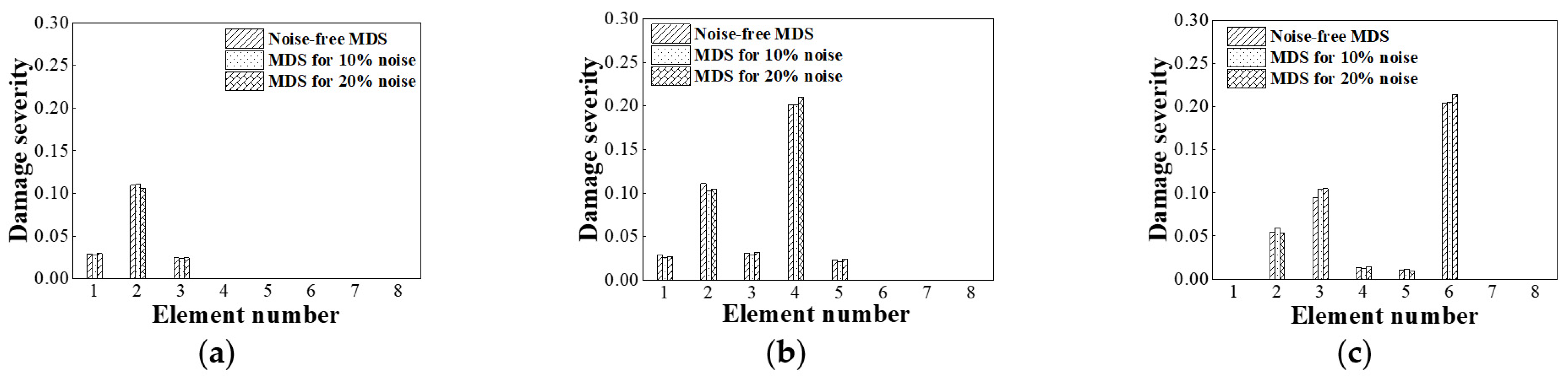
2.4.2. Damage Severity Identification Results

After the damage localization, the damage severity of the structure is quantitatively identified, and the damage severity results of each case are portrayed in Figure 11.
It can be observed from Figure 11 that the damage severity calculated under the three cases is mostly consistent with the preset damage severity of each element. There are some elements identified as damaged around the main damaged element, which may be due to the short distance from them to the primary damaged element [11,15], but the damage severity of the adjacent damaged elements is within the allowable error range. Therefore, the change rate between the MDS value of the element that exceeds the MDS value in the healthy state and the MDS mean value in the healthy state is defined as the objective function, and the improved HTF-SAPSO algorithm is used for iterative operation to quantify the damage severity, where the research method has a good identification effect. In summary, it can be preliminarily verified that the research method for structural damage identification based on WPE-MDS and HTF-SAPSO is feasible.

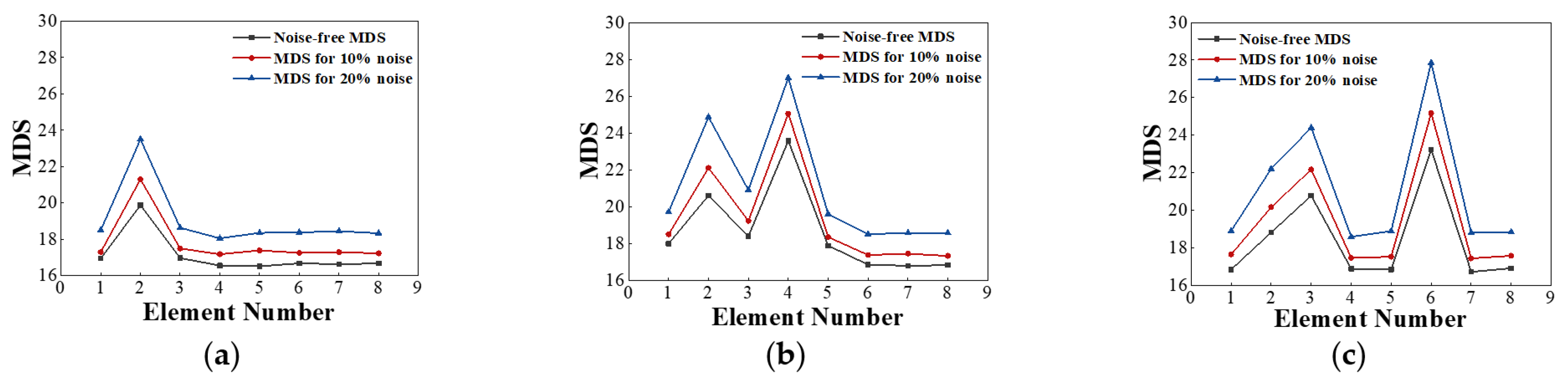
2.5. Damage Identification Considering the Influence of Noise

To simulate the real environment for the numerical model, different levels of noise are added under each damage case to investigate the change of the MDS value. According to Equation (17), white noise is added to the acceleration data, and the damage identification results are portrayed in Figure 12.
Figure 12a–c above indicate the changes in MDS values after adding different levels of noise in Cases 1, 2, and 3. In the noise-added environment, the MDS value of the element in the healthy state and the MDS value of the damaged element are both increased. With the increase of the noise-added level, the increase of the MDS value also accelerated. For example, in the process from no noise to 10% noise, the MDS value of element 7 increases by 4% in Case 3, while in the process from adding 10% noise to 20% noise, the MDS value increases by 6%. At the primary damaged element location, the rate of increase is greater than that at the healthy state node. For example, the MDS value of element #2 changes from 20.6 to 22.5 and then to 24.8 in Case 2, while the MDS value of element #3 in the healthy state changes from 18.4 to 19.6 at 10% noise and then to 20.9 at 20% noise.
The effect of adding different levels of noise on the damage severity results of each case is portrayed in Figure 13.
In accordance with the increase of the noise addition ratio, it can be observed from Figure 13 that the damage identification results of damaged elements under each case are essentially unchanged and remain constant. The results indicate that the method proposed in this paper is of good robustness.

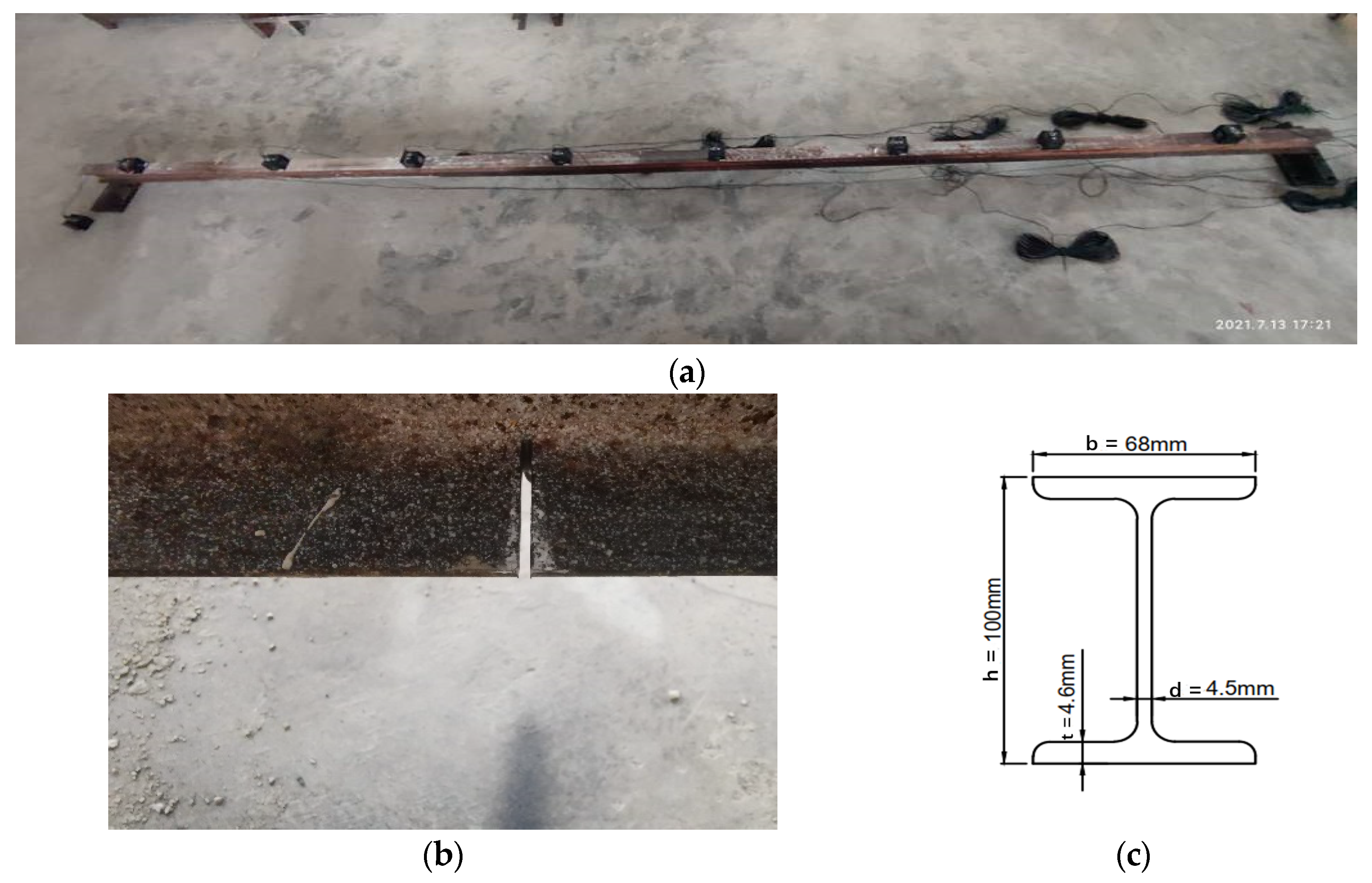
3. Experimental Test

3.1. Introduction to the Test

An I-shaped steel beam (Figure 14) was used for the research, which is with a length of 5 m, a cross-sectional area of 0.0014 m2, a Young’s modulus of 2.0 × 10¹¹ Pa, and a mass density of 7850 kg/m3. The full length is divided into 8 elements with 9 nodes, the length of each element is 0.625 m, and the 8 sensors are placed in the center of the 8 elements, respectively.

3.2. Setting the Damage Case

Damage in this experiment is adopted by cutting an I-beam with a different depth, and the stiffness reduction is calculated according to Equation (19). The test is set up with a group of non-destructive cases and 3 damaged cases (Table 3). The settings of each case in the entire test are as follows:
β = p × q p e × q e
where pe and p are the lengths of the intact and cut elements respectively, qe and q are the widths of the intact and cut elements, respectively.

3.3. Damage Identification Analysis

The measured acceleration data is displayed in Figure 15. After integrating the MDS values of different damage severities in each case, it is discovered that the MDS values of the same damage severity in different cases are close, and the results are indicated in Figure 16.
As can be observed from Figure 16, the element MDS values of healthy state, 5%, 10%, and 20% damaged elements are concentrated in the range of 15–17, 16–18, 17–19, and 20–22, respectively. The damage localization results and damage quantification results are demonstrated in Figure 17 and Figure 18, respectively.
In Figure 17, the top of the bar graph is connected successively. The protruding part of the broken line corresponds to the element number of the damaged location under each case. There are abnormal MDS values for element #2 in Case 1, elements #2 and #4 in Case 2, and elements #2 and #4 in Case 3, and there are different degrees of protrusions on the connection lines at the corresponding elements, which is highly consistent with the damaged cut site. So, the research method based on WPE-MDS is feasible and can better identify the damage location.
It can be observed from Figure 18 that the primary damaged element under Case 1 is element #2, and the damage severity is 5%, which is consistent with the actual cutting damage. For Case 2, the damage of elements #2 and #4 is much higher than that of other elements, and the damage severity corresponds to 5% and 10% of the stiffness reduction. The damage of elements #2 and #4 under Case 3 is also higher than that of other elements, and the damage severity is consistent with the 10% and 20% of the stiffness reduction. Because the measured acceleration data is close to the cutting damage element, there will be small fluctuations [11,15]. Under the three cases, small damage is identified near the main damaged element, but it does not affect the damage severity of the main damaged element. Therefore, the damage severity can be better quantified based on the HTF-SAPSO algorithm.

4. Conclusions

In this paper, a research method based on the combination of WPE-MDS values and HTF-SAPSO algorithm is proposed to identify the severity of structural damage. First, the wavelet packet three-layer decomposition is performed based on the original monitored acceleration signal, and the MDS value between samples is calculated based on the frequency band energy value that obtained by the decomposition, where the damage location can be well identified according to the abnormal MDS value of the element. The change rate between the MDS value of the unit that exceeds the MDS value in the healthy state and the MDS mean value in the healthy state is defined as the objective function, and the improved HTF-SAPSO algorithm is used for iterative operation to quantify the damage severity. The feasibility and effectiveness of the method are verified by numerical simulations and experimental examples, respectively, and the primary conclusions are as follows:
(1)
The abnormal MDS value of the element obtained by the calculation based on the WPE-MDS value can be used to locate the damage, and then the HTF-SAPSO algorithm is used for the damage quantification method, which has a good damage identification effect. Among them, the performance of damage identification using the acceleration data of element midpoint and node is compared and analyzed, where the damage identification performance obtained by the former is better.
(2)
The addition of different noise ratios has different effects on the MDS value. As the noise ratio increases, the MDS value of node element also increases, which has a good amplification effect on damage location. The impact of same ratio noise on the MDS values of damaged elements and healthy elements is also different, and the result is that the damaged elements have a greater impact. According to the analysis results of the damage severity, the size of the noise ratio does not affect the damage severity, by which it can be proven that the method research based on WPE-MDS and HTF-SAPSO has strong robust performance;
(3)
Considering the particularity of the damaged signal as a time series, the HTF-SAPSO algorithm converges earlier than the SAPSO algorithm in the iterative operation of the objective function, which can improve the computational efficiency.

Author Contributions

Conceptualization, H.W.; data curation, H.W.; formal analysis, M.H. and H.W.; methodology, M.H. and H.W.; resources, M.H.; software, H.W. and Z.W.; writing—original draft, H.W.; writing—review and editing, M.H., Z.W. and Z.X. All authors have read and agreed to the published version of the manuscript.

Funding

This work was supported by the Graduate Innovative Fund of Wuhan Institute of Technology (No: CX2021128).

Institutional Review Board Statement

No applicable.

Informed Consent Statement

No applicable.

Data Availability Statement

Some or all data that support the findings of this study are available from the corresponding author upon reasonable request.

Conflicts of Interest

The authors declare that they have no conflict of interest.

References

  1. Hou, R.R.; Xia, Y. Review on the new development of vibration-based damage identification for civil engineering structures: 2010–2019. J. Sound Vib. 2021, 491, 115741. [Google Scholar] [CrossRef]
  2. Bagheri, A.; Zare, H.A.; Rizzo, P. Time domain damage localization and quantification in seismically excited structures using a limited number of sensors. J. Vib. Control 2017, 23, 2942–2961. [Google Scholar] [CrossRef]
  3. Obrien, E.J.; Malekjafarian, A.; González, A. Application of empirical mode decomposition to drive-by bridge damage detection. Eur. J. Mech. A/Solids 2017, 61, 151–163. [Google Scholar] [CrossRef] [Green Version]
  4. Razavi, M.; Hadidi, A. Structural damage identification through sensitivity-based finite element model updating and wavelet packet transform component energy. In Structures; Elsevier: Amsterdam, The Netherlands, 2021; Volume 33, pp. 4857–4870. [Google Scholar]
  5. Diao, Y.; Jia, D.; Liu, G. Structural damage identification using modified Hilbert-Huang transform and support vector machine. J. Civ. Struct. Health Monit. 2021, 11, 1155–1174. [Google Scholar] [CrossRef]
  6. Sony, S.; Sadhu, A. Multivariate empirical mode decomposition-based structural damage localization using limited sensors. J. Vib. Control 2022, 28, 2155–2167. [Google Scholar] [CrossRef] [PubMed]
  7. Liu, Y.Y.; Ju, Y.F.; Duan, C.D. Structure damage diagnosis using neural network and feature fusion. Eng. Appl. Artif. Intell. 2011, 24, 87–92. [Google Scholar] [CrossRef]
  8. Chen, Y.J.; Xie, S.L.; Zhang, X. Damage identification based on wavelet packet analysis method. Int. J. Appl. Electromagn. Mech. 2016, 52, 407–414. [Google Scholar] [CrossRef]
  9. Law, S.S.; Zhu, X.Q.; Tian, Y.J. Statistical damage classification method based on wavelet packet analysis. Struct. Eng. Mech. 2013, 46, 459–486. [Google Scholar] [CrossRef]
  10. Yeager, M.; Gregory, B.; Key, C. On using robust Mahalanobis distance estimations for feature discrimination in a damage detection scenario. Struct. Health Monit. 2019, 18, 245–253. [Google Scholar] [CrossRef]
  11. Mosavi, A.A.; Dickey, D.; Seracino, R. Identifying damage locations under ambient vibrations utilizing vector autoregressive models and Mahalanobis distances. Mech. Syst. Signal Process. 2012, 26, 254–267. [Google Scholar] [CrossRef]
  12. Deraemaeker, A.; Worden, K. A Comparison of linear approaches to filter out environmental effects in structural health monitoring. Mech. Syst. Signal Process. 2018, 105, 1–15. [Google Scholar] [CrossRef]
  13. Nguyen, T.; Chan, T.H.T.; Thambiratnam, D.P. Field validation of controlled Monte Carlo data generation for statistical damage identification employing Mahalanobis squared distance. Struct. Health Monit. 2014, 13, 473–488. [Google Scholar] [CrossRef] [Green Version]
  14. Tao, X.C.; Lu, C.; Lu, C.; Wang, Z.L. An approach to performance assessment and fault diagnosis for rotating machinery equipment. EURASIP J. Adv. Signal Process. 2013, 2013, 5. [Google Scholar] [CrossRef] [Green Version]
  15. Chen, C.; Wang, Y.H.; Wang, T. A Mahalanobis Distance Cumulant-Based Structural Damage Identification Method with IMFs and Fitting Residual of SHM Measurements. Math. Probl. Eng. 2020, 2020, 6932463. [Google Scholar] [CrossRef]
  16. Gres, S.; Ulriksen, M.D.; Döhler, M. Statistical methods for damage detection applied to civil structures. Procedia Eng. 2017, 199, 1919–1924. [Google Scholar] [CrossRef]
  17. Mohammadi Ghazi, R.; Büyüköztürk, O. Damage detection with small data set using energy-based nonlinear features. Struct. Control Health Monit. 2016, 23, 333–348. [Google Scholar] [CrossRef] [Green Version]
  18. Huang, M.S.; Li, X.F.; Lei, Y.Z. Structural damage identification based on modal frequency strain energy assurance criterion and flexibility using enhanced Moth-Flame optimization. Structures 2020, 28, 1119–1136. [Google Scholar] [CrossRef]
  19. Huang, M.S.; Cheng, X.H.; Lei, Y.Z. Structural damage identification based on substructure method and improved whale optimization algorithm. J. Civ. Struct. Health Monit. 2021, 11, 351–380. [Google Scholar] [CrossRef]
  20. Huang, M.S.; Lei, Y.Z.; Li, X.F. Structural damage identification based on l1regularization and bare bones particle swarm optimization with double jump strategy. Math. Probl. Eng. 2019, 2019, 5954104. [Google Scholar] [CrossRef] [Green Version]
  21. Huang, M.S.; Zhao, W.; Gu, J.F. Damage identification of a steel frame based on integration of time series and neural network under varying temperatures. Adv. Civ. Eng. 2020, 2020, 4284381. [Google Scholar] [CrossRef]
  22. Huang, M.S.; Lei, Y.Z.; Li, X.F. Damage identification of bridge structures considering temperature variations-based SVM and MFO. J. Aerosp. Eng. 2021, 34, 04020113. [Google Scholar] [CrossRef]
  23. Huang, M.S.; Cheng, X.H.; Zhu, Z.G. A novel two-stage structural damage identification method based on superposition of modal flexibility curvature and whale optimization algorithm. Int. J. Struct. Stab. Dyn. 2021, 21, 2150169. [Google Scholar] [CrossRef]
  24. Ravanfar, S.A.; Razak, H.A.; Ismail, Z. A two-step damage identification approach for beam structures based on wavelet transform and genetic algorithm. Meccanica 2016, 51, 635–653. [Google Scholar] [CrossRef]
  25. Katunin, A.; Przystałka, P. Damage assessment in composite plates using fractional wavelet transform of modal shapes with optimized selection of spatial wavelets. Eng. Appl. Artif. Intell. 2014, 30, 73–85. [Google Scholar] [CrossRef]
  26. Rosso, M.M.; Cucuzza, R.; Di Trapani, F. Nonpenalty machine learning constraint handling using PSO-SVM for structural optimization. Adv. Civ. Eng. 2021, 2021, 6617750. [Google Scholar] [CrossRef]
  27. Rosso, M.M.; Cucuzza, R.; Aloisio, A. Enhanced Multi-Strategy Particle Swarm Optimization for Constrained Problems with an Evolutionary-Strategies-Based Unfeasible Local Search Operator. Appl. Sci. 2022, 12, 2285. [Google Scholar] [CrossRef]
  28. Ekici, S.; Yildirim, S.; Poyraz, M. Energy and entropy-based feature extraction for locating fault on transmission lines by using neural network and wavelet packet decomposition. Expert Syst. Appl. 2008, 34, 2937–2944. [Google Scholar] [CrossRef]
  29. Zhang, L.; Xiong, G.; Liu, H. Fault diagnosis based on optimized node entropy using lifting wavelet packet transform and genetic algorithms. Proc. Inst. Mech. Eng. Part I J. Syst. Control Eng. 2010, 224, 557–573. [Google Scholar] [CrossRef]
  30. Etemad, K.; Chellappa, R. Separability-based multiscale basis selection and feature extraction for signal and image classification. IEEE Trans. Image Process. 1998, 7, 1453–1465. [Google Scholar] [CrossRef]
  31. Bulut, H. Mahalanobis distance based on minimum regularized covariance determinant estimators for high dimensional data. Commun. Stat. Theory Methods 2020, 49, 5897–5907. [Google Scholar] [CrossRef]
  32. Zhang, Y.; Wang, S.; Ji, G. A comprehensive survey on particle swarm optimization algorithm and its applications. Math. Probl. Eng. 2015, 2015, 931256. [Google Scholar] [CrossRef] [Green Version]
  33. Wang, L.; Liu, Y.Q. Application of simulated annealing particle swarm optimization based on correlation in parameter identification of induction motor. Math. Probl. Eng. 2018, 2018, 1869232. [Google Scholar] [CrossRef]
  34. Zhan, Z.; Zhang, J. Adaptive particle swarm optimization. In International Conference on Ant Colony Optimization and Swarm Intelligence; Springer: Berlin/Heidelberg, Germany, 2008; pp. 227–234. [Google Scholar]
  35. Shieh, H.L.; Kuo, C.C.; Chiang, C.M. Modified particle swarm optimization algorithm with simulated annealing behavior and its numerical verification. Appl. Math. Comput. 2011, 218, 4365–4383. [Google Scholar] [CrossRef]
  36. Guan, S.H.; Cheng, Q.; Zhao, Y. Robust adaptive filtering algorithms based on (inverse) hyperbolic sine function. PLoS ONE 2021, 16, e0258155. [Google Scholar] [CrossRef]
  37. Li, L.; Liang, Y.C.; Li, T. Boost particle swarm optimization with fitness estimation. Nat. Comput. 2019, 18, 229–247. [Google Scholar] [CrossRef]
  38. Aloisio, A.; Di Battista, L.; Alaggio, R. Sensitivity analysis of subspace-based damage indicators under changes in ambient excitation covariance, severity and location of damage. Eng. Struct. 2020, 208, 110235. [Google Scholar] [CrossRef]
  39. Ramlie, F.; Muhamad, W.Z.A.W.; Harudin, N. Classification performance of thresholding methods in the Mahalanobis-Taguchi system. Appl. Sci. 2021, 11, 3906. [Google Scholar] [CrossRef]
  40. Uchikawa, K.; Hoshino, T.; Nagai, T. Statistical significance testing with Mahalanobis distance for thresholds estimated from constant stimuli method. See. Perceiving 2011, 24, 91–124. [Google Scholar] [CrossRef] [Green Version]
  41. Seyedpoor, S.M.; Ahmadi, A.; Pahnabi, N. Structural damage detection using time domain responses and an optimization method. Inverse Probl. Sci. Eng. 2019, 27, 669–688. [Google Scholar] [CrossRef]
  42. Sasane, A. An abstract Nyquist criterion containing old and new results. arXiv 2010, arXiv:1002.4795. [Google Scholar] [CrossRef] [Green Version]
  43. Wang, Z.P.; Huang, M.S.; Gu, J.F. Temperature effects on vibration-based damage detection of a reinforced concrete slab. Appl. Sci. 2020, 10, 2869. [Google Scholar] [CrossRef] [Green Version]
Figure 1. Benchmark functions. (a) f 1 (x); (b) f 2 (x); (c) f 3 (x); (d) f 4 (x).
Buildings 12 01089 g001aBuildings 12 01089 g001b
Figure 2. Iteration Process of benchmark Functions. (a) f 1 (x); (b) f 2 (x); (c) f 3 (x); (d) f 4 (x).
Buildings 12 01089 g002
Figure 3. The step of identification process.
Buildings 12 01089 g003
Figure 4. Finite element model of the I-beam.
Buildings 12 01089 g004
Figure 5. The analysis of #2node decomposition level and entropy.
Buildings 12 01089 g005
Figure 6. The structure of 3-layer wavelet packet decomposition (left) and the signal of (3, 4) node (right).
Buildings 12 01089 g006
Figure 7. The acceleration time history graph of the case two.
Buildings 12 01089 g007
Figure 8. The scatter plot of MDS with different damage severities.
Buildings 12 01089 g008
Figure 9. Bar graph of MDS values for each damage case. (a) Case 1; (b) Case 2; (c) Case 3.
Buildings 12 01089 g009
Figure 10. Damage localization results. (a) Case 1; (b) Case 2; (c) Case 3.
Buildings 12 01089 g010
Figure 11. Identification results of damage severity. (a) Case 1; (b) Case 2; (c) Case 3.
Buildings 12 01089 g011
Figure 12. Changes in MDS before and after adding noise. (a) Case 1; (b) Case 2; (c) Case 3.
Buildings 12 01089 g012
Figure 13. Changes in damage severity before and after adding noise. (a) Case 1; (b) Case 2; (c) Case 3.
Buildings 12 01089 g013
Figure 14. The I-shaped steel beam. (a) sensor layout. (b) View of introduced damage. (c) Cross section.
Buildings 12 01089 g014
Figure 15. Acceleration time-history curve corresponding to Case 1.
Buildings 12 01089 g015
Figure 16. Scatter diagram of MDS values for each damage severity.
Buildings 12 01089 g016
Figure 17. Damage localization result map. (a) Description of Case 1; (b) Description of Case 2; (c) Description of Case 3.
Buildings 12 01089 g017
Figure 18. Identification result graph of damage severity. (a) Description of Case 1; (b) Description of Case 2; (c) Description of Case 3.
Buildings 12 01089 g018
Table 1. Damage cases of I-beam.
Damage CaseDamaged ElementSeverity of DamageNoise Level
1#210%0%, 10%, 20%
2#2, #410%, 20%0%, 10%, 20%
3#2, #3, #65%, 10%, 20%0%, 10%, 20%
Table 2. The relationship between ns and SNR.
SNR/dB806040201050
ns2.81 × 10−52.77 × 10−42.81 × 10−32.77 × 10−20.08780.1560.277
Table 3. Damage cases of the I-beam.
Damage CasePreset Damage SeverityDamaged Element
Healthy//
15%#2
25%, 10%#2, #4
310%, 20%#2, #4
Publisher’s Note: MDPI stays neutral with regard to jurisdictional claims in published maps and institutional affiliations.

