A New Method for Design of the Semi-Rigid Steel Frame—The Integration of Joint Inverse Design and Structural Design

Abstract

In the past few decades, semi-rigid connections have been studied extensively; several major international steel structure design specifications have incorporated this component into their own systems. However, there is still no appropriate way to integrate the semi-rigid joint design into the structural design more efficiently. The forward design method of introducing joint characteristics into the frame by predetermining joint details requires considerable effort to trial massive amounts of variables, which is undoubtedly a nightmare for those structures composed of thousands of members and joints. In this paper, a feasible method for the reversed design of semi-rigid steel frames has been developed. Being similar to the traditional one, the structural design is still divided into member design and joint design. In the member design phase, a joint is abstracted as a performance parameter and its details are no longer concerned. Then, in the joint design phase, the joint details can be reconstructed subject to the joint required performance by using the optimization algorithm. Throughout the process, engineers simply tune the desired properties of the joins rather than their construction geometry, which results in clearer tuning direction and improved solution efficiency. In addition, determining how to choose a good, required connection stiffness as the starting design is discussed and recommendations are given. Finally, two examples are solved to verify the effectiveness of the proposed method.

1. Introduction

The rotational stiffness of the beam-to-column joint plays an important role in steel structures since it directly affects the deformation, internal forces distribution, and stability of the structure [1]. Although the assumption of pinned or rigid joints simplifies the structural model and is more convenient for designers’ daily work, most of the joints used in practice have a certain rotational stiffness, which is called semi-rigid joints. The potential risks posed by this discrepancy between reality and assumptions are inaccuracy and insecurity in structural design [2,3]. Moreover, this problem is becoming more prominent with the bolted connections that are used extensively in modern steel structures, since many research results [4,5,6,7] have confirmed that the use of these types of semi-rigid joints can effectively reduce the cost of joint manufacturing and field erection and is a more economical scheme. At present, the provisions for structural steel buildings in various countries [8,9,10] clearly indicate that the real behavior of the joint should be considered. The moment–rotation curve of the joint should be assumed during the structure analysis, and the properties of the final joint must be guaranteed to conform to the pre-assumption.

Before proceeding with the design of semi-rigid steel frames, two key issues need to be addressed. One is how to establish a joint model; the other is how to integrate the semi-rigid joint design with the member design in a convenient way.

For the former, research has been conducted and various joint models and databases have been proposed. From elastic, to inelastic ultimate, to post-ultimate and post-fracture ranges [11,12,13,14]. From open-section joints, to closed-section joints, pure steel structural joints to composite structural joints [15,16,17]. From standard static loading to fire and seismic loading, 2D in-plane loading, to 3D space loading [18,19,20,21]. Diaz [22] summarized the existing computational models and pointed out that the Component Method (CM) attracts the most attention and has been developed mostly due to its clear physical meaning and low computational cost. This method can be applied to almost any type of joint, provided that the effective mechanical components in the joint are reasonably decomposed. EN1993-1-8 [23] is the first standard in the world to incorporate CM into structural design, which combined with SCI P398 [24] to provide extensive guidelines for calculating the strength, stiffness, and rotational capacity of joints. However, decomposing and assembling the joint components is a rather time-consuming and complex task, which limits the exploitation of advanced possibilities for engineers. In this context, Jaspart [25], Weynand, and Feldman [26] proposed some useful tools based on EN1993-1-8, including design tables, sheets, and software. Furthermore, the introduction of commercial software [27,28] has made the design of semi-rigid joints very easy, with quick results in just a few clicks.

In contrast, limited open literature to date has reported the latter, although attempts to this aspect had been made in the early stages of the research of semi-rigid joints. Xu et al. [29] firstly used the modified semi-rigid beam element for structural analysis. In their study, the joint stiffness was only defined as a real number within a certain range without involving any joint configuration parameters. Subsequently, Dhillon and O’Malley [30] developed an interactive design method for semi-rigid steel frames. By using the Fry–Morris model [31] to define the joint moment–rotation curve, engineers can interact with the computer to change the connection details and obtain an economical and practical design. To overcome the difficulty of estimating the joint stiffness in the preliminary frame design phase in which the joints have not been designed yet. Steenhuis et al. [6,32] introduced the conception of joint pre-design into the traditional steel structure design process. In a similar way, Bayo et al. [33] relaxed the assumption of joint pre-design to some extent by introducing more variables that affect the joint properties and proposed a practical method that can simultaneously optimize the member profile size and the joint details.

In general, all of the above design methods of semi-rigid steel frames are essentially a kind of forward method. That is, the initial rotational stiffness of the joint is calculated by more or less pre-set joint geometric parameters, and then introduced into the structural model for analysis and member design, finally, the joint details need to be refined to ensure that the obtained joint properties meet the previous assumptions. However, in the design practice, the joint configuration parameters are diverse and complex, as well as sensitive to the joint properties. It is difficult for engineers who do not have an in-depth knowledge of semi-rigid joints to grasp the direction of adjustment when designing. Despite the many advantages of semi-rigid steel frames, their practical application is rare due to the lack of proper design methods. Therefore, developing convenient methods is essential.

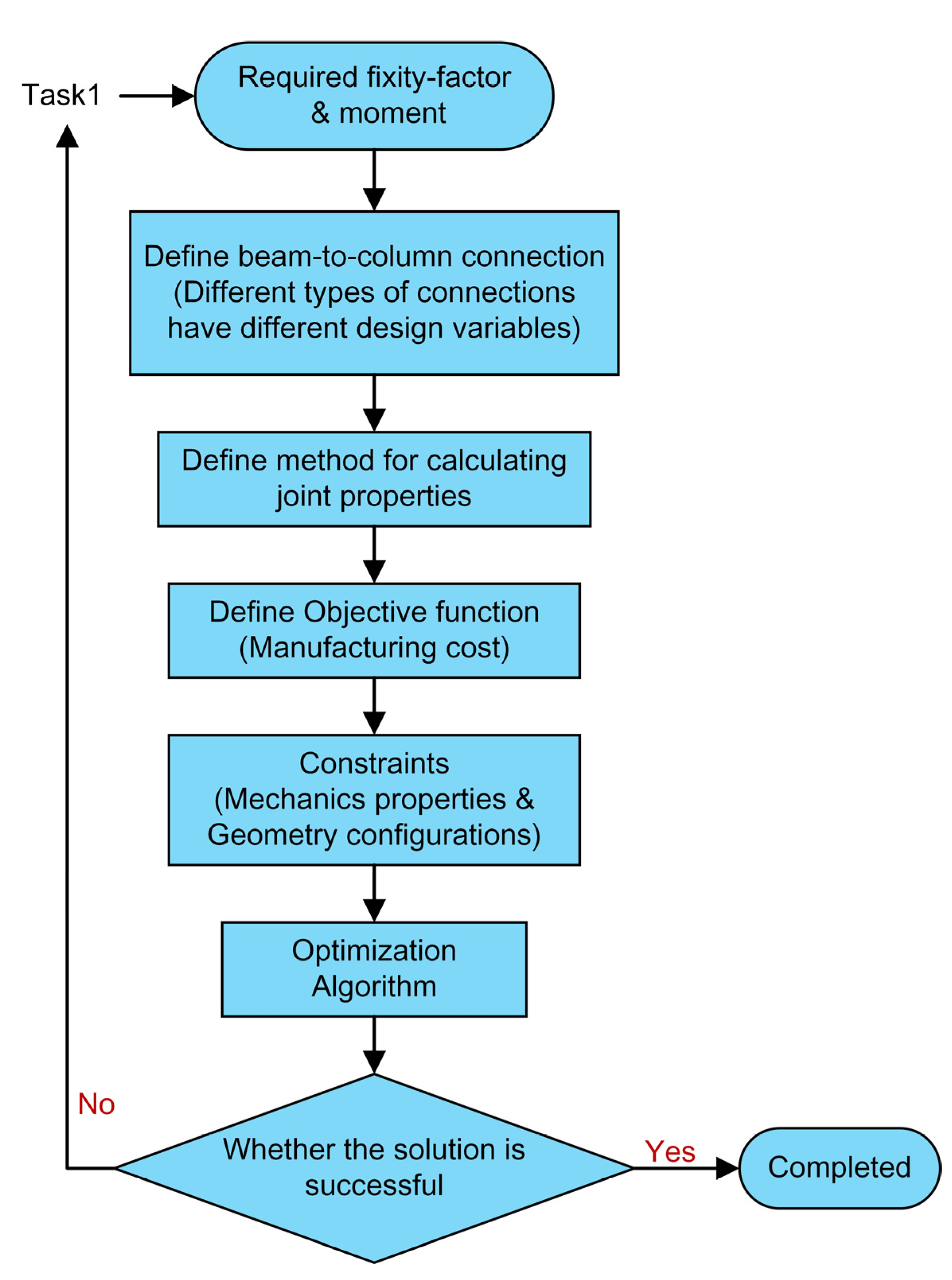
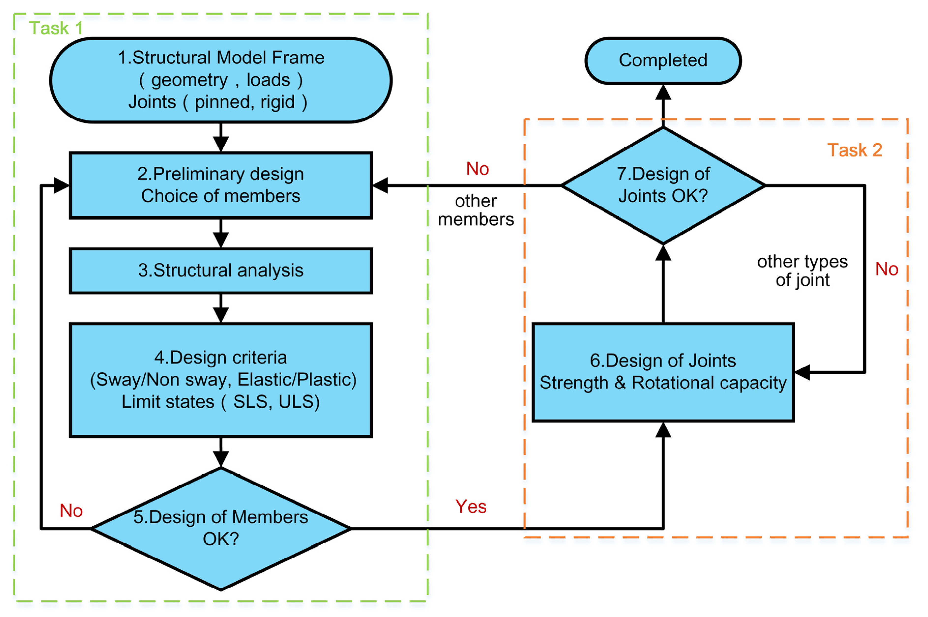
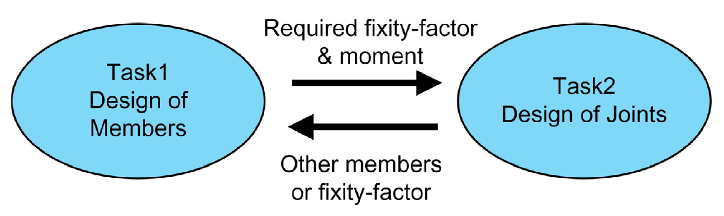
Therefore, an inverse design method has been developed in this paper aimed at addressing the aforementioned drawbacks encountered in the design of semi-rigid steel frames. The core of the approach is to link member design to joint design through joint performance requirements. In the structural analysis phase, both types and details of a joint are ignored, and the assumption that a joint is either pinned or rigid is generalized to a joint with a certain performance value. After completing the member design, a joint can be directly reconstructed by using the optimization algorithm subject to its required performance. This workflow is independent of joint types and can consider all joint parameters completely and implicitly. The innovative use of joint required performance greatly reduces the design variables that engineers need to control compared to geometric parameters, which enables the exploration of more competitive design results. In order to speed up the process of converting to a solution, this study also discusses the selection strategies of the initial value of the required connection stiffness from the characteristics of the connection. At the end of this article, two examples are presented to demonstrate the validity of the proposed method.

2. Methodologies

2.1. Traditional Design Method for Steel Frames

In traditional practice, the steel structure design is divided into member design and joint design two parts in succession [34]. The former refers to the selection of member profiles to meet the strength and serviceability requirements of the structure, while the latter refers to the design of joint details to fulfill the required mechanical performance.

Figure 1 shows the workflow of the entire design. The main feature of this process is that in task 1, the engineers do not need to care about any joint details when selecting the member profiles, and only pass limited data to task 2. Initially, the joints are assumed to be either pinned or rigid. After the member design is completed, the engineers provide the joint designers with the end reactions of beams and the assumptions of joints.

2.2. Proposed Design Method Suitable for Semi-Rigid Steel Frames

Before elaborating on the proposed method, it is necessary to understand two transformations that have been widely used for incorporating the joint properties into the structural model.

2.2.1. The Normalization of Joint Properties

Although the stiffness is usually used to characterize the rotational behavior of a joint, it cannot clearly reflect the rotational behavior of the joint in the structure, which is also related to the profile and length of the connected beam. Moreover, the stiffness ranges of different types of joints are different [35], which makes it impossible to represent each joint with a unified measure in the structural model.

Chen [2] adopted the conception of the end fixity-factor $r$ as in Equation (1), which presents the ratio of the end rotation of the connected beam, due to a unit end moment applied at the same end, to the corresponding rotation of the beam plus the joint.

$$r=\frac{1}{1+\frac{3E{I}_b}{S_{j,ini}{L}_b}}$$

(1)

where $E$ = Young’s modulus; ${\mathrm{s}}_{j,ini}$ = initial rotational stiffness of the joint; $I_{b }$ = moment of inertia of the connected beam; $L_b$ = length of the connected beam.

One advantage of this expression is that it normalizes the initial rotational stiffness for any joint type; 0 and 1 for a theoretical pinned and rigid joint, respectively, and intermediate values for semi-rigid joints. Therefore, in this study, an end fixity-factor is used to represent a joint in the structure model, rather than its stiffness.

For moment resistance of the joint, the moment capacity coefficient can be defined as Equation (2)

$$m=\frac{M_{j,rd}}{M_{b,pl}}$$

(2)

where $M_{j,rd}$ = moment capacity of the joint; $M_{b,pl}$ = plastic moment capacity of the connected beam.

2.2.2. Design Process

Return to Figure 1. In Step1, one joint is assumed to be either pinned or rigid, which converted to the end fixity-factor, is 0 or 1. In the final, in Step 7, the joint details should be checked to satisfy the assumptions made in Step1.

It is well known that the internal force and deformation response of a structure is essentially the result of stiffness and strength distribution of the components that make up this structure, no matter what profile the beams and columns have, or what details the joints have. If the details are implicit, any joint can be uniquely represented by a real number between 0 and 1. Therefore, it is easy to generalize the joint assumption in Step 1 of Figure 1 to a real number. While the joint design in Task 2 of Figure 1 can be converted to an inverse problem which reconstructs the joint details subject to the given required performance, including the required end fixity-factor and moment of the connected beam.

Here, a new design process suitable for semi-rigid steel frames is proposed, as shown in Figure 2. It can be seen that the new process is basically similar to the traditional one, except for some minor changes. In Task 1, there is no longer a need to focus on the types and details of the joints, but on their required performance. In Task 2, the joint design can be achieved by solving the inverse problem. The two tasks are linked together by the end fixity-factor and the required moment of the beam, as shown in Figure 3.

2.2.3. Reconstruction of the Joint

Pragmatically, the final configuration of one joint is unknown at the beginning of the design process. To obtain the identification of appropriate joint details from constraints and codes, an iterative process is required. However, this process is exhausting due to a large number of geometric and mechanical properties that have to be considered. Fortunately, it can be easily solved by optimization techniques, see Figure 4, by defining a cost function to measure how well a reconstruction fits the requirements, while simultaneously enforcing some additional characteristics and acting as regularization for the reconstruction process.

The main virtue of this method is that the entire solution process can be conducted automatically by a program without any manual processing. When necessary, various constraints can be defined to control the joint details. Designers only need to input the end fixity-factor and moment requirements, which greatly reduces the workload. Even better, it is a universal method applicable to any joint type, as long as the corresponding constraints and joint properties are calculated correctly.

The Standard formulation for the optimization problems is as in Equation (3):

$$\begin{gathered} Minimize C\left(x\right) \\ \mathrm{Subject} \mathrm{to} \{\begin{array}{c}{x}_i^l\le x_i\le x_i^u \left(i=1,\dots ,n_v\right)\\ h_j\left(x\right)=0 \left(j=1,\dots ,n_e\right)\\ g_k\left(x\right)\le 0 \left(k=1,\dots ,n_i\right)\end{array} \end{gathered}$$

(3)

where $x$ = vector of design variables; $C\left(x\right)$ = objective function; $h_j\left(x\right)$ = the $j_{th}$ equality constraint;$g_k\left(x\right)$ = the $k_{th}$ inequality constraint,$n_e$ = number of equality constraints, $n_i$ = number of inequality constraints, $x_i^l$ = lower bound of the $i_{th}$ design variable, $x_i^u$ = upper bound of the $i_{th}$ design variable, and $n_v$ = total number of design variables.

As the joint optimization design is not the focus of this research, only the core points are described briefly as follows. For more details, please refer to the literature [36,37].

• Objective function
  In order to obtain a more competitive design. The connection with lower manufacturing and materials costs should be selected. The calculation method proposed by Pavlovčič et al. [38] is adopted in this study.

2.

Constraints

• Joint properties
  Firstly, it is not practical to obtain a joint whose properties are exactly the same as the required. Secondly, the responses of the structure under loads are sensitive to the flexibility of the connections in it. Therefore, the errors between the properties of the ‘actual’ joint obtained by the optimization algorithm and the requirements should be within an acceptable tolerance.

  $$\left|1-\frac{S_{j,act}}{S_{j,req}}\right|\le \epsilon$$

  (4)

  $$\frac{M_{j,req}}{M_{j,act}}\le \theta$$

  (5)

  where $S_{j,act}$ = stiffness of the ‘actual’ joint obtained by optimization algorithm; $S_{j,req}$ = the joint required stiffness; $M_{j,req}$ = end moment requirement of the connected beam; $M_{j,act}$ = moment resistance of the ‘actual’ joint obtained by optimization algorithm; $\epsilon$ and $\theta$ are tolerances, and this study takes 0.05 and 1.0, respectively, which can meet the engineering needs.
• Geometry
  The joint geometry should meet the requirements of EN1998-1-8 [23]. These constraints are related to the bolt’s layout, including bolt diameter, edge distance, bolt spacing and assembly space.

3.

Calculation of joint properties

The initial rotational stiffness and moment resistance of the joint is calculated with reference to EN1993-1-8 [23] and SCI P398 [24].

4.

Optimization algorithm

A genetic algorithm [39] is adopted in this study due to its superiority in handling discrete, complex non-convex engineering problems.

3. Joint Modelling

3.1. Interaction of Web Panel

As displayed in Figure 5, a joint consists of a web panel in shear and a connection, the joint model should be able to take into account the behavior of these two parts under loads. In EN1993-1-8 [23] the beam element with end rotational springs is recommended, see Figure 6a. To take into account the shear interaction in the web panel, a transformation parameter $\beta$ is defined, and its precise value needs an iterative process, which inevitably increases the computation efforts. Other approaches, as shown in Figure 6b–d, developed the macro four-node joint element [40] or modeled the joint explicitly [41,42,43], which can take into consideration the behavior of the connection, as well as the panel zone in a complete way without the use of $\beta$. All internal forces and deformation that concur at the joint are considered automatically. Currently, the explicit ways can be implemented in modern structural software conveniently, thus, the scissor model is adopted in this study.

3.2. Constitutive Relationship of Rotational Spring

Although it would be correct to use a full joint moment–rotation curve in the structural model as the rotational characteristics of a semi-rigid joint are highly nonlinear, as shown in Figure 7, it is not convenient for engineering practice. Due to multiple parameters needing to be defined, more computing resources would be consumed. In practice, a simplified bi-linear model named the half initial secant stiffness method [44] can be used to approximate the moment-rotation characteristic of the joint.

$$S_{j,sec}=\frac{S_{j,ini}}{\eta }$$

(6)

where $S_{j,ini}$ = initial rotational stiffness of the joint; $\eta$ = reduction factor, which is 2.0 when the required moment is found to be no less than 2/3 joint resistance $M_{j,rd}$, and 1.0 otherwise.

4. Strategies for Selecting Initial Value of the Required Fixity-Factor

Theoretically, the fixity-factor of the connection can be any real number between 0 and 1, but choosing a good anchor point before starting would be beneficial to the design. The literature [33] used the fixity-factor of 0.66 as the starting point for the optimal design of semi-rigid steel frames, which comes from the conclusion that the most economical profile of the member can be obtained when the maximum moment in the beam equals half of the moment at the mid-span of this beam with two ends pinned [45]. However, this conclusion is based only on the analysis of isolated beams, without considering their behavior in the structure. Moreover, this method only focuses on the design of beams and does not provide any indication for the detailing of connections. Indeed, sometimes, there may be no available connection configurations for a predetermined end fixity-factor, as will be seen in the following analysis. Therefore, the characteristics of joints themselves should also be considered when determining the appropriate initial value of the fixity-factor.

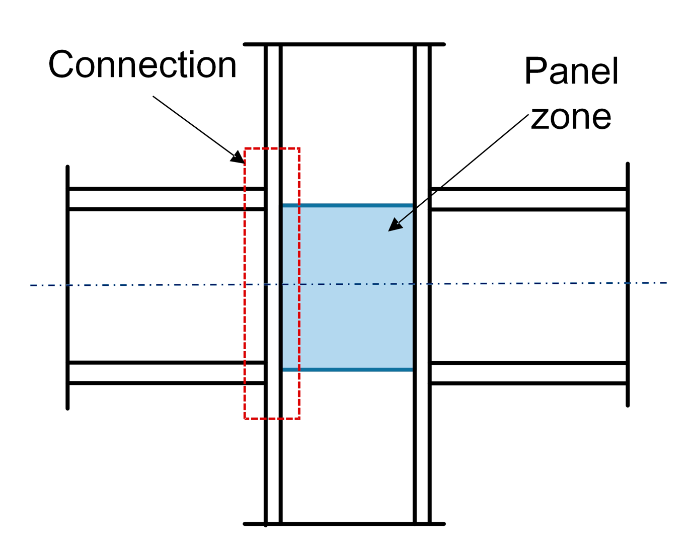
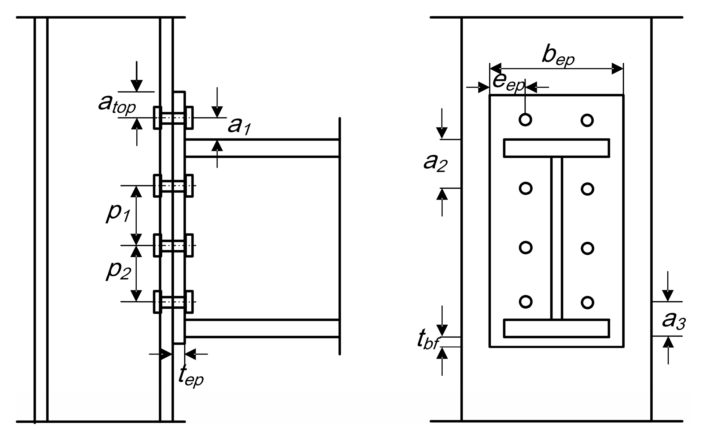
As mentioned in Section 3.1, the joint in this study is divided into two parts, the web panel and the connection, while the former is related to the profile of the column and its characteristics can be calculated directly if the column is pre-determined. Therefore, only the connection needs to be analyzed. A series of extended end-plate connections for different beam-to-column were analyzed, as listed in Table 1, including initial rotational stiffness, moment resistance and manufacturing cost. 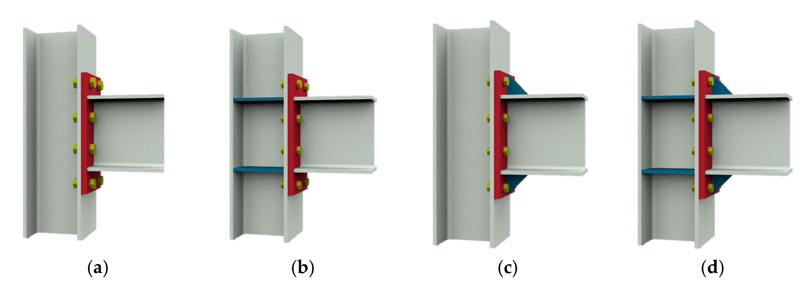All connections should be constructed in accordance with the requirements of EN1993-1-8 [23], mainly bolt spacing and edge distance limitations. To avoid weld failure, all welds are full strength. In order to cover as complete a variety of connection types as possible, whether or not to use continuity plates and end-plate ribs has also been considered. The variables of a connection are listed in Table 2 and the available configurations are displayed in Figure 8.

Table 1. Pairs of beam–column.

No.	Column 1	Beam 1
1	HE100B	IPE100
2	HE100B	IPE120
…	…	…
285	HE500B	IPE400
286	HE500B	IPE450
…	…	…
407	HE1000B	IPE550
408	HE1000B	IPE600

¹ HEB series for column, IPE series for beam. Refer to BS EN 10365:2017 [46] for the specific meaning of the labels, as well as dimensions of each section.

Table 1. Pairs of beam–column.

No.	Column 1	Beam 1
1	HE100B	IPE100
2	HE100B	IPE120
…	…	…
285	HE500B	IPE400
286	HE500B	IPE450
…	…	…
407	HE1000B	IPE550
408	HE1000B	IPE600

¹ HEB series for column, IPE series for beam. Refer to BS EN 10365:2017 [46] for the specific meaning of the labels, as well as dimensions of each section.

Table 2. Variables of a connection.

Project	Available
Plate thickness (mm)	10, 12, 14, 16, 20, 25
Steel grade 1	S275 (nominal yield strength of 275 Mpa)
Bolt thread d 2	M16, M20, M24, M30
Bolt class 3	8.8, 10.9
Rows of bolts 4	$\ge 3$
Edge distance 5	$1.2d_0~4t+40$
Bolt spacing	$\ge 2.2d_0$
Assembly space	$\ge 2.2d_0$
Continuity plates 6	Yes or No
Extended end-plate ribs 7	Yes or No

¹ As the strength of steel grade has little effect on the stiffness of the connection, this value can be arbitrarily selected. ² d is the nominal diameter of bolt thread and labeled in accordance with EN 14399-4:2015 [47]. ³ The nominal values of the yield strength and the ultimate tensile strength conforming to EN1993-1-8 Table 3.1 [23]. ⁴ There is only one row of bolts at the extended region of the end-plate, the total number of blot rows is not less than three, and the maximum value is related to the connected beam height, not a fixed value. ⁵ $d_0$ is the diameter of bolt hole, $t$ is the smaller thickness between the end-plate and the column flange. ⁶ Minimum value in the list of plate thickness and not less than the thickness of beam flange. ⁷ Minimum value in the list of plate thickness and not less than the thickness of beam web.

Table 2. Variables of a connection.

Project	Available
Plate thickness (mm)	10, 12, 14, 16, 20, 25
Steel grade 1	S275 (nominal yield strength of 275 Mpa)
Bolt thread d 2	M16, M20, M24, M30
Bolt class 3	8.8, 10.9
Rows of bolts 4	$\ge 3$
Edge distance 5	$1.2d_0~4t+40$
Bolt spacing	$\ge 2.2d_0$
Assembly space	$\ge 2.2d_0$
Continuity plates 6	Yes or No
Extended end-plate ribs 7	Yes or No

¹ As the strength of steel grade has little effect on the stiffness of the connection, this value can be arbitrarily selected. ² d is the nominal diameter of bolt thread and labeled in accordance with EN 14399-4:2015 [47]. ³ The nominal values of the yield strength and the ultimate tensile strength conforming to EN1993-1-8 Table 3.1 [23]. ⁴ There is only one row of bolts at the extended region of the end-plate, the total number of blot rows is not less than three, and the maximum value is related to the connected beam height, not a fixed value. ⁵ $d_0$ is the diameter of bolt hole, $t$ is the smaller thickness between the end-plate and the column flange. ⁶ Minimum value in the list of plate thickness and not less than the thickness of beam flange. ⁷ Minimum value in the list of plate thickness and not less than the thickness of beam web.

The analysis steps are as follows: Step 1: Initialize the list of available plate thickness, bolt sizes and bolt grades. Step 2: Select one pair of beam–column from Table 1. Step 3: Generate a mass of configurations with geometric constraints by sampling all design variables in Table 2 randomly. Most pairs of beam–column can have at least 3000 sets of valid data, with the expectation of a few that have fewer due to their section size limitations. Step 4: Calculate the initial rotational stiffness, flexural capacity and fabrication cost of all connections. Step 5: Go back to Step 2 and select the next pair of beam–column until all data in Table 1 are iterated.

Due to a large number of beam–column pairs in Table 1, it is impossible to display all data. Only the six sets of data in

Table 3. Six pairs of beam–column.

Column	Beam
HE140B	IPE200/IPE270
HE200B	IPE200/IPE270
HE600B	IPE200/IPE270

are presented to illustrate the analytical procedure. According to Section 2.2.1, the stiffness and moment capacity of the connection are converted into the fixity-factor and moment capacity coefficient, and the beam length is assumed to be 6 m. It is noted that this assumption will not affect the applicability of the conclusion, since the two connection properties analyzed here are relative values.

4.1. End Fixity-Factor vs. Moment Capacity Coefficient

The scatter density diagrams of fixity-factor vs. moment capacity coefficient are shown in Figure 9. Each point represents available joint details. The color band in the figure is used to mark the density of samples. Red indicates a higher number of valid configurations, while blue indicates a lower number.

In general, the rotational stiffness of a connection is positively correlated with its flexural capacity. That is, a connection with high rotational stiffness is often accompanied by a high flexural capacity. However, the relationship between them cannot be expressed in a simple function, because there is a range of moment capacity coefficient for a fixity-factor and vice versa, as can be seen in Figure 9. It can also be found that the connections under each pair of beam–column have their own applicable range of flexural capacity and fixity-factor range, which vary greatly. When the beam section is fixed, the upper limit of the flexural capacity of the joint increases with the increase in the column section. This is because the larger column section has thicker flanges that provide greater moment resistance. On the other hand, as the column section increases, the end-plate will have more room to accommodate larger bolts, conversely, the smaller column limits the maximum available diameter of the bolt.

The applicable boundaries regarding the rotational stiffness and moment capacity of semi-rigid connections would lead to a problem encountered in the design of semi-rigid steel frames. That is, there is no guarantee that available connection configurations would exist for any performance requirement. For example, when the required fixity-factor is 0.7, no connection configuration is available for those beam–column pairs in Figure 9, no matter how small the moment that is required. This is exactly the difference between semi-rigid connection and traditional connection, and the difficulty.

Another phenomenon is that the distribution density of scattered points varies from place to place, with a maximum variation that can be nearly two orders of magnitude. Moreover, all figures show that the density of valid configurations near the lower boundaries is sparse.

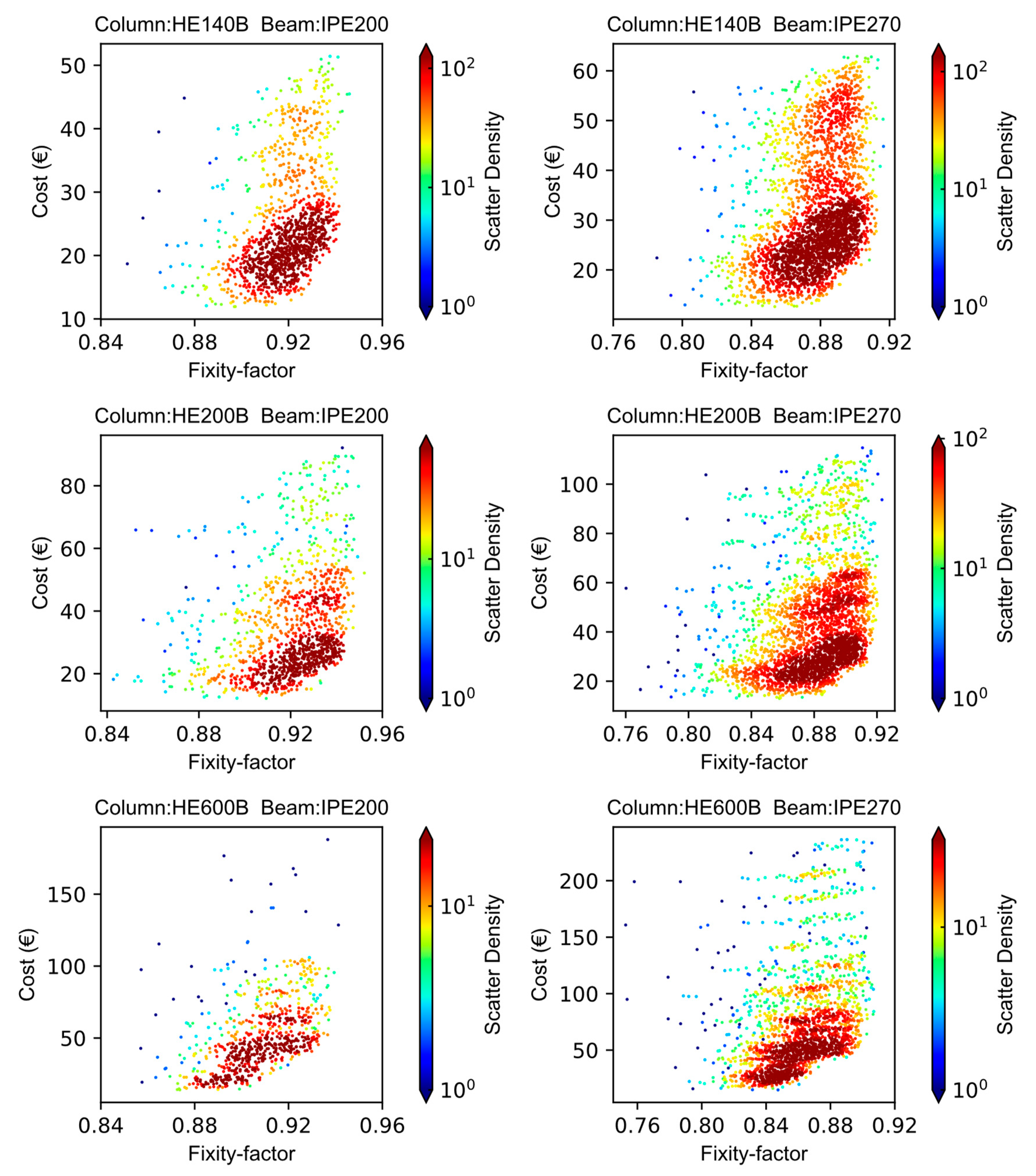
4.2. End Fixity-Factor vs. Manufacturing Cost

Figure 10 shows the scatter density diagrams of fixity-factor vs. manufacturing cost. There is a wide range of costs for any fixity-factor, with the highest being several times higher than the lowest. It is reasonable to choose a joint configuration that locates the periphery near the bottom of the longitudinal axis, as it is less expensive. Each set of data shows that the lowest cost is relatively stable within the first half of the fixity-factor range, exceeding this when the cost begins to increase significantly. Therefore, the selection of the joints should give priority to this region.

4.3. Recommendations

From the above discussion, it can be concluded that a good initial value of the required fixity-factor should meet the following conditions: (1) In the dense region of available configurations to increase the probability of a successful search; (2) In the region with less cost variation to obtain more economical results. Reasonably, the recommended starting value should be the intermediate value of the range regarding each beam–column, see Appendix A for more results.

5. Examples

In order to verify the effectiveness of the proposed method, two examples in the literature [33] are designed. European sections (i.e., HEB and IPE sections) are used for columns and beams, the material is steel S275, with a modulus of elasticity of 210,000 Mpa and a yield stress of 275 Mpa; the bolts are steel 10.9, with the nominal values of the yield strength and the ultimate tensile strength are 900 Mpa and 1000 Mpa, respectively. The second-order analysis with a buckling length factor of 1 is adopted here. To simplify the design, beams, columns, and connections are grouped into different groups, within which all members are unified. The asymmetrical extended end-plate connection in Figure 11 is used. The total number of rows of bolts is not less than three, and the specific number of rows depends on the design results. Thus, the variable p, may or may not exist.

After selecting the preliminary profile of each member based on experience, the starting value of the fixity-factor is set by referring to Section 4.3 and then the structural analysis is carried out. The starting value of the fixity-factor should be reset if any member section is changed during the iteration.

5.1. Frame A

The frame layout, loading conditions, and group numbers are shown in Figure 12. Beams on the same floor share the same profile and columns are supposed to be continuous. There are four types of connections and four types of web panels, labeled A, B, C, D, and pz₁, pz₂, pz₃, pz₄, respectively.

Table 4. Frame A: Member sections in each iteration.

	1	2	3	4
Initial	IPE200	IPE270	HE140B	HE160B
Iter1	IPE180	IPE270	HE140B	HE160B

and

Table 5. Frame A: Required joint properties in each iteration.

		${\mathit{r}}_{\mathit{r}\mathit{e}\mathit{q}}{ }^1$	${\mathit{S}}_{\mathit{r}\mathit{e}\mathit{q}}{ }^2$	${\mathit{m}}_{\mathit{r}\mathit{e}\mathit{q}}{ }^3$	${\mathit{M}}_{\mathit{r}\mathit{d},\mathit{r}\mathit{e}\mathit{q}}{ }^4$	${\mathit{S}}_{\mathit{a}\mathit{c}\mathit{t}}{ }^5$	${\mathit{M}}_{\mathit{r}\mathit{d},\mathit{a}\mathit{c}\mathit{t}}{ }^6$	Check
Initial	A	0.9	18,333.00	0.39	23.69	18,622.30	38.86	OK
	B	0.9	18,333.00	0.66	40.39	18,897.11	40.51	OK
	C	0.85	34,450.50	0.32	42.36	34,563.40	73.99	OK
	D	0.86	37,345.50	0.63	84.33	38,465.21	84.49	OK
	pz1	-	-	-	26.30	-	37.50	OK
	pz2	-	-	-	11.56	-	50.41	OK
	pz3	-	-	-	47.69	-	50.62	OK
	pz4	-	-	-	31.73	-	68.06	OK
Iter1	A	0.91	14,014.00	0.56	25.74	14,399.61	31.59	OK
	B	0.91	14,014.00	0.88	40.4	14,337.00	40.51	OK
	C	0.85	34,450.50	0.32	43.09	34,563.40	73.99	OK
	D	0.86	37,345.50	0.63	84.47	38,465.21	84.49	OK
	pz1	-	-	-	26.30	-	37.50	OK
	pz2	-	-	-	11.56	-	50.41	OK
	pz3	-	-	-	47.69	-	50.62	OK
	pz4	-	-	-	31.73	-	68.06	OK

¹ Required fixity-factor. ² Required initial rotational stiffness (kNm/rad). ³ Required moment capacity coefficient. ⁴ Required moment capacity (kNm). ⁵ Actual initial rotational stiffness (kNm/rad). ⁶ Actual moment capacity (kNm).

list the changes in the members’ section and joints required performance during iterations, respectively.

Table 6. Frame A: Final joint details (size in mm).

Joint	Beam	Column	Bolt	tep	bep	eep	atop	a1	a2	a3
A	IPE180	HE140B	M16 10.9	10	103	22	22	24	53	30
B	IPE180	HE160B	M16 10.9	10	139	24	22	24	31	52
C	IPE270	HE140B	M16 10.9	10	135	32	22	24	50	53
D	IPE270	HE160B	M16 10.9	12	135	27	22	24	45	53

lists the final joint details.

It can be seen from Table 5 that in the initial design, the maximum end moment requirement of connection A is 23.69 kNm, which is far less than the actual moment resistance of 38.86 kNm. Although a new joint with less moment resistance can be obtained by reducing the end fixity-factor, the benefit is limited since the start value of the end fixity-factor is set at a position with small connection cost variation, as described in Section 4.2. Further analysis shows that connection A has a low $m_{req}$, which means that the moment resistance of the connected beam has a large margin as well as the shear resistance of the web panel in pz₁ and pz₂. Therefore, reduce 1# beam to IPE180 and enter the iter1 to obtain the solution.

5.2. Frame B

The frame layout, loading conditions, and group numbers are shown in Figure 13. There are six types of connections and five types of web panels, labeled A, B, C, D, E, F, and pz₁, pz₂, pz₃, pz₄, pz₅, respectively. Different from the literature [33], two end connections of 4# beam share the same configuration in this study. The joint with different beam heights on two sides of the column and the mean of beam heights on both sides are taken to calculate the properties of the web panel.

Table 7. Frame B: Member sections in each iteration.

	1	2	3	4	5	6
Initial	IPE160	IPE220	IPE240	IPE360	HE140B	HE180B
Iter1	IPE200	IPE240	IPE270	IPE300	HE140B	HE180B
Iter2	IPE200	IPE240	IPE270	IPE330	HE140B	HE180B

and

Table 8. Frame B: Required joint properties in each iteration.

		${\mathit{r}}_{\mathit{r}\mathit{e}\mathit{q}}$	${\mathit{S}}_{\mathit{r}\mathit{e}\mathit{q}}$	${\mathit{m}}_{\mathit{r}\mathit{e}\mathit{q}}$	${\mathit{M}}_{\mathit{r}\mathit{d},\mathit{r}\mathit{e}\mathit{q}}$	${\mathit{S}}_{\mathit{a}\mathit{c}\mathit{t}}$	${\mathit{M}}_{\mathit{r}\mathit{d},\mathit{a}\mathit{c}\mathit{t}}$	Check
Initial	A	0.88	10,036.95	0.48	16.38	10,287.53	28.67	OK
	B	0.9	12,318.08	1.21	41.22	null 1	null	NO
	C	0.83	14,200.32	0.96	75.43	null	null	NO
	D	0.84	32,165.44	0.15	11.66	31,562.89	52.47	OK
	E	0.82	27,910.75	1.40	109.86	null	null	NO
	F	0.81	72,963.95	0.38	109.42	71,884.07	130.45	OK
	pz1	-	-	-	19.73	-	30.00	OK
	pz2	-	-	-	25.00	-	63.79	OK
	pz3	-	-	-	19.64	-	45.00	OK
	pz4	-	-	-	2.26	-	104.38	OK
	pz5	-	-	-	128.46	-	104.38	NO
Iter1	A	0.86	18,769.50	0.28	12.69	18,750.41	38.31	OK
	B	0.84	16,041.38	0.67	40.46	16,529.29	41.33	OK
	C	0.86	25,090.50	0.80	80.40	25,814.54	81.24	OK
	D	0.79	34,305.75	0.03	4.08	34,482.57	67.13	OK
	E	0.78	32,331.89	0.90	119.21	null	null	NO
	F	0.82	39,988.67	0.76	131.11	null	null	NO
	pz1	-	-	-	22.72	-	37.50	OK
	pz2	-	-	-	25.00	-	69.59	OK
	pz3	-	-	-	19.64	-	50.62	OK
	pz4	-	-	-	15.87	-	86.98	OK
	pz5	-	-	-	128.46	-	173.96	OK
Iter2	A	0.86	18,769.50	0.27	12.54	18,706.87	38.98	OK
	B	0.84	16,041.38	0.67	40.84	16,529.29	41.33	OK
	C	0.86	25,090.50	0.80	80.24	25,805.87	81.07	OK
	D	0.79	34,305.75	0.03	4.26	34,356.08	66.03	OK
	E	0.78	32,331.89	0.87	115.17	33,298.64	115.22	OK
	F	0.81	52,820.53	0.55	120.87	53,601.33	123.12	OK
	pz1	-	-	-	16.01	-	37.50	OK
	pz2	-	-	-	23.68	-	69.59	OK
	pz3	-	-	-	12.41	-	50.62	OK
	pz4	-	-	-	10.18	-	95.68	OK
	pz5	-	-	-	134.20	-	191.36	OK

¹ “Null” indicates that there are no suitable connection details under the given performance requirements.

list the changes in the members’ section and joints required performance during iterations, respectively.

Table 9. Frame B: Final joint details (size in mm).

Joint	Beam	Column	Bolt	tep	bep	eep	atop	a1	a2	a3	p1
A	IPE200	HE140B	M16 10.9	10	103	22	22	24	51	45	- 1
B	IPE200	HE180B	M16 10.9	10	129	22	22	25	53	39	-
C	IPE240	HE180B	M16 10.9	12	141	22	22	24	38	47	77
D	IPE270	HE140B	M16 10.9	10	135	33	22	24	54	48	-
E	IPE270	HE180B	M20 10.9	20	178	29	28	45	62	62	75
F	IPE330	HE180B	M16 10.9	14	160	31	22	36	53	41	102

¹ “-” indicates that there is no such parameter. For example, connection A has only three rows of bolts while connection C has four rows of bolts.

lists the final joint details.

As can be seen from Table 8, in the initial design the maximum moment requirements of connection B and E both exceeded the plastic moment capacity of the connected beams too much, and the maximum moment requirement of connection B is also basically close to the plastic moment capacity of 2# beam, which results in no applicable connection configurations for them. Although releasing the end fixity-factor can reduce the end moment requirement of the beam, an appropriate connection has never been found. Therefore, it is considered to enlarge the section of 1#, 2#, and 3# beams, respectively. In contrast, the 4# beam has a large margin as well as connection F, and it is reasonable to replace this beam with a smaller one. Although the result at pz₅ indicates that the shear resistance of the web panel is insufficient, it is not intended to increase the size of the column here, but only to strengthen its web by welding a double plate. In iter1, there is no suitable configuration for connections E and F. A larger profile for the 4# beam is considered. Entering iter2, the result can be obtained.

6. Conclusions

This paper presents a feasible design method for semi-rigid steel frames, whose main advantage compared to previous methods, is that the joint details are implicit in the whole process and engineers do not need to have a deep understanding of the design of semi-rigid joints and leave the heavy work to the algorithm. By focusing on exploring the performance requirements of the joints in the structure, a more competitive design can be discovered. The most fundamental aspects and principles of this method are established in this paper, including the framework for the design process, the application of reconstructing connection details based on performance requirements, and strategies for selecting the initial fixity-factor of the joints. The following conclusions can be drawn:

• The workflow of the proposed method is basically the same as the traditional steel structure design and is easy to introduce to engineers. The members and joints are designed separately but closely linked by the joints’ required performance, which informs the engineers of the direction of adjustment more clearly than the geometric parameters of the joints during structural design.
• The innovative idea of reconstructing the joint details by using an optimization algorithm to meet the joint required performance realizes the black-box design of the joint. With the constraints of rotational stiffness and moment resistance requirements, the joint details can be obtained quickly, which avoids the uncertainty and complexity of the forward design from geometric parameters to properties and significantly improves the design efficiency.
• The characteristics and manufacturing costs of a series of beam-to-column connections have been analyzed in this study. It is found that there are certain stiffness boundaries for joints under various beam–column. The intermediate value at the beginning of the design is suggested, as this position corresponds to a high validity ratio and low-cost variation of the configurations. The invalid design of semi-rigid joints is effectively reduced, and the solving efficiency is improved.
• Lastly, it is worth mentioning that the examples only discuss the application of extended end-plate connections and CM. However, due to the independence of the joint design, it can be easily extended to other joint types, provided that relevant design criteria and characteristic calculation methods are defined.