Abstract
The associations between various design variables affecting the visual performance of responsive facade systems are investigated in this study. First, we propose a data-driven approach to study practical aspects of illuminance optimization for responsive facades. In this approach, the hourly indoor illuminance data are combined with the location information to generate an objective function. This function is then utilized to evaluate the visual performance of responsive facade systems by matching a variety of facade angle movements to hourly sunshine patterns. Next, statistical tests were deployed to evaluate the role of design variables in different scenarios. The results provide detailed information about the design variables and their effects on visual comfort at 0.05 significant levels. On average, facade angles, facade configurations, facade orientations, and facade locations were significant in 100%, 41%, 87%, and 45% of different possible combinations of scenarios/variables, respectively.
1. Introduction
A building facade system is one of the most important contributors to occupant comfort [1]. The performance of building facades contributes to 17 percent of occupants’ visual comfort and 58 percent of occupants’ thermal comfort [2,3]. Traditional facades, as static systems, are incapable of altering their performance over time in response to frequent variations in weather [4,5,6]. The performance of dynamic facades developed by advanced technologies can improve the limited response of static facades [7,8,9]. Facade systems have the potential to change their function, features, and behavior over time in response to repeated weather changes using advanced control technologies [10]. If the design variables for a responsive facade system are optimized for specific objectives, such as improved occupant visual comfort [11], the system can perform optimally. Occupants’ visual comfort optimization is not a straightforward process [12]. The number of variables involved and the complexity of interactions among the variables make the optimization problem a difficult task for designers [13,14].
In the design process, three types of design variables must be considered: active design variables, passive design variables, and environmental variables [13]. Active design variables such as louver angles, the facade porosity, and facade granularity can adjust the response to external stimuli and interior elements [9]. In contrast, passive design variables remain constant in response to external stimuli and interior elements, including infiltration, window-to-wall ratio, glazing types, and wall insulation [15]. Furthermore, parametric study of environmental variables such as climate zones, building locations, facade orientations, and facade configurations can be implemented to develop multiple design scenarios [14].
Limited past studies developed mathematical models that incorporate active, passive, and environmental variables to optimize visual comfort in responsive facades [13,14,15]. However, no study has investigated the impact of the design variables and their associations with the optimization function in responsive facades.
In this study, we present a double stage framework for investigating the associations between various design variables affecting the visual performance of responsive facade systems. First, we focused on louver adaptation angles in horizontal and vertical facade configuration. An objective function for obtaining optimal indoor illuminance is introduced, utilizing hourly adaptation angles. Compared to the previous objective functions, the proposed function can support all possible occupant activities with the required illuminance ranges. Moreover, the proposed function can deliver an optimal solution even when multiple activities are conducted in the room in different timeframes. The brute force search algorithm is implemented to decide the optimum hourly angles for various facade configurations, orientations, and locations/climates. To find the maximum indoor illuminance, the proposed optimization function is calculated for increments of the facade variables and time.
In the second stage, a proposed three-step framework is implemented to investigate the associations of various design variables with the optimal solution affecting the visual performance of responsive facade systems. The three main steps of the proposed framework are (1) defining scenarios, (2) performing statistical tests, and (3) evaluating the test results, which determines the association of the variables with the optimal solution.
Since the proposed framework yields the optimum angles as its main outcome, the optimum angles are inputted in a facade control system. This potentially could not only improve control latency, but also reduce computational cost. However, it should be explicitly noted that the cost of the hardware and required computational power were not considered in this study and would vary depending on the building specifications.
2. Materials and Methods
2.1. Experimental Settings
A typical office room was designed using Rhinoceros version 6.0 developed by Robert McNeel & Associates (Seattle, WA, USA). The dimensions of the designed office were 4.0 m wide, 9.0 m deep, and 3.0 m high. The typical daylight zone is about 7.0 m deep from the window wall in common office spaces [16]. The thickness of walls, ceiling, and flooring elements are 0.15 m, 0.12 m, and 0.12 m, respectively. The depth of the office was chosen to be larger than the typical depth so that the effect of daylight remains visible for all variables [17]. Natural light was considered as the only source of light in the office room, with no artificial lighting inside. This simulated office room had a window opening of 2.6 m width and 3.6 m length. The window was made from double-glazed, clear glass with a visible light transmittance of 76% that was installed on the small side of the office room. The window-to-wall ratio before applying the responsive facade system was 78% (floor area = 36.0 m2 and window area = 9.36 m2 representing a 26% glazing to floor ratio).
Using the Grasshopper modeling tool, a responsive facade system was simulated parametrically and applied to the office window. The simulated office room could be rotated to face the four main cardinal directions (N, W, S, E) in order to create various design scenarios.
The horizontal and vertical louver angles were able to be rotated hourly from −90 degrees to +90 degrees in response to daylight patterns during the day. Horizontal and vertical louvers moved in a clockwise direction from −90 degrees to +90 degrees. The movement of louvers was divided into 60 steps with increments of 3 degrees. The designed facades considered for simulation consisted of 7 horizontal and 7 vertical louvers with dimensions of 3 m × 0.26 m × 0.18 m, as shown in Figure 1. The distances between louvers in the horizontal configuration were 0.40 m and in the vertical configuration were 0.50 m when louvers were fitted on 0 degrees. It is assumed that the louvers were built from diffuse metal provided by DIVA, which corresponds to Radiance parameters of 0.9 specularity, 0.175 roughness, and 0.175 reflectance (RGB) in the DIVA plug-in.
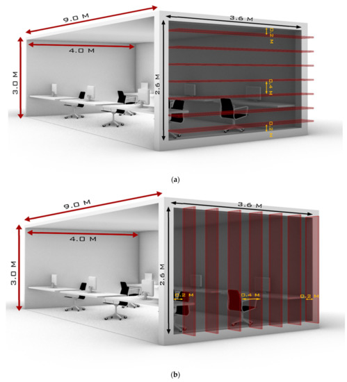
Figure 1.
Standard south-facing office space with workstations. (a) Horizontal responsive louvers. (b) Vertical responsive louvers.
The DIVA daylight-modeling plug-in was utilized to measure indoor illuminance and its corresponding visual metric of Useful Daylight Illuminance (UDI). The DIVA is one of Grasshopper’s plug-ins, which assists Grasshopper in conducting sustainability simulations, such as daylight analysis. Radiance is the core of the DIVA engine and was previously validated by other researchers [18,19,20,21,22,23,24,25]. It has been proven by Reinhart and Walkenhorst that Radiance-based simulation methods are able to efficiently and accurately model complicated daylighting elements [18]. It has also been demonstrated by Ng et al. [18] that Radiance can be used to predict the internal illuminance with a high degree of accuracy. Additionally, Yoon et al. [19] have stated that Radiance is validated computational software and is well known to provide reliable prediction results under various sky conditions. Furthermore, Reinhart and Andersen have shown that translucent materials can be modeled in Radiance with even higher accuracy than was demonstrated earlier [20,21,22,23,24,25].
A grid-based metric of indoor illuminance was developed by defining 220 sensors located over a horizontal grid surface with a height of 0.8 m from the office floor, which was within the average height of a work surface in an office. In both directions of the surface, sensors were spaced approximately every 0.43 m apart. The interior of the office room was simulated using standard Radiance materials that included a generic floor with 20% reflectance, a generic ceiling with 70% reflectance, generic interior walls with 50% reflectance, and generic furniture with 50% reflectance.
It was assumed that the office would be occupied daily from 8:00 a.m. to 6:00 p.m. without daylight savings time. IESNA’s new Lighting Measurement IES LM-83-12 was in agreement with the occupancy schedule [17]. It was assumed that six workspaces would be occupied during occupancy hours. The occupants would be performing regular office work, including working on computers. The clear sky with the sun was assumed as sky conditions. Typical annual meteorological data provided as an EnergyPlus Weather File (EPW) by the U.S. Department of Energy were utilized for the selected cities/climate zones. Three design scenarios were considered: (1) no louvers/no shade, (2) fixed horizontal and vertical louvers with zero-degree angle, and (3) responsive horizontal and vertical louvers with hourly optimum angles, as shown in Figure 2. These scenarios were repeated parametrically for four facade orientations (N, W, S, E) and different facade locations/climate zones.
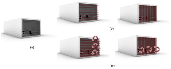
Figure 2.
The three design scenarios. (a) No shade/no louvers. (b) Fixed louvers with zero-degree angle. (c) Responsive louvers with hourly optimum angles.
Four cities from different climate zones in the United States, namely, Miami (FL), Phoenix (AZ), Boston (MA), and Milwaukee (WI), were selected using K-cluster analysis along with an elbow method [26,27]. Annual meteorological data of the selected cities were adopted to simulate the hourly indoor illuminance associated with the multiple scenarios considered. Based on the ASHRAE classification, Miami and Phoenix represent the very Hot-Humid (1A) and Hot-Dry (2B) climates, respectively. Boston and Milwaukee represent Cool-Humid (5A) and Cold-Humid (6A) climates, respectively [28].
Hourly indoor illuminances were calculated at 220 predefined sensors for every 8760 h of a year, while the responsive louver angles were parametrically changed incrementally from −90 to +90°. The measurements were repeated for four facade orientations, horizontal and vertical facade configurations, and four cities/climate zones. The simulations ran 37,843,200 times to calculate and stored raw indoor illuminance values at 8,325,504,000.
The stored output data of the DIVA plug-in were transferred and stored in the Postgres-SQL database. Then, R software was utilized to apply the brute force search algorithm based on the proposed objective function to find the optimum louver angles [29,30,31]. After calculating indoor illuminance, UDI is calculated as a metric, which represents both indoor illuminance level and discomfort glare in one scheme, as widely utilized in the field. Figure 3 shows the flow and execution of the data in the simulation.
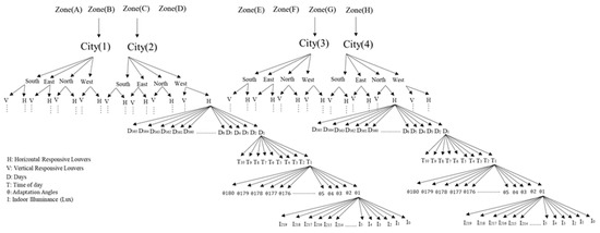
Figure 3.
Structure of the simulation runs.
2.2. The Proposed Framework—Stage 1
The UDI is a measure of the annual light quantity accessible in a certain interior space. The annual average of UDI may be used to evaluate the annual performance of a facade. The UDI metric, which depends on both active and passive variables, is considered as a dependent variable for establishing an objective function [28,29,30,31]. The UDI is calculated not only as lower and upper thresholds but also as a useful value depending on the range of illuminance. The lower and upper thresholds and the useful value of UDI are denoted as UDIunderlit, UDIoverlit, and UDIuseful, respectively [32]. In general, UDI is defined as a weighted average as follows [30]:
where ti is the time when the illuminance E is calculated, and wfi is the weighting factor, which depends on the range of the calculated illuminance E. It should be noted that the weighting factor wfi is selected based on the range of the calculated illuminance E. For instance, as shown below, for the upper threshold, UDIoverlit is calculated as below after wfi is selected depending on how the illuminance E value compares to the upper limit of illuminance specified in standards:
In a similar way, the lower threshold UDIunderlit is calculated as:
Similarly, UDIuseful is calculated as:
To optimize indoor illuminance, an objective function is established in the following general form as:
In this study, an objective function with active variables that can adapt the hourly daylight pattern is proposed. The illuminance includes the useful, overlit, and underlit ranges as the function constraints. These constraints divide interior space into three zones with three different levels of indoor illuminance appropriate for three distinct human activities. The goal of the proposed objective function is to increase the area of useful range for the different human activities and to decrease the area of undesirable ranges.
Two configurations of responsive facades, facades with horizontal louvers and facades with vertical louvers, were considered. The selected configurations are the most influential among various types of responsive facades with high visual performance in facade orientations [33,34,35,36].
Let represent a specific set of human activities in a desired range of illuminance. H = {h1, h2, …, hk} denotes hour of the day, and indicates the indoor illuminance for a specific point x located in the room for a louver angle of . Then, depending on whether or not the value of lays on one of the desired ranges, a new indication function is calculated for a specific point of x in the room and louver angle by using Equation (3):
It should be noted that indicates some indoor illuminance since it is based on the value of . Depending on the importance of the human activities, which correspond to the illuminance ranges defined in , a weighting factor W may be defined in a matrix form as:
The rows of the weighting factor are associated with the different human activities as defined in . Thus, there are as many columns as the numbers of human activities as defined in and denoted by . The weighting factors of columns are associated with the different hours of the day as defined in H and denoted by |H| for which is calculated. The hours considered were from 8:00 a.m. to 6:00 p.m.
For a given hour of h, the weighting factors associated with the human activities are obtained by calculating a weighted average of values of the indication function for the entire points in the room. As shown in Equation (8), the weighted average can be considered as a new indoor illuminance function and be presented as a new metric, sAUDIh:
where denotes the total number of points in the room.
The final objective function, AUDI, which is a function of the point x, the louvre angle , and the hour h, is computed by adding the calculated sAUDIh for all the hours, as presented in Equation (9):
2.3. The Proposed Framework—Stage 2
While the first stage of the framework aims to find the optimum angle by using Equation (6), the second stage investigates the role of various input variables in the optimum daylight illuminance. There are three steps in this stage, entitled scenario generation, hypothesis test assignment, and hypothesis test conduction and evaluation, as shown in Figure 4. The scenario generation step includes the following:
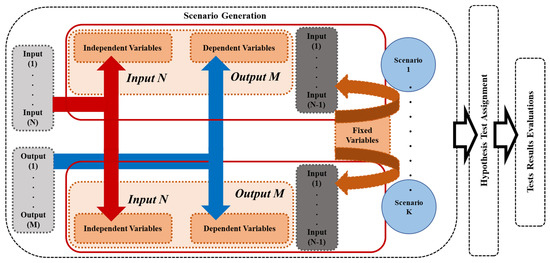
Figure 4.
Stage 2 of the framework.
- A dependent variable is selected from the visual comfort and maximum visual comfort calculations of Equation (9).
- An independent variable is chosen from active variables or environmental variables.
- Other input variables are fixed at specific values.
As an example, in order to investigate whether the office orientation impacts the values of the maximum visual comfort, the office orientation and the maximum hourly visual comfort are considered as the independent variable and dependent variables, respectively.
Each design scenario needs a specific statistical test based on the type of the independent and dependent variables. Therefore, the second step assigns a statistical test from the list of available statistical tests based on the different experimental settings (scenarios) and the type of the dependent and independent variables. The statistical tests available for this step include ANOVA, the Kruskal–Wallis, and Chi-squared [37,38,39].
Finally, the third step evaluates the results of the statistical test based on the obtained p-value, which measures the difference between the involved populations in the conducted test. A p-value greater than 0.05 indicates statistical insignificance. Thus, if the p-value calculated was below 0.05, the result was considered as statistically significant.
All statistical analyses were carried out using R v.3.4.0 [40]. The complete list of the variables is provided in Table 1. Using the statistical tests presented in Table 1, the impacts of several independent variables on visual comfort were investigated. These independent variables include adaptation angles, type of rotational motion of the louvers (horizontal or vertical), orientations of responsive facade systems, and the range of the rotational angles of the louvers’ motion. Some of the independent variables mentioned are active variables and others are environmental.

Table 1.
Experimental settings for scenario generation.
3. Results
The percentage values of the indoor illuminance function %sAUDIh for the three different human activities of , , and associated with the three different illuminance ranges and for both horizontal and vertical louvers on two specific days of 21 June and 21 December are presented in Table 2, Table 3, Table 4 and Table 5. The three different human activities of s1, s2, and s3 associated with the three different illuminance ranges are introduced in Equation (7).
Table 2.
Hourly optimum angles and the associated sAUDIh for three different human activities of , , and and four facade orientations calculated for 21 June-Phoenix-Horizontal louvers.
Table 3.
Hourly optimum angles and the associated sAUDIh for three different human activities of s1, s2, and s3 and four facade orientations calculated for 21 June-Phoenix-Vertical louvers.
Table 4.
Hourly optimum angles and the associated sAUDIh for three different human activities of , , and and four facade orientations calculated for 21 December-Phoenix-Horizontal louvers.
Table 5.
Hourly optimum angles and the associated sAUDIh for three different human activities of , , and and four facade orientations calculated for 21 December-Phoenix-Vertical louvers.
As shown in Table 2, at 12:00 p.m. on 21 June, the percentage value of sAUDIh associated with the target range of (where illuminance is between 300 Lux and 1000 Lux) is calculated as 36%. This value indicates that 36% of the working space area had the desired indoor illuminance (as specified for human activity) if an optimum angle of −32 degrees was chosen for south-facing horizontal louvers for that specific time of the year.
The hourly optimum angles and sAUDIh associated with ranges , , and for all the locations investigated including Miami, Phoenix, Boston, and Milwaukee on 21 June for the entire facade orientations are shown in Table 6, Table 7, Table 8, Table 9, Table 10 and Table 11.
Table 6.
The hourly optimum angles and their associated %sAUDIh on 21 June in Miami−Horizontal Louvers.
Table 7.
The hourly optimum angles and their associated %sAUDIh on 21 June in Miami-Vertical louvers.
Table 8.
The hourly optimum angles and their associated %sAUDIh on 21 June in Boston-Horizontal louvers.
Table 9.
The hourly optimum angles and their associated %sAUDIh on 21 June in Boston−Vertical louvers.
Table 10.
The hourly optimum angles and their associated %sAUDIh on 21 June in Milwaukee-Horizontal louvers.
Table 11.
The hourly optimum angles and their associated %sAUDIh on 21 June in Milwaukee−Vertical louvers.
Figure 5 shows the percentage values of sAUDIh associated with ranges , , and for a south-orientated office in Phoenix on 21 June when the responsive louvers were set at an optimum angle of 32 degrees. Furthermore, the percentage values of sAUDIh on 21 June associated with ranges , , and are illustrated in Figure 6a–c for four facade orientations (N, W, S, E).
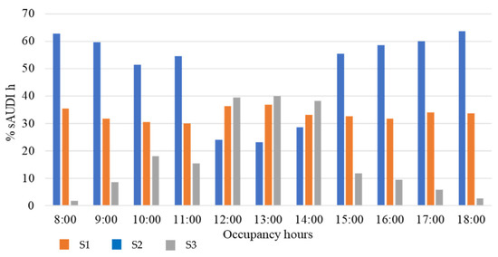
Figure 5.
The %sAUDIh for three different human activities of , , and for south facade orientations calculated for 21 June in Phoenix.
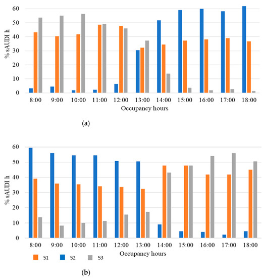
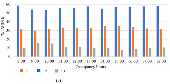
Figure 6.
The %sAUDIh associated with s1, s2, and s3 for horizontal responsive louvers with optimum angles for south, east, north, and west facades on 21 June in Phoenix. (a) East, (b) West, (c) North.
Additionally, the visual representation of the estimated indoor illuminance in the office considered is depicted in Figure 7. It is observed that the area which experiences the targeted illuminance range s1 increases as a responsive facade with an optimum angle is utilized as opposed to a fixed louver system.
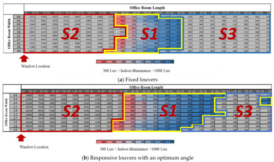
Figure 7.
Indoor illuminance distribution (on the assumed horizontal grid surface considered) in the office categorized with the three ranges of indoor illuminance s1, s2, and s3 for (a) fixed louvers and (b) responsive louvers set with the optimum angle utilized at noon on 21 June for south facade in Phoenix.
To examine the significance of the optimum adaptation angle (as an active variable) on the maximum visual comfort, 384 scenarios were generated. One-way ANOVA statistical tests were performed, and the results are shown in Table 6. The p-values less than 0.05 demonstrate significant differences between the facade of fixed louvers of a 0-degree angle (base case) and the vast majority of the responsive facades of horizontal configuration for all orientations examined in the city of Phoenix. This suggests that applying the optimal adaptation angles to the responsive facade of horizontal configuration leads to more desirable indoor illuminance for the majority of cases. The p-value of greater than 0.05 in Table 12 suggests that there were no significant differences between the responsive facade with optimum adaption angles and the responsive facade with fixed louvers of a 0-degree angle. This case is associated with the month of December for the south orientation and suggests that for this specific time of the year, and for such an orientation, applying optimum adaptation angles does not lead to more desirable indoor illuminance as compared to the fixed facade.
Table 12.
Significant differences between fixed facade (FF) and responsive facade (RF) with horizontal louvers.
A similar approach was used for the responsive facade of vertical configurations for the city of Phoenix for all main orientations. It was observed that applying optimum adaptation angles led to more desirable indoor illuminance for facades of vertical configuration.
One-way ANOVA statistical tests were conducted for four cities of Miami, Phoenix, Boston, and Milwaukee in both horizontal and vertical layouts.
To evaluate the significance of rotation direction of the louver angle, both optimum positive and negative adaption angles were considered as the independent variables. Different orientations and cities were considered for both positive and negative adaptation angles to generate 32 scenarios for both horizontal and vertical louvers. Then, Chi-squared tests were utilized. The results for Phoenix are shown in Table 13, which demonstrates that Chi-squared tests delivered significantly low p-values (p < 0.05), indicating there were significant differences between the optimum positive and negative adaptation angles for both horizontal and vertical louvers in all four facade orientations.
Table 13.
Significant differences between positive and negative optimum adaptation angles in the city of Phoenix.
To study the role of horizontal versus vertical louvers, 192 distinct scenarios were considered and one-way ANOVA tests were performed. The results are shown in Table 14, providing different ranges of p-values depending on month of the year. Thus, the difference between horizontal and vertical louvers is significant for only those months of the year when the p-value is below 0.05. For the remaining months, the difference was found to be insignificant.
Table 14.
Significant differences between horizontal and vertical louvers for the months of January, February, June, July, November, and December.
To determine the significance of the four key orientations of building facades, 96 scenarios were considered that included both horizontal and vertical louvers. Kruskal–Wallis tests were applied to the scenarios and the results are shown in Table 15, which shows significant differences for all four facade orientations. The tests were repeated for four different cities, and similar results were achieved.
Table 15.
Significant differences among different building orientations including south-facing, north-facing, east-facing, and west-facing in Phoenix.
4. Conclusions
In this study, we developed an objective function and a data-driven approach to investigate the contribution of different design variables to the visual performance of responsive facades. A computer model of an office with specific responsive facades (in the form of louvers) was constructed as an architectural space. For a specific hour of a day, the louvers were set to a specific adaptation angle, and a simulation was conducted to estimate the indoor illuminance. For the same selected hour, the simulation was repeated for a range of different adaptation angles to estimate the associated indoor illuminance. The data collected on indoor illuminance were fed into the proposed objective function to deliver the optimum adaptation angle for the selected hour. This process was repeated for all hours of a day and all days of a year. The study was also repeated for several design variables, including the location of the office, orientation of the office, and the facade’s configuration being vertical or horizontal.
Statistical tests were implemented to investigate the significance of the design variables on the visual comfort under different scenarios. In limited cases, and under specific circumstances, some design variables were found to be insignificant.
The results of this study indicate that obtaining and deploying optimum adaptation angles could lead to significantly desired levels of visual comfort. Implementing the proposed approach could help designers achieve higher levels of visual comfort, although the specifics of the design variables (such as location, orientation, and facade configuration) must be considered during the design process.
Author Contributions
N.H.M., conceptualization, methodology, software, draft preparation, and writing; A.E., validation, reviewing, and editing; A.G., writing, methodology, analysis, data curation; P.M., writing, reviewing, validation, and editing. All authors have read and agreed to the published version of the manuscript.
Funding
This project was funded by the Faculty Investment Program (FIP) Provided by the Vice President for Research and Partnership at the University of Oklahoma. Financial support was provided by the University of Oklahoma Libraries’ Open Access Fund.
Institutional Review Board Statement
Not applicable.
Informed Consent Statement
Not applicable.
Data Availability Statement
Not applicable.
Conflicts of Interest
The authors declare no conflict of interest.
References
- Aksamija, A. Design methods for sustainable, high-performance building facades. Adv. Build. Energy Res. 2015, 10, 240–262. [Google Scholar] [CrossRef]
- Grobman, Y.J.; Capeluto, I.G.; Austern, G. External shading in buildings: Comparative analysis of daylighting performance in static and kinetic operation scenarios. Arch. Sci. Rev. 2017, 60, 126–136. [Google Scholar] [CrossRef]
- Wagdy, A.; Fathy, F.; Altomonte, S. Evaluating the daylighting performance of dynamic facades by using new annual climate-based metrics. Proceeding of the 36th International Conference on Passive and Low Energy Architecture, Los Angeles, CA, USA, 11–13 July 2016. [Google Scholar]
- Selkowitz, S.E.; Aschehoug, Ø.; Lee, E.S. Advanced interactive facade: Critical elements for future green buildings. In Proceedings of the GreenBuild, the Annual USGBC International Conference and Expo, Philadelphia, PA, USA, 20–22 November 2013. [Google Scholar]
- Kim, K.; Jerratt, C. Energy performance of an adaptive facade system. J. Archit. Res. 2011, 179–186. [Google Scholar] [CrossRef]
- Sørensen, L.S. Heat Transmission Coefficient Measurements in Buildings Utilizing a Heat Loss Measuring Device. Sustainability 2013, 5, 3601–3614. [Google Scholar] [CrossRef]
- Veliko, K.; Thun, G. Responsive Building Envelopes: Characteristics and Evolving Paradigms in Design and Construction of High-Performance Homes; Routledge Press: New York, NY, USA, 2013. [Google Scholar]
- Heidari Matin, N.; Eydgahi, A.; Shyu, S.; Matin, P. Evaluating visual comfort metrics of responsive facade systems as educational activities. Proceeding of the ASEE Annual Conference & Exposition Proceedings, Salt Lake City, UT, USA, 23–27 July 2018. [Google Scholar] [CrossRef]
- Matin, N.H.; Eydgahi, A. Technologies used in responsive facade systems: A comparative study. Intell. Build. Int. 2019, 14, 54–73. [Google Scholar] [CrossRef]
- Heidari Matin, N.; Eydgahi, A.; Shyu, S. Comparative analysis of technologies used in responsive building facades. In Proceedings of the ASEE Annual Conference & Exposition Proceedings, Columbus, OH, USA, 24–27 June 2018. [Google Scholar]
- Zemella, G.; Faraguna, A. Evolutionary Optimization of Facade Design; Springer: London, UK, 2014. [Google Scholar] [CrossRef]
- Loonen, R.C.G.M.; Trčka, M.; Cóstola, D.; Hensen, J.L.M. Climate adaptive building shells: State-of-the-art and future challenges. Renew. Sustain. Energy Rev. 2013, 25, 483–493. [Google Scholar] [CrossRef]
- Shan, R. Climate Responsive Facade Optimization Strategy. Ph.D. Dissertation, University of Michigan, Ann Arbor, MI, USA, 2016. [Google Scholar]
- Matin, N.H.; Eydgahi, A. A data-driven optimized daylight pattern for responsive facades design. Intell. Build. Int. 2021, 1–12. [Google Scholar] [CrossRef]
- Shan, R.; Junghans, L. “Adaptive radiation” optimization for climate adaptive building facade design strategy. Build. Simul. 2018, 11, 269–279. [Google Scholar] [CrossRef]
- Ochoa, C.E.; Capeluto, I.G. Evaluating visual comfort and performance of three natural lighting systems for deep office buildings in highly luminous climates. Build. Environ. 2006, 41, 1128–1135. Available online: https://www.academia.edu/3090660/Evaluating_visual_comfort_and_performance_of_three_natural_lighting_systems_for_deep_office_buildings_in_highly_luminous_climates (accessed on 12 June 2022). [CrossRef]
- Reinhart, C.F.; Walkenhorst, O. Validation of dynamic RADIANCE-based daylight simulations for a test office with external blinds. Energy Build. 2001, 33, 683–697. [Google Scholar] [CrossRef]
- Ng, E.Y.-Y.; Poh, L.K.; Wei, W.; Nagakura, T. Advanced lighting simulation in architectural design in the tropics. Autom. Constr. 2001, 10, 365–379. [Google Scholar] [CrossRef]
- Yoon, Y.; Moon, J.W.; Kim, S. Development of annual daylight simulation algorithms for prediction of indoor daylight illuminance. Energy Build. 2016, 118, 1–17. [Google Scholar] [CrossRef]
- Reinhart, C.F.; Andersen, M. Development and validation of a Radiance model for a translucent panel. Energy Build. 2006, 38, 890–904. [Google Scholar] [CrossRef]
- Reinhart, C.F.; Jakubiec, A.; Ibarra, R. Definition of a reference office for standardized evaluations of dynamic facade and lighting technologies. Proc. Build. Simul. 2013, 5, 560–580. [Google Scholar]
- Mardaljevic, J. Validation of a lighting simulation program under real sky conditions. Light. Res. Technol. 1995, 27, 181–188. [Google Scholar] [CrossRef]
- Mardaljevic, J. Daylight Simulation: Validation, Sky Models and Daylight Coefficients. Ph.D. Thesis, De Montfort University, Leicester, UK, 2000. [Google Scholar]
- Mardaljevic, J. The BRE-IDMP dataset: A new benchmark for the validation of illuminance prediction techniques. Light. Res. Technol. 2001, 33, 117–134. [Google Scholar] [CrossRef]
- Mardaljevic, J. Verification of program accuracy for illuminance modelling: Assumptions, methodology and an examination of conflicting findings. Light. Res. Technol. 2004, 36, 217–239. [Google Scholar] [CrossRef]
- Gharipour, A.; Liew, A.W.-C. An integration strategy based on fuzzy clustering and level set method for cell image segmentation. In Proceedings of the 2013 IEEE International Conference on Signal, Communication and Computing, KunMing, China, 5–8 August 2013. [Google Scholar] [CrossRef]
- Gharipour, A.; Liew, A.W.-C. Level set-based segmentation of cell nucleus in fluorescence microscopy images using correntropy-based K-means clustering. In Proceedings of the 2015 International Conference on Digital Image Computing: Techniques and Applications (DICTA), Adelaide, Australia, 23–25 November 2015. [Google Scholar] [CrossRef]
- Pacific Northwest National Laboratory (NPPL). U.S. Department of Energy, Annual Site Environmental Report; The U.S. Department of Energy: Oak Ridge, TN, USA, 2015; p. 155.
- Lorenz, C.-L.; Packianather, M.; Spaeth, A.B.; De Souza, C.B. Artificial Neural Network-Based Modelling for Daylight Evaluations. In Proceedings of the SimAUD 2018, Delft, The Netherlands, 4–7 June 2018; 2018; Volume 2, pp. 1–8. [Google Scholar] [CrossRef][Green Version]
- Yi, H.; Kim, M.-J.; Kim, Y.; Kim, S.-S.; Lee, K.-I. Rapid Simulation of Optimally Responsive Façade during Schematic Design Phases: Use of a New Hybrid Metaheuristic Algorithm. Sustainability 2019, 11, 2681. [Google Scholar] [CrossRef]
- Trakhtenbrot, B. A Survey of Russian Approaches to Perebor (Brute-Force Searches) Algorithms. IEEE Ann. Hist. Comput. 1984, 6, 384–400. [Google Scholar] [CrossRef]
- Tabadkani, A.; Banihashemi, S.; Hosseini, M.R. Daylighting and visual comfort of oriental sun responsive skins: A parametric analysis. Build. Simul. 2018, 11, 663–676. [Google Scholar] [CrossRef]
- Reinhart, C.F.; Weissman, D.A. The daylit area—Correlating architectural student assessments with current and emerging daylight availability metrics. Build. Environ. 2012, 50, 155–164. [Google Scholar] [CrossRef]
- Nabil, A.; Mardaljevic, J. Useful daylight illuminances: A replacement for daylight factors. Energy Build. 2006, 38, 905–913. [Google Scholar] [CrossRef]
- Nabil, A.; Mardaljevic, J. Useful daylight illuminance: A new paradigm for assessing daylight in buildings. Light. Res. Technol. 2005, 37, 41–57. [Google Scholar] [CrossRef]
- Chauvel, P.; Collins, J.; Dogniaux, R.; Longmore, J. Glare from windows: Current views of the problem. Light. Res. Technol. 1982, 14, 31–46. [Google Scholar] [CrossRef]
- Ostertagová, E.; Ostertag, O. Methodology and Application of One-way ANOVA. Am. J. Mech. Eng. 2013, 1, 256–261. [Google Scholar] [CrossRef]
- Wong, A.; Wong, S. A Cross-Cohort Exploratory Study of a Student Perceptions on Mobile Phone-Based Student Response System Using a Polling Website. Int. J. Educ. Dev. Using Inf. Commun. Technol. 2016, 12, 58–78. [Google Scholar]
- Hailemeskel Abebe, T. The Derivation and Choice of Appropriate Test Statistic (Z, t, F and Chi-Square Test) in Research Methodology. Math. Lett. 2019, 5, 33–40. [Google Scholar] [CrossRef]
- R Core Team. R: A Language and Environment for Statistical Computing; R Foundation for Statistical Computing: Vienna, Austria, 2014; Available online: http://www.R-project.org/ (accessed on 12 June 2022).


Publisher’s Note: MDPI stays neutral with regard to jurisdictional claims in published maps and institutional affiliations. |
© 2022 by the authors. Licensee MDPI, Basel, Switzerland. This article is an open access article distributed under the terms and conditions of the Creative Commons Attribution (CC BY) license (https://creativecommons.org/licenses/by/4.0/).