
Swarm Intelligent Optimization Conjunction with Kriging Model for Bridge Structure Finite Element Model Updating

 ,
, 
 ,
, 
Abstract
:1. Introduction
2. Methods
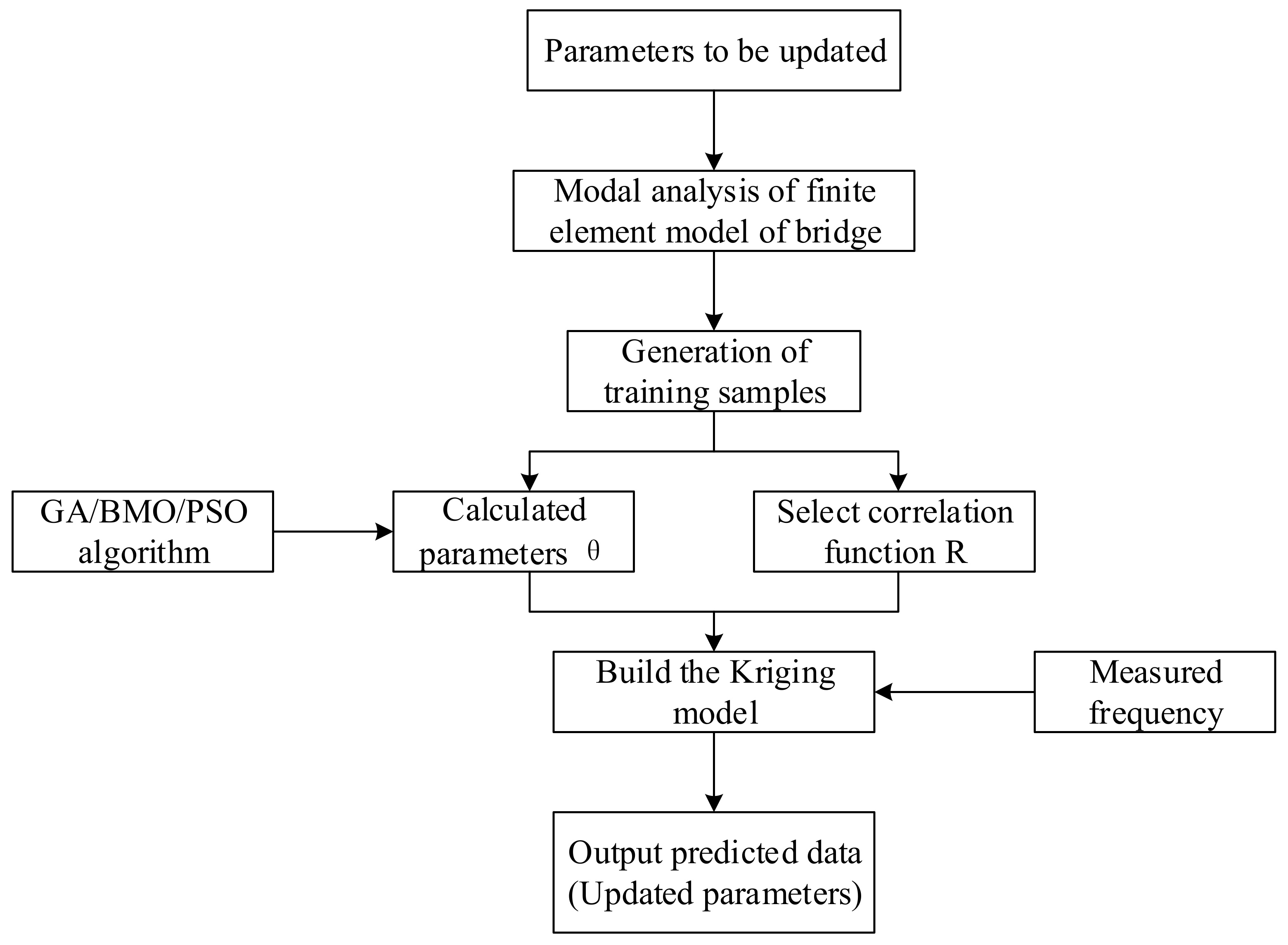
2.1. Kriging Model
- (1)
- Determine the variables to be corrected in the finite element model, and then generate a certain number of samples according to the distribution form of the determined variables.
- (2)
- Substitute the generated samples into the finite element model of the bridge for modal analysis, and extract the modal correlation information corresponding to the variables.
- (3)
- The variables and the corresponding structural mode frequencies are taken as the input and output samples, respectively, and GA, BMO, or PSO is used to optimize the parameters in the correlation function of the Kriging model to complete the establishment of the Kriging model.
- (4)
- Take the frequency of modal test of the bridge as the input, use the Kriging model to predict the structure modal, and extract the variables by finite element model updating.
2.2. Kriging Model Updating Method Based on GA
- (1)
- Code the samples to generate the initial population;
- (2)
- Set the fitness function of the population, which is the inverse of the difference between the modal frequency of the model and the measured field frequency. Then the fitness of the individuals in the population is calculated;
- (3)
- Conduct individual selection, crossover, mutation to generate new progeny population;
- (4)
- Decode the obtained new progeny population and input it into the finite element model to calculate and extract the modal information of the structure;
- (5)
- Obtain the frequency error by comparing the finite element modal frequency with the measured frequency. When the error meets the requirement of accuracy, complete the correction process; if the accuracy cannot meet the requirements, then go back to step (1).
2.3. Kriging Model Updating Method Based on BMO
2.3.1. Monogamy
2.3.2. Polygyny
2.3.3. Promiscuity
2.3.4. Parthenogenesis
2.3.5. Polyandry
2.3.6. Steps
2.4. Kriging Model Updating Method Based on PSO
- (1)
- It is assumed that the total number of particles in the particle swarm is m, which belongs to D-dimensional space. The inertia weight is , the acceleration factor is and , and the maximum flight speed is .
- (2)
- Calculate the fitness value of each particle according to the objective function, compare the current fitness value of each particle with the adaptive value of the optimal individual position, compare the current fitness value of each particle with the fitness value of the global optimal position , and calculate the velocity and position of the particle at the next moment.
- (3)
- Iterative calculation.
- (4)
- Calculate the fitness value of each particle and calculate the optimal position of the individual. Calculate the optimal position of the population and the optimal fitness value of the population, and update the speed and position of the particle.
- (5)
- Determine whether the iteration reaches the maximum number or the convergence threshold. If the iteration reaches the maximum number or the convergence threshold, the optimization will stop. Instead, go back to step 3.
2.5. Latin Hypercube Sampling
- (1)
- Determine the number of samples m to be taken.
- (2)
- Divide the interval of each dimension into m non-overlapping cells with the same probability, and divide the original hypercube into small hypercubes with the number of .
- (3)
- Generation matrix M, whose dimension is . Each column in the matrix M is formed by random arrangement of sequence .
- (4)
- Each row in the matrix M represents a small hypercube to be extracted, and a point is randomly selected from each small hypercube to obtain the required m samples.
3. Finite Element Model Updating for Two Bridges
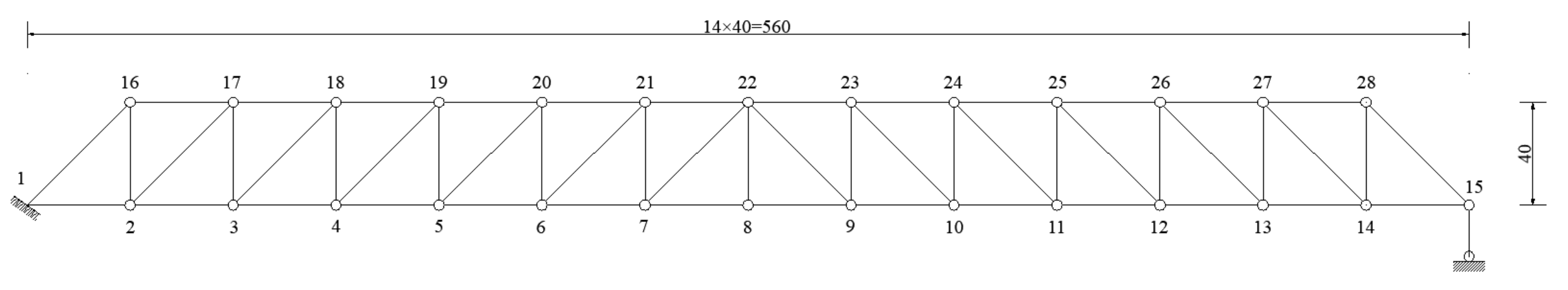
3.1. Verification of Plane Truss
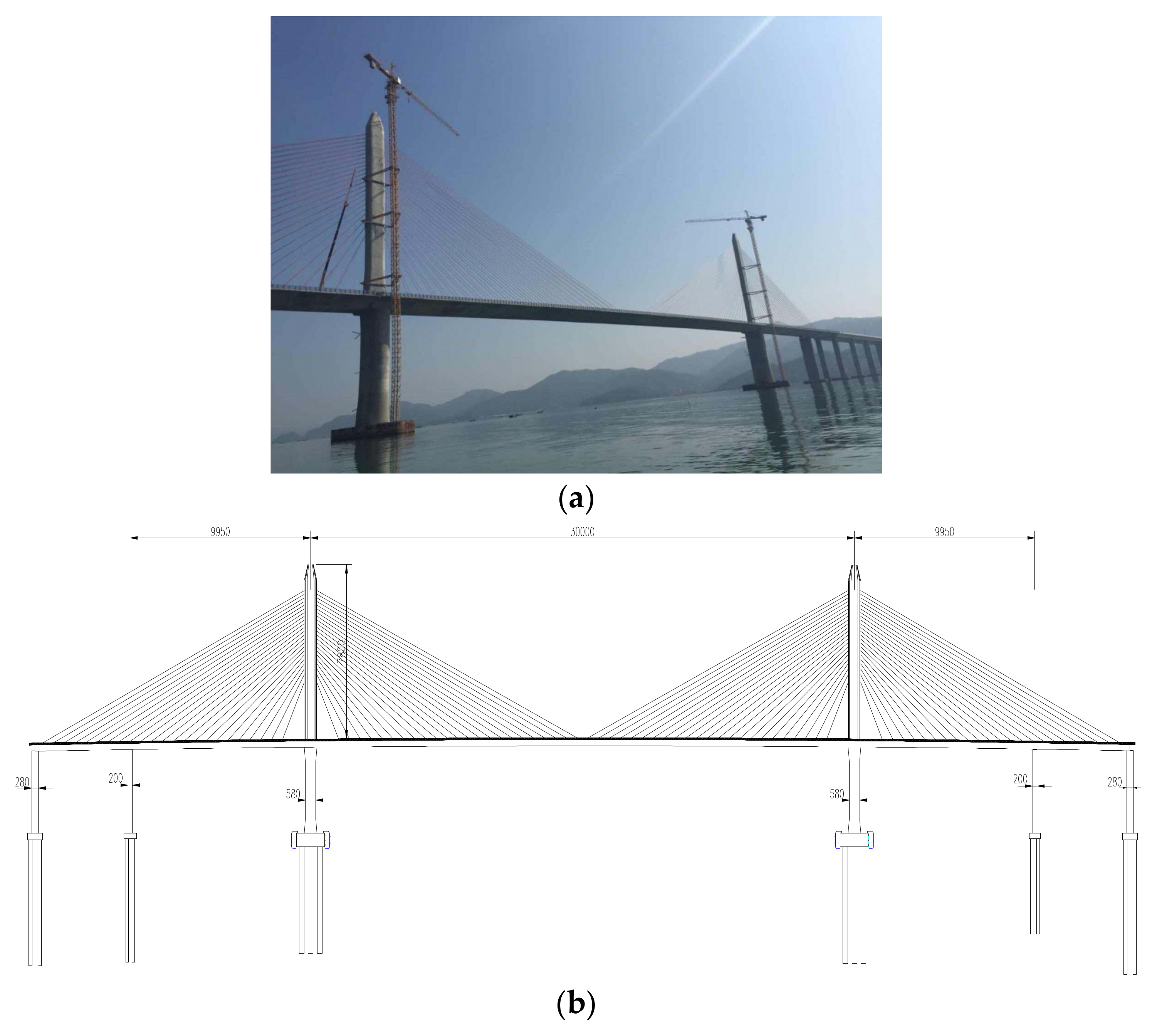
3.2. Finite Element Model Updating for Cable-Stayed Bridge
3.2.1. Description
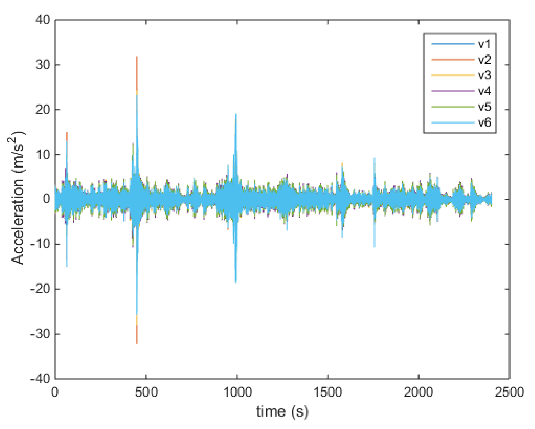
3.2.2. Modal Test
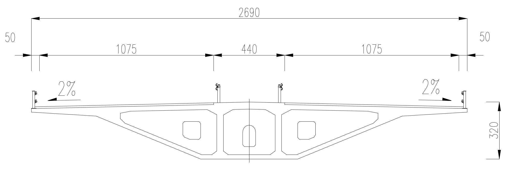
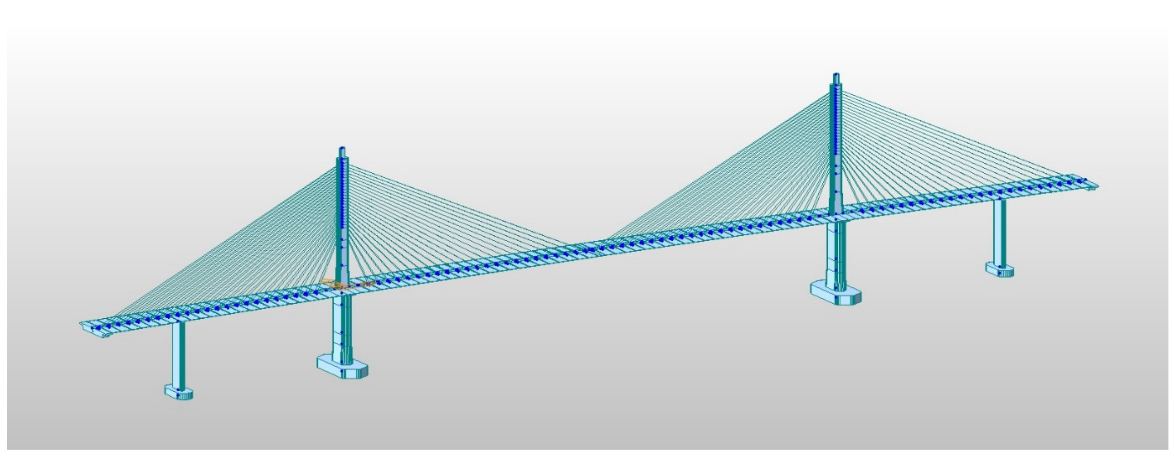
3.2.3. Finite Element Model of Cable-Stayed Bridge
3.2.4. Results
4. Conclusions
Author Contributions
Funding
Institutional Review Board Statement
Informed Consent Statement
Data Availability Statement
Conflicts of Interest
References
- Xu, X.; Huang, Q.; Ren, Y.; Zhao, D.Y.; Yang, J.; Zhang, D.Y. Modeling and separation of thermal effects from cable-stayed bridge response. J. Bridge Eng. 2019, 24, 04019028. [Google Scholar] [CrossRef]
- Xu, X.; Huang, Q.; Ren, Y.; Zhao, D.Y.; Zhang, D.Y.; Sun, H.B. Condition evaluation of suspension bridges for maintenance, repair and rehabilitation: A comprehensive framework. Struct. Infrastruct. Eng. 2019, 15, 555–567. [Google Scholar] [CrossRef]
- Islam, M.M.; Hu, G.; Liu, Q. Online Model Updating and Dynamic Learning Rate-Based Robust Object Tracking. Sensors 2018, 18, 2046. [Google Scholar] [CrossRef] [PubMed] [Green Version]
- Xiong, W.; Cai, C.S.; Kong, B.; Zhang, X.; Tang, P. Bridge Scour Identification and Field Application Based on Ambient Vibration Measurements of Superstructures. J. Mar. Sci. Eng. 2019, 7, 121. [Google Scholar] [CrossRef] [Green Version]
- Kim, S.; Kim, N.; Park, Y.-S.; Jin, S.-S. A Sequential Framework for Improving Identifiability of FE Model Updating Using Static and Dynamic Data. Sensors 2019, 19, 5099. [Google Scholar] [CrossRef] [Green Version]
- Jan, B.; Pawel, H.; Marco, T. SHM system and a FEM model-based force analysis assessment in stay cables. Sensors 2021, 21, 1927. [Google Scholar]
- Alberto, M.B.M.; Luís, M.C.S.; João, H.J.O.N. Optimum design of concrete cable-stayed bridges. Eng. Optimiz. 2016, 48, 772–791. [Google Scholar]
- Farid, G.; Niloofar, M.; Hamed, E.; Ertugrul, T. Bridge Digital Twinning Using an Output-Only Bayesian Model Updating Method and Recorded Seismic Measurements. Sensors 2022, 22, 1278. [Google Scholar]
- Xu, X.; Huang, Q.; Ren, Y.; Zhao, D.Y.; Yang, J. Sensor fault diagnosis for bridge monitoring system using similarity of symmetric responses. Smart Struct. Syst. 2019, 23, 279–293. [Google Scholar]
- Asadollahi, P.; Huang, Y.; Li, J. Bayesian Finite Element Model Updating and Assessment of Cable-Stayed Bridges Using Wireless Sensor Data. Sensors 2018, 18, 3057. [Google Scholar] [CrossRef] [Green Version]
- Cha, P.D.; Tuck-Lee, J.P. Updating structural system parameters using frequency response data. J. Eng. Mech. 2000, 126, 1240–1246. [Google Scholar] [CrossRef]
- Zapico, J.L.; Gonzalez, M.P.; Friswell, M.I.; Taylor, C.A.; Crewe, A.J. Finite element model updating of a small scale bridge. J. Sound Vib. 2003, 268, 993–1012. [Google Scholar] [CrossRef]
- Tran-Ngoc, H.; Khatir, S.; De Roeck, G.; Bui-Tien, T.; Nguyen-Ngoc, L.; Abdel Wahab, M. Model Updating for Nam O Bridge Using Particle Swarm Optimization Algorithm and Genetic Algorithm. Sensors 2018, 18, 4131. [Google Scholar] [CrossRef] [Green Version]
- Kirkpatrick, S.; Gelatt, C.D.; Vecchi, M.P. Optimization by simulated annealing. Science 1983, 220, 671–680. [Google Scholar] [CrossRef]
- Levin, R.I.; Lieven, N.A.J. Dynamic finite element model updating using simulated annealing and genetic algorithms. Mech. Syst. Signal Process. 1998, 12, 91–120. [Google Scholar] [CrossRef] [Green Version]
- Astroza, R.; Nguyen, L.T.; Nestorović, T. Finite element model updating using simulated annealing hybridized with unscented Kalman filter. Comput. Struct. 2016, 177, 176–191. [Google Scholar] [CrossRef]
- Guo, J.; Yuan, W.; Dang, X.; Alam, M.S. Cable force optimization of a curved cable-stayed bridge with combined simulated annealing method and cubic B-Spline interpolation curves. Eng. Struct. 2019, 201, 109813. [Google Scholar] [CrossRef]
- He, S.; Ng, C.T. A probabilistic approach for quantitative identification of multiple delaminations in laminated composite beams using guided waves. Eng. Struct. 2016, 127, 602–614. [Google Scholar] [CrossRef] [Green Version]
- Behmanesh, I.; Moaveni, B. Probabilistic identification of simulated damage on the Dowling Hall footbridge through Bayesian finite element model updating. Struct. Control Health Monit. 2015, 22, 463–483. [Google Scholar] [CrossRef]
- Guo, N.; Yang, Z.; Wang, L.; Bian, X. A updating method using strain frequency response function with emphasis on local structure. Mech. Syst. Signal Process. 2019, 115, 637–656. [Google Scholar] [CrossRef]
- Shabbir, F.; Omenzetter, P. Model updating using genetic algorithms with sequential niche technique. Eng. Struct. 2016, 120, 166–182. [Google Scholar] [CrossRef]
- Li, B.; Yang, X.; Xuan, H. A hybrid simulated annealing heuristic for multistage heterogeneous fleet scheduling with fleet sizing decisions. J. Adv. Transp. 2019, 5364201. [Google Scholar] [CrossRef]
- Katahira, K. The statistical structures of reinforcement learning with asymmetric value updates. J. Math. Psychol. 2018, 87, 31–45. [Google Scholar] [CrossRef]
- Bartilson, D.T.; Jang, J.; Smyth, A.W. Finite element model updating using objective-consistent sensitivity-based parameter clustering and Bayesian regularization. Mech. Syst. Signal Process. 2019, 114, 328–345. [Google Scholar] [CrossRef]
- Zhu, J.J.; Huang, M.; Lu, Z.R. Bird mating optimizer for structural damage detection using a hybrid objective function. Swarm Evol. Comput. 2017, 35, 41–52. [Google Scholar] [CrossRef]
- Qin, S.; Zhang, Y.; Zhou, Y.-L.; Kang, J. Dynamic Model Updating for Bridge Structures Using the Kriging Model and PSO Algorithm Ensemble with Higher Vibration Modes. Sensors 2018, 18, 1879. [Google Scholar] [CrossRef] [Green Version]
- Wu, J.; Yan, Q.; Huang, S.; Zou, C.; Zhong, J.; Wang, W.W. Finite Element Model Updating in Bridge Structures Using Kriging Model and Latin Hypercube Sampling Method. Adv. Civ. Eng. 2018, 2018, 8980756. [Google Scholar] [CrossRef]
- Wang, Z.; Shafieezadeh, A. Real-time high-fidelity reliability updating with equality information using adaptive Kriging. Reliab. Eng. Syst. Saf. 2020, 195, 106735. [Google Scholar] [CrossRef]
- Krige, D.G. A Statistical Approach to Some Mine Valuation and Allied Problems on the Witwatersrand. Master’s Thesis, Faculty of Engineering, University of the Witwatersrand, Johannesburg, South Africa, 1951. [Google Scholar]
- Lophaven, S.N.; Nielsen, H.B.; Søndergaard, J. DACE—A Matlab Kriging Toolbox; IMM-TR-2002-12; Technical University of Denmark: Lyngby, Denmark, 2002; pp. 1–28. [Google Scholar]
- McKay, M.D.; Beckman, R.J.; Conover, W.J. A comparison of three methods for selecting values of input variables in the analysis of output from a computer code. Technometrics 2000, 42, 55–61. [Google Scholar] [CrossRef]
- Yan, G.R.; Duan, Z.D.; Ou, J.P. Application of genetic algorithm on structural finite element model updating. J. Harbin Inst. Technol. 2007, 39, 181–186. (In Chinese) [Google Scholar]


| Order | Measured | Ref. [32] | GA | BMO | PSO | ||||
|---|---|---|---|---|---|---|---|---|---|
| Modal Frequency | Error | Modal Frequency | Error | Modal Frequency | Error | Modal Frequency | Error | ||
| 1 | 8.79 | 8.83 | −0.55% | 8.79 | 0.00% | 8.76 | 0.34% | 8.75 | −0.46% |
| 2 | 29.60 | 30.18 | −1.48% | 29.78 | −0.60% | 29.98 | 1.28% | 29.78 | −0.60% |
| 3 | 43.39 | 41.65 | 2.23% | 42.66 | 1.69% | 43.14 | −0.58% | 42.92 | 1.08% |
| 4 | 59.10 | 59.62 | −0.24% | 59.55 | −0.75% | 59.77 | −1.13% | 59.19 | −0.15% |
| 5 | 90.62 | 91.34 | −0.40% | 91.09 | −0.52% | 90.75 | 0.14% | 90.85 | 0.25% |
| 6 | 119.81 | 120.84 | −0.11% | 120.86 | −0.88% | 119.95 | 0.12% | 119.88 | 0.06% |
| Order | Measured | Finite Element Model | Error (%) | Modal |
|---|---|---|---|---|
| 1 | 0.4639 | 0.4582 | 1.23 | Vertical bending |
| 2 | 0.6507 | 0.5981 | 8.08 | Antisymmetric vertical bending |
| 3 | 1.1960 | 1.0517 | 12.07 | Vertical bending |
| 4 | - | 1.5123 | - | Vertical bending |
| 5 | 1.9814 | 1.9806 | 0.04 | Vertical bending |
| 6 | 2.6415 | 2.6222 | 0.73 | Vertical bending |
| Order | Measured Natural Frequency | GA Natural Frequency | BMO Natural Frequency | PSO Natural Frequency |
|---|---|---|---|---|
| 1 | 0.4639 | 0.4595 | 0.4611 | 0.4622 |
| 2 | 0.6507 | 0.6351 | 0.6375 | 0.6398 |
| 3 | 1.1960 | 1.1462 | 1.1453 | 1.1538 |
| 5 | 1.9814 | 1.9785 | 1.9825 | 1.9811 |
| 6 | 2.6415 | 2.6209 | 2.6235 | 2.6285 |
| Parameters | Not Updating | GA | BMO | PSO | Coefficient of Variation |
|---|---|---|---|---|---|
| Ec1/GPa | 35.50 | 35.08 | 35.21 | 35.68 | 10% |
| γc1/(N/m3) | 26,000 | 26,121 | 25,874 | 26,225 | 10% |
| Ec2/GPa | 36.00 | 35.21 | 35.87 | 36.33 | 10% |
| γc2/(N/m3) | 26,000 | 25,854 | 26,172 | 26,228 | 10% |
| GA | BMO | PSO |
|---|---|---|
| 0.5 | 1.1 | 1.5 |
| Order | Not Updating | GA | BMO | PSO |
|---|---|---|---|---|
| 1 | 0.9325 | 0.9083 | 0.9245 | 0.9588 |
| 2 | 0.9182 | 0.9192 | 0.9199 | 0.9215 |
| 3 | 0.9923 | 0.9921 | 0.9925 | 0.9933 |
| 5 | 0.9322 | 0.9304 | 0.9338 | 0.9358 |
| 6 | 0.9159 | 0.9158 | 0.9164 | 0.9172 |
| Not Updating | GA | BMO | PSO |
|---|---|---|---|
| 0.1788 | 0.0506 | 0.0475 | 0.0394 |
Publisher’s Note: MDPI stays neutral with regard to jurisdictional claims in published maps and institutional affiliations. |
© 2022 by the authors. Licensee MDPI, Basel, Switzerland. This article is an open access article distributed under the terms and conditions of the Creative Commons Attribution (CC BY) license (https://creativecommons.org/licenses/by/4.0/).
Share and Cite
Wu, J.; Cheng, F.; Zou, C.; Zhang, R.; Li, C.; Huang, S.; Zhou, Y. Swarm Intelligent Optimization Conjunction with Kriging Model for Bridge Structure Finite Element Model Updating. Buildings 2022, 12, 504. https://doi.org/10.3390/buildings12050504
Wu J, Cheng F, Zou C, Zhang R, Li C, Huang S, Zhou Y. Swarm Intelligent Optimization Conjunction with Kriging Model for Bridge Structure Finite Element Model Updating. Buildings. 2022; 12(5):504. https://doi.org/10.3390/buildings12050504
Chicago/Turabian StyleWu, Jie, Fan Cheng, Chao Zou, Rongtang Zhang, Cong Li, Shiping Huang, and Yu Zhou. 2022. "Swarm Intelligent Optimization Conjunction with Kriging Model for Bridge Structure Finite Element Model Updating" Buildings 12, no. 5: 504. https://doi.org/10.3390/buildings12050504
APA StyleWu, J., Cheng, F., Zou, C., Zhang, R., Li, C., Huang, S., & Zhou, Y. (2022). Swarm Intelligent Optimization Conjunction with Kriging Model for Bridge Structure Finite Element Model Updating. Buildings, 12(5), 504. https://doi.org/10.3390/buildings12050504