Abstract
The rapid development of public buildings has greatly increased the country’s energy consumption and carbon emissions. Excessive carbon emissions contribute to global warming. This paper aims to measure the carbon emissions in the operation of public buildings, and to identify the multiple influencing factors of carbon emissions in operational public buildings. First, the spatial and temporal variation characteristics of carbon emissions from public buildings in 30 provinces of China from 2008–2019 are analyzed. Second, a green building index is constructed, and the STIRPAT (Stochastic Impacts by Regression on Population, Affluence, and Technology) model is utilized to explore the relationship between each influencing factor and carbon emissions, using spatial and temporal geographically weighted regression analysis. The results show that the effects of population, urbanization rate, GDP per capita, green building index, and industrial structure on carbon emissions from public buildings all show spatial correlation and differences. There are east-west differences in the operational carbon emissions of public buildings in China’s provinces. Cluster evolution shows a spatially increasing trend from west to east. To some extent, policymakers can develop appropriate policies for different provinces through the findings.
1. Introduction
Climate change has become one of the most important globally recognized issues. Reducing CO2 emissions helps mitigate climate change, and carbon emission and environmental protection issues have aroused the attention of various countries. Many countries have begun to measure carbon emissions and take action to reduce them [1,2]. Recently, the Chinese government announced that it strives to achieve carbon peaking by 2030, and carbon neutrality by 2060. More detailed plans have also been specified to reach this goal. By 2030, carbon dioxide emissions per unit of GDP will drop 65% compared to 2005, the proportion of non-fossil energy consumption will reach about 25%, and the total installed capacity of solar and wind power generation will reach more than 1.2 billion kilowatts. The Ministry of Ecology and Environment has proposed that during the 14th and 15th Five-Year Plan periods, China will carry out CO2 emission peaking actions and specify the peaking targets and action plans for localities and industries. China’s total construction carbon emissions were 4.93 billion tons in 2018, accounting for 51% of the national carbon emissions. Carbon emissions from the production phase of building materials account for 28% of the total national carbon emissions, the construction phase accounts for 1%, and the building operation phase is 22% [3].
According to the data in 2018, the existing stock of public buildings in China’s urban and rural areas is 12.8 billion square meters, accounting for 21.3% of the total civil construction area. From the annual data, the energy consumption for the construction of public buildings accounted for 44% of the total building construction energy consumption in 2018, and the total energy consumption for the operation of public buildings excluding northern heating accounted for 33% of the total building operation energy consumption [4].
In 2015, the energy consumption of public buildings in China was 34.1 billion tons of standard coal equivalent, accounting for about 40% of the total energy consumption of civil buildings. However, the public building area accounted for only 18% of the total area of civil buildings. Furthermore, a study showed that the energy intensity of public buildings in China was four times that of residential buildings from 2000 to 2015. Public buildings are important places for human activities, and their construction, operation, renewal, and demolition processes all generate significant energy consumption. Therefore, the CO2 emissions of public buildings in China have attracted more attention [5].
Green buildings play a very important role in reducing carbon emissions. Wu et al. (2017) [6] found that with commercial buildings in China, green buildings are lower in carbon emissions than non-green buildings, in the operational phase. The Chinese government proposed the Green Building Creation Initiative in 2020, which aims to reach 70% of the green building area in new urban buildings in that year by 2022. The effect of green building on carbon reduction in the building sector and its spatial evolution is the focus of this study.
2. Literature Review
2.1. Spatiotemporal Analysis of Carbon Emission
Spatiotemporal analysis is a method that considers both temporal data and spatial position, and is mainly used to solve how coherent entities change over time. Scholars have performed many researches with different methods to study the spatiotemporal analysis of carbon emission and its influencing factors in different fields. For example, Chen et al. (2021) analyzed the temporal and spatial characteristics of industrial carbon emissions in four regions of Guangdong province from 2005 to 2015, and concluded that industrial carbon emissions have a trend of eastward expansion [7]. The spatial dynamic analysis model (SDDM) was used to study the impact of different technological progress factors on carbon emissions [8]. Cui et al. (2021) explored spatiotemporal dynamic evolution of carbon emission intensity and per capita carbon emissions from planting industry in 31 provinces in China across 20 years. The spatial inequality is measured by Theil index and its contribution rate [9]. Wang et al. (2020) employed the standard deviation ellipse method and tapio decoupling method to reveal the spatiotemporal characteristics of the relationship between carbon emissions from transportation industry and economic growth [10]. Hu et al. (2020) studied the spatial and temporal evolution relationship between economic growth and carbon emissions in Belt and Road countries [11]. Han et al. (2021) revealed the spatiotemporal characteristics of carbon intensity of 20 industries by extending the spatial weight matrix and spatial dubin model [12]. Falahatkar et al. (2020) quantified the relationship between carbon dioxide emission and urban form in 15 Iranian cities, and believed that carbon dioxide emission level was positively correlated with urban area growth and urban complexity increase [13]. Some scholars have studied the carbon emission spatiotemporal effect in the construction industry. Bai et al. (2021) estimated the building inventory and carbon emissions embodied by buildings in 31 provinces of China from 1997 to 2016, and proposed a spatiotemporal decomposition model to identify driving forces [14]. To sum up, in the construction industry, there are few spatial analyses on carbon emissions during the operation of public buildings.
2.2. Influencing Factors of Buildings Carbon Emission
The extraction of raw materials, on-site construction activities, and building operations produced the majority of carbon emissions of the construction sector [4]. Hard coal and its derivatives were the largest carbon dioxide emitters in China’s construction industry [15]. In view of the significant impact of the construction industry, prior studies have been carried out to investigate influencing factors in order to develop mitigation strategies. For example, Lu et al. (2016) have analyzed the influencing factors of carbon emissions from construction activities in China, including energy intensity, energy structure, unit cost, level of construction automation, and machine efficiency [16]. Similarly, Zhang, Yan et al. (2019) stated that building scale, building structure type, and production efficiency of material are the three main driving factors [4]. Wu, shen et al. (2019) used the STIRPAT model and found that the impact of population size, per capita GDP, energy intensity, and industrial structure on carbon emissions were heterogeneous among regions [17]. Mostafavi, Tahsildoost et al. concluded that strengthening the design parameters of envelope structure, optimizing the layout, and utilizing natural ventilation are conducive to reducing energy consumption of high-rises [18]. Tan, Lai, Gu, Zeng, & Li constructed a carbon emission prediction model including population, urbanization rate, and urban building area [19]. Wang et al. explored the driving forces of energy-related CO2 emissions in the construction industry by implementing the comprehensive decomposition method, and finally found that technological progress of industrial output was the leading factor that suppressed CO2 emissions [20]. Huang et al. propounded increased energy efficiency design for new buildings and energy-saving retrofit for existing buildings to carbon emission [21].
2.3. Research Gap
Based on a critical review of relevant studies, as well as substantive surveys and interviews with Chinese building industry professionals, we conclude that the spatial and temporal effects of carbon emissions from public buildings still require further research. Because using the STIRPAT model to decompose influence factor is more comprehensive, it is still worthwhile to use this model to study the factors that drive the carbon emission of operational public buildings.
3. Data Source and Methodologies
3.1. Study Area
China has 34 provincial districts. Four provincial districts (Tibet, Macao, Hong Kong, and Taiwan) are excluded due to data unavailability, so this study selected a total of 30 provincial districts. The study divided 30 provincial districts into four regions (East region, Central region, West region, and Northeast region) according to the National Bureau of Statistics (Table 1).

Table 1.
Four regions and their provincial districts.
3.2. Data Source
The data of green buildings from 2008 to 2016 and 2018 to 2019 are obtained from the Chinese Green Building Evaluation Label Network. Green building data in 2017 are obtained through compilation of public information of green building projects on the website of provincial Construction Department. The remaining indicators are from China Energy Statistical Yearbook and China Statistical Yearbook for 2009–2020. The map data comes from the National Geomatics Center of China.
3.3. Methodology
3.3.1. Hot Spot Analysis
statistic is used to analyze the spatial aggregation degree of carbon emissions during the operation of provincial public buildings, as shown in Equation (1).
is the attribute value of the unit , and is the carbon emission in th province public buildings during its operation; is the spatial weight matrix.
is standardized by Equation (2) and the result is . The larger the value is, the higher the spatial clustering in the region, indicating that it belongs to the hot spot area; the smaller it is, the lower the spatial clustering in the region, indicating it belongs to the cold spot area.
where , are the expectation and variance of , respectively.
3.3.2. Geographically and Temporally Weighted Regression Model
The geographically and temporally weighted regression (GTWR) model is a deepening of the geographically weighted regression model, as shown in Equation (3). By using regional panel data for spatial regression, the temporal attributes are linked to the spatial attributes in the GTWR model, which better reflects the spatial and temporal change information of the study area, and makes the estimation results more effective.
where is the dependent variable of sample , is the th independent variable at the sample point , , are the latitude and longitude coordinates of the center of gravity, respectively, are the spatial and temporal coordinates of the th sample, is the regression coefficient on the th independent variable at the th sample point, is the space-time intercept of the th sample point, and is the residual term.
3.3.3. Model Specification
Enrlich and Holdren first put forward the classic IPAT model in the early 1970s, which stipulates the influence of external factors on the environment. External factors include population size (P), affluency (A), and technology (T). The IPAT model was improved and transformed into the nonlinear random STIRPAT model, which is often used to analyze influencing factors of carbon emissions in different industries [22]. For example, Ma et al. surveyed the driving factors of carbon dioxide emission from public buildings in a country [23,24]; Yang and Jia explored the spatial effects of technology progress channels on CO2 emissions for the agricultural, industrial, construction, transportation, and wholesale sectors [25]. The STIRPAT model is expressed as Equation (4):
where denotes the regional unit. , , and represent the impacts on the environment owing to population, affluence (per capita GDP), and technology factors in region , respectively. Constant a represents the scale of the model. Meanwhile, , , and are the estimated coefficients of population, affluence (per capita GDP), and technology, respectively. is the random error term. We take the logarithm of the STIRPAT model, obtaining the following Equation (5):
The STIRPAT equation allows the addition of plenty of relevant variables, and the transformation of the model into an extended version, as long as the dimensionality of these variables is reasonable [26,27].
In order to deeply explore the mechanism of carbon emission of public buildings, considering green buildings’ specific characteristics, and looking for supporting references from a great deal of relevant previous studies, this study developed an extended version of the STIRPAT model using several meaningful variables retrieved from the population, affluence, and technology levels, respectively. The extended STIRPAT model is expressed in Equation (6):
where refers to the carbon emission in the public building sector in province over time . represents spatial coordinates of province (i = 1, 2, 3, ..., 30). ( = 1, 2, 3, 4, 5) denotes the th regression coefficient in the th province. The meaning and units of the variables are shown in Table 2.
Table 2.
Declaration of the model variables.
3.3.4. Index Calculation
- Calculation methods of CO2 emission
The operational energy consumption of public buildings includes heating, air conditioning, ventilation, lighting, elevators, cooking, domestic hot water, office electrical equipment, and comprehensive service equipment and facilities. Corresponding energy types include electricity, gas (natural gas, gas, and LPG), fuel oil (diesel), and coal combustion. This study uses a macro model for measuring carbon emissions from buildings based on energy balance sheets.
This paper mainly studies the operational stage of carbon emissions in public buildings. Because China’s energy statistics yearbook does not provide building energy consumption directly [33], we need to select the energy consumption as public buildings’ operational consumption. The specific accounting boundaries are shown in Table 3.
Table 3.
Specific accounting boundary of public building.
This study mainly measures carbon emissions during the use of public buildings. Carbon emission in Chinese public buildings is measured by the end-use consumption of energy in each region in the China Energy Statistics Yearbook. The industries involved in public buildings are Transport, Storage and Post, Wholesale and Retail Trades, Hotels and Catering Services, and Other.
Energy type measurement includes coal, electricity, natural gas, LPG, and thermal power. Oil is not counted because it is mostly used in public buildings for transportation involving cars, and is not counted as energy consumption inside buildings for the time being. To obtain more meaningful and comprehensive results, we included three types of energy sources, such as coal, natural gas, and liquefied petroleum gas. According to the calculation method provided by IPCC (Equation (7)), coal, electricity, and heat consumed in the operation of public buildings are taken as the sources of carbon emissions.
where denotes the total carbon emissions from public building operation in each province, refers to carbon emission of the consumption of fossil energy in the province, and and represent the carbon emissions from the secondary energy consumption of electricity and heat in the province. denotes the consumption of fossil energy in the province; refers to the oxidation rate of the fossil energy in the province ; represents the average low-level calorific value of fossil energy in province ; denotes the carbon emission factor of fossil energy in province ; factor refers to the ratio of CO2 molecules to carbon atoms by weight; carbon emissions can be converted into CO2 emissions by multiplying by this coefficient, and denote the electricity consumption and heat consumption in province , respectively, and denote the carbon emission factor of electricity and heat consumption in province .
The carbon emissions generated during the use of public buildings are estimated by referring to the low level calorific value, carbon emission factor, and carbon oxidation rate provided by IPCC.
Since the carbon emission factor of coal is not directly provided in IPCC, coal is considered as raw coal for calculation. The carbon emission factor of coal is 25.8 TC/TJ, the low calorific value is 20.908 GJ/T, and the carbon oxidation rate is 0.899. LNG is converted to natural gas volume for calculation, depending on its density as 0.42~0.46 g/cm3.
The average CO2 emission factors (kg-CO2/kWh) of the national regional power grids in 2011 and 2012, as queried by the NDRC and the Guidelines for Provincial Greenhouse Gas Inventories, are shown in Table 4.
Table 4.
Electricity carbon emission factors.
Electricity carbon emission coefficients obtained based on public data query are generally measured by the government or relevant departments in a unified manner, which is easily accessible, and their data source is authoritative. However, the data are not published annually, which is not conducive to the measurement of time series of building carbon emission data. The average value of these two years was used in this study. Inner Mongolia power emission factor is taken as the average value of 0.8442 in the east and west. Table 5 shows Coefficient Thermal CO2 emission [34].
Table 5.
Coefficient Thermal CO2 emission (tCO2/MWh).
- 2.
- Index of green building
Green buildings in China are classified as one-star, two-star, and three-star. Three stars are the highest level of green building. The index of green building is calculated through Equation (8).
where , , denote the number of one-star, two-star and three-star public green buildings in China, respectively.
- 3.
- Industrial Structure
We use the percentage of added value of the tertiary industry to GDP to describe industrial structure [35].
4. Empirical Results
4.1. Spatial Distribution of Carbon Emission in Different Areas
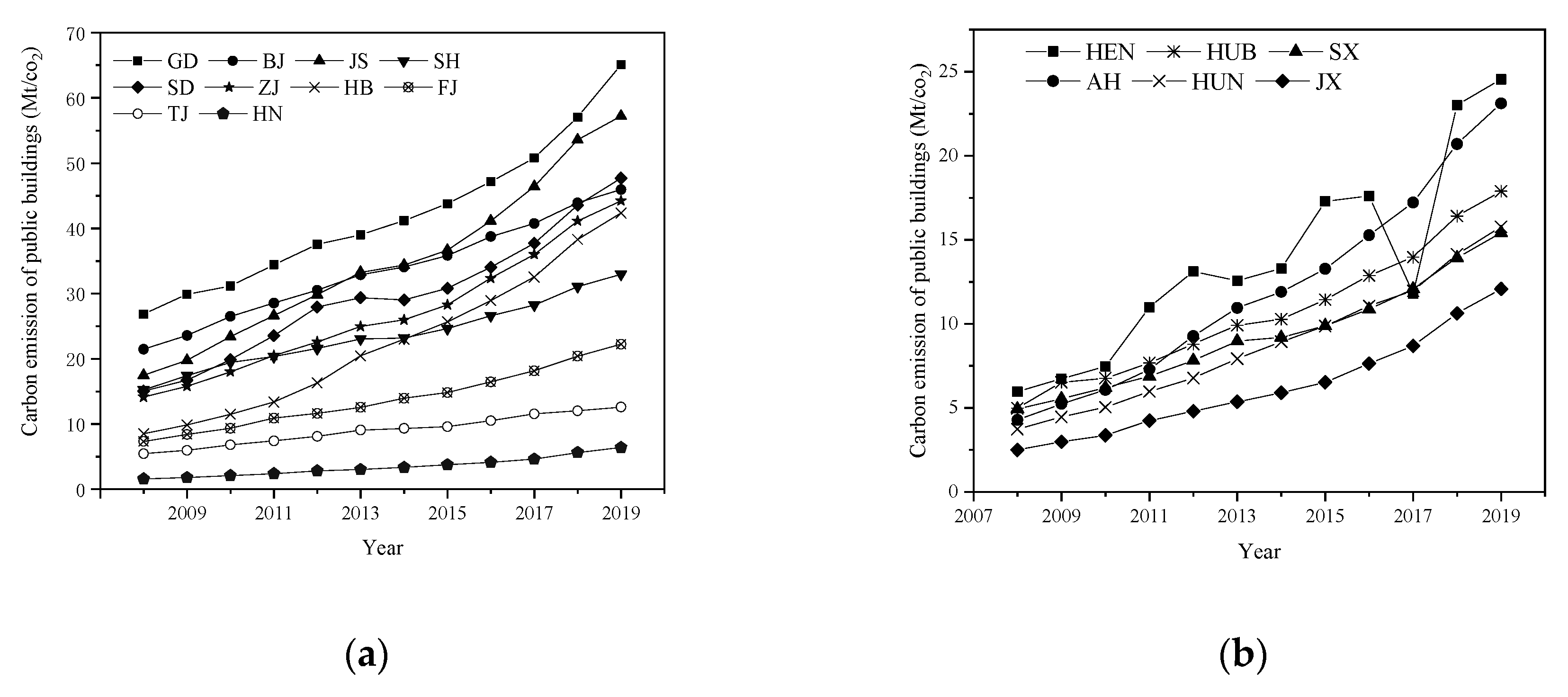
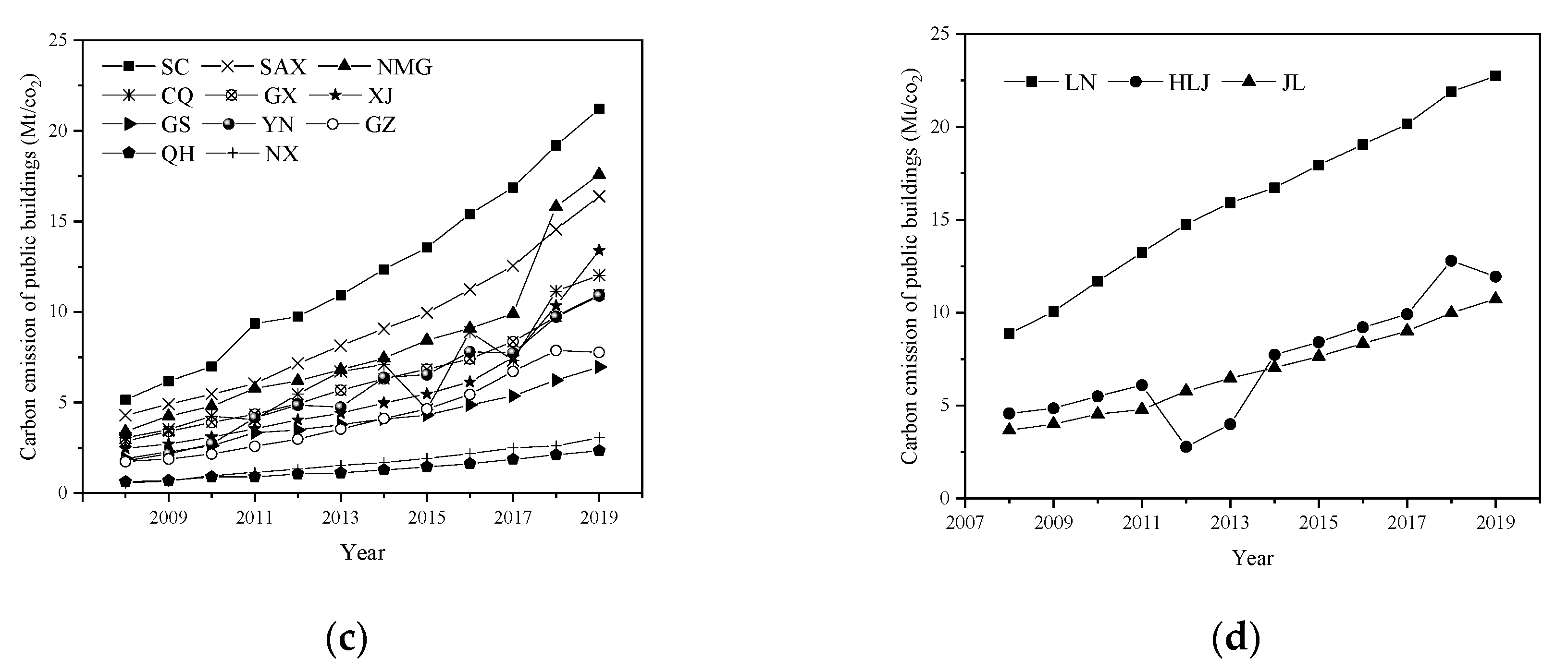
The regional energy balance of the China Energy Statistics Yearbook for 2009–2020 was used to estimate the carbon emissions from the operation of public buildings in each province of the country using end-use energy consumption. The specific measurement results, in accordance with the previously stated zoning, are shown in Figure 1.


Figure 1.
Carbon emission of public buildings in China among provinces during 2008 to 2019: (a) Eastern Region; (b) Central Region; (c) Western Region; (d) Northeast Region. GD—Guangdong, BJ—Beijing, JS—Jiangsu, SH—Shanghai, SD—Shandong, ZJ—Zhejiang, HB—Hebei, FJ—Fujian, TJ—Tianjin, HN—Hainan, HEN—Henan, HUB—Hubei, SX—Shanxi, AH—Anhui, HUN—Hunan, JX—Jiangxi, SC—Sichuan, SAX—Shaanxi, NMG—Inner Mongolia, CQ—Chongqing, GX—Guangxi, XJ—Xinjiang, GS-Gansu, GZ—Guizhou, QH—Qinghai, NX—Ningxia, LN—Liaoning, HLJ—Heilongjiang, JL—Jilin.
In general, the eastern region has more carbon emissions than the central, western, and northeastern regions. The top three provinces generating carbon emissions from public buildings from 2008–2018 were Guangdong, Jiangsu, and Beijing. In 2019, Shandong surpassed Beijing among the top three.
Among the eastern regions, Guangdong Province has the most carbon emissions from public buildings and Hainan Province has the least. All provinces show an increasing trend year by year. Jiangsu Province and Hebei Province have a faster growth rate. In the central region, Henan Province is has the highest carbon emissions, except for 2017, and Jiangxi Province has the lowest carbon emissions. Other regions are steadily increasing, however, not as much as the vast majority of the eastern region’s emissions.
Among the western regions, Sichuan Province consistently has the highest carbon emissions from public buildings, and Qinghai Province steadily has the lowest. Chongqing fluctuated more, with carbon emissions decreasing in 2015 and 2017. The growth rate is larger in Inner Mongolia and Xinjiang. Carbon emissions in Inner Mongolia province were always lower than Shaanxi province between 2008 and 2017, and exceeded Shaanxi province after 2018. Xinjiang Province surpassed Chongqing, Yunnan Province, and Guangxi Province in 2018.
In Northeast China, Liaoning Province has the highest carbon emissions from public buildings. Carbon emissions from public buildings in Heilongjiang Province were higher than those in Jilin Province, except in 2012 and 2013.
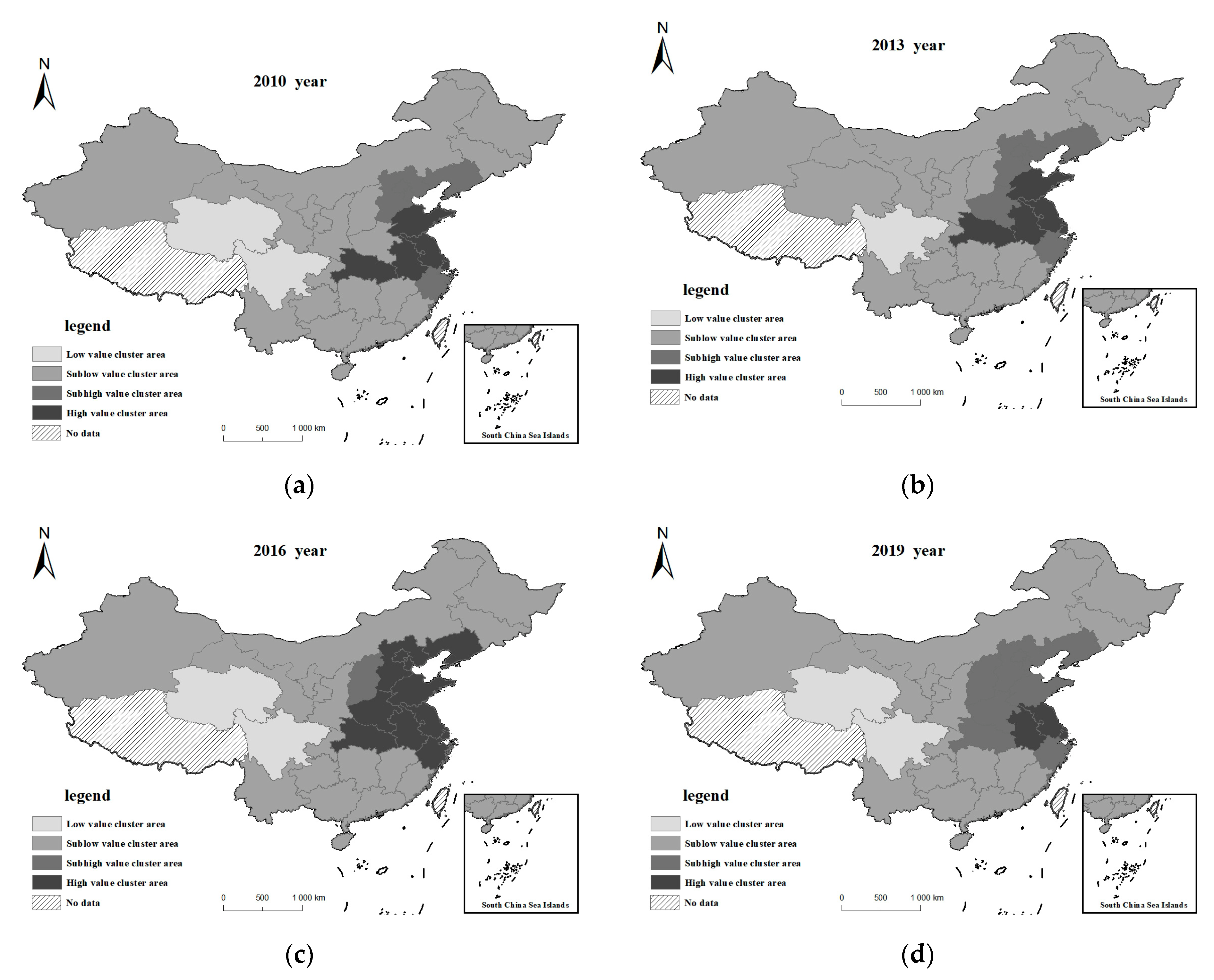
4.2. Hot Spot Analysis of Carbon Emissions from Public Building Operations
Hot spot analysis can reflect the spatial aggregation effect of carbon emissions from public buildings. The variation of the aggregation can be seen by plotting the hot spot and cold spot areas in different years. The natural interruption point grading method was used to classify the values of each year, calculated by Equations (1) and (2) into high, subhigh, sublow, and low value cluster areas in order of largest to smallest. The study area of this research is in the years 2008–2019, and the clustering results of 2010, 2013, 2016, and 2019 are drawn equally spaced for analysis, as shown in Figure 2.
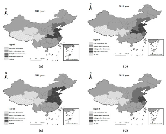
Figure 2.
Spatial agglomeration pattern of public building carbon emissions in China from 2008 to 2019: (a) Spatial agglomeration pattern of public building carbon emissions in China in 2010; (b) Spatial agglomeration pattern of public building carbon emissions in China in 2013; (c) Spatial agglomeration pattern of public building carbon emissions in China in 2016; (d) Spatial agglomeration pattern of public building carbon emissions in China in 2019.
From Figure 2, it can be seen that evolution of provincial carbon emission clustering in China shows a spatially increasing trend from west to east. Overall, the high-value clustering areas are mainly concentrated in Zhejiang, Jiangsu, Anhui, and Shanghai. The low-value clustering areas are mainly concentrated in Qinghai and Sichuan. In 2016, the number of provinces with high-value clustering areas increased, then decreased in 2019. Over time, the high value cluster areas first expanded and then contracted.
4.3. Spatial Effects of the Influencing Factors of Public Buildings Carbon Emissions
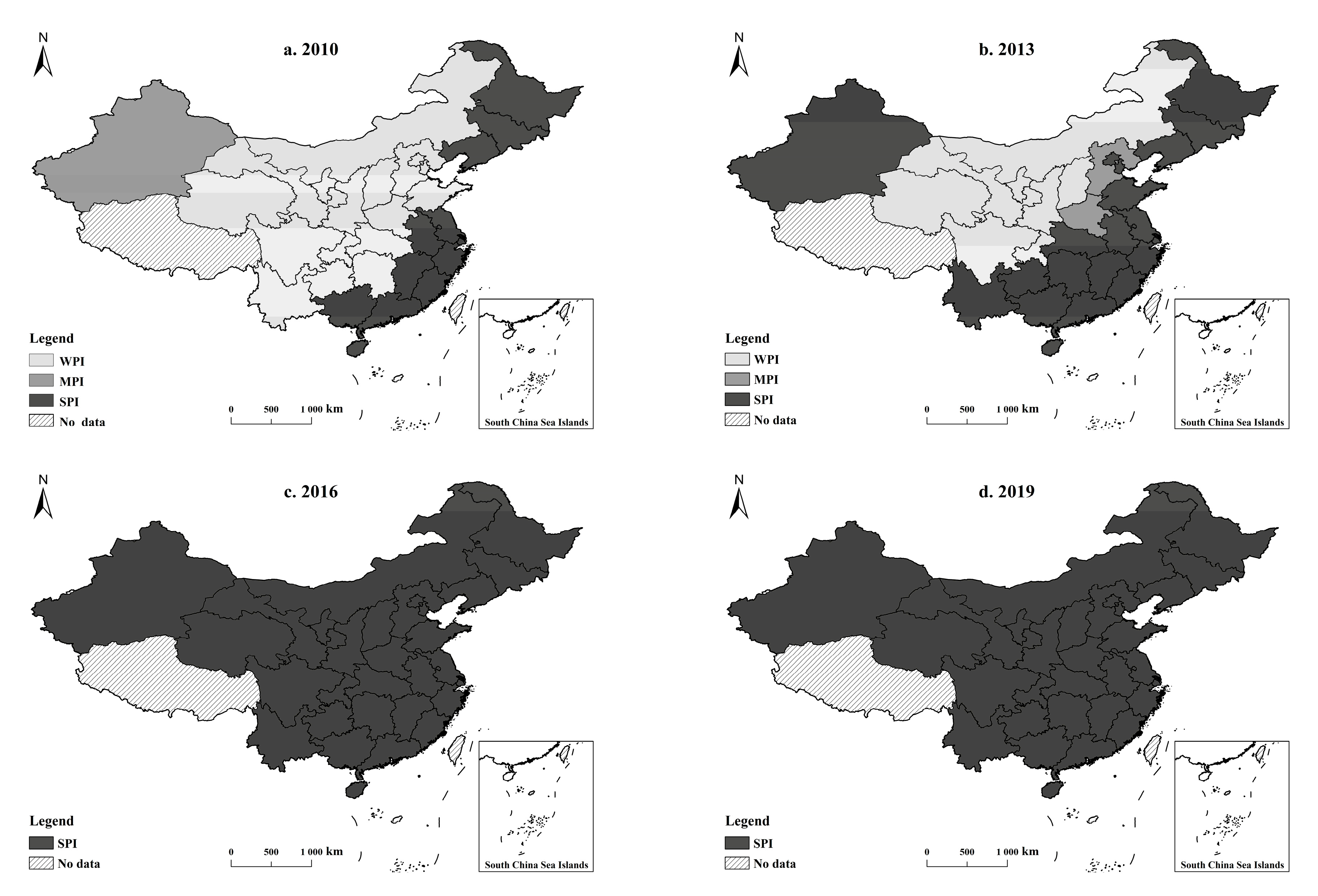
Carbon emissions from public building operations are the dependent variable; population, urbanization rate, industrial structure, GDP per capita, and green index are the explanatory variables in the STIRPAT model; the time range is 2008–2019; and the X and Y coordinates are the geographic coordinates of each province. With these factors, the runs can be entered into the spatio-temporal geographically weighted model to obtain the influence size of the five explanatory variables. In order to unify the comparison of influence size, the influence size values are arranged in descending order and divided by equal spacing, and the positive and negative influence are divided into six levels. Positive influence includes weak (WPI), medium (MPI), and strong positive influence (SPI), which indicates that the influence factor positively contributes to the carbon emission of public building operation; the negative influence includes weak (WNI), medium (MNI), and strong negative influence (SNI), which indicates that the influence factor negatively inhibits the carbon emission of public building operation [36]. Due to the number of years, this study selected 2010, 2013, 2016, and 2019 for spatial presentation and analysis. The GTWR model was run with an adjusted R2 of 0.956 and an AICc of 199.253, indicating a better model effect.
Based on the regression results of the GTWR model, the spatial and temporal variability of the five influencing factors of carbon emissions of public buildings is analyzed one by one.
- Spatial and temporal variation in the effect of population on carbon emissions
Population is a positive influence on the carbon emissions of public buildings in each province. The maximum value of the population regression coefficient is 8.135 and the minimum value is 0.082, which can be divided into WPI, MPI, and SPI according to the influence level. From the results, the provinces with the highest impact are Shanghai, Zhejiang, Jiangsu, Shandong, Anhui, Tianjin, Beijing, and Fujian. Mainly with the growth of population, the service industry activities in public buildings are frequent, thus increasing the carbon emissions from public buildings. As shown in Figure 3, the impact of population on carbon emissions from public buildings is increasing year by year. Spatially, the SPI of population size is gradually spreading from the northeast and eastern coastal regions to the central and western regions. By 2016, population size has reached a SPI within 30 provinces in the study area.
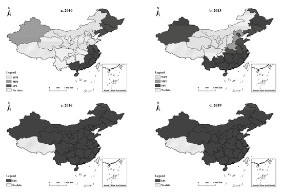
Figure 3.
Spatial distribution of the regression coefficients of population: (a) Spatial distribution of the regression coefficients of the population in 2010; (b) Spatial distribution of the regression coefficients of the population in 2013; (c) Spatial distribution of the regression coefficients of the population in 2016; (d) Spatial distribution of the regression coefficients of the population in 2019.
- 2.
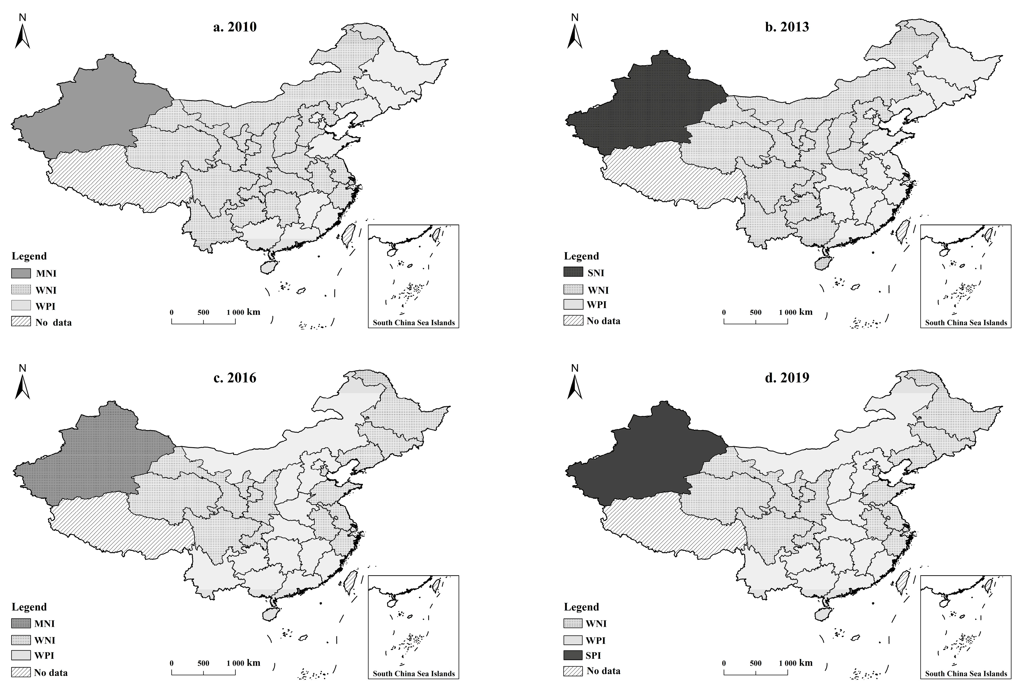
- Spatial and temporal variation in the effect of urbanization on carbon emissions
During the study period, the maximum value is 30.386 and the minimum value is −8.649. According to the influence level, it can be divided into SNI, MNI, WNI, WPI, and SPI. Overall, the urbanization rate has a predominantly negative impact on carbon emissions from public buildings. In 2010, WNI dominates, occupying 18 provinces, followed by WPI, occupying 11 provinces. In 2013, 2016, and 2019, WNI dominates, occupying 15 provinces, followed by WPI, occupying 14 provinces. It indicates that the urbanization rate has a small impact on the carbon emissions of public buildings. The scale of carbon emissions from public buildings does not increase with the increase in urbanization level; instead, it decreases with the optimization of energy consumption structure and the improvement of energy utilization efficiency. During the study period, the number of provinces with negative impact levels shows a decreasing trend, and spatially, the area of positive effect gradually expands from the northeast and some southeastern provinces to the whole eastern region, and then gradually shifts to the central region and Xinjiang province (Figure 4). Public buildings are mostly located in urban areas and less in rural areas. The increase in urbanization rate will promote the development of tertiary industry, which will further promote the generation and operation of public buildings. When the urbanization rate reaches a certain level, it will curb the carbon emissions of running public buildings because the stability of urbanization will make people start to raise the awareness of energy saving, not only limited to the use of more focus on energy efficiency.

Figure 4.
Spatial distribution of the regression coefficients of urbanization: (a) Spatial distribution of the regression coefficients of urbanization in 2010; (b) Spatial distribution of the regression coefficients of urbanization in 2013; (c) Spatial distribution of the regression coefficients of urbanization in 2016; (d) Spatial distribution of the regression coefficients of urbanization in 2019.
- 3.
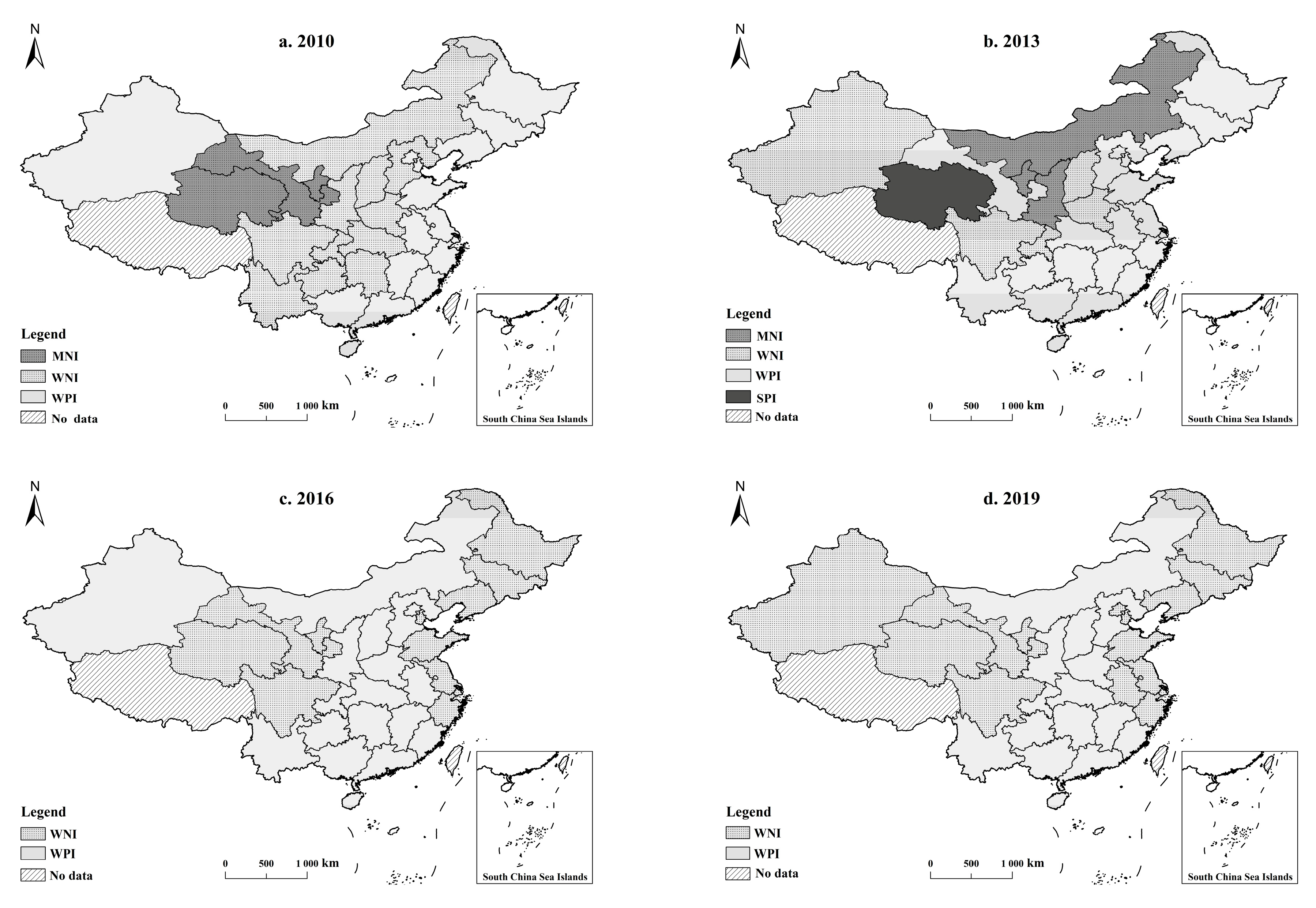
- Spatial and temporal variation in the effect of industrial structure on carbon emissions
The regression coefficient of the industrial structure has a maximum value of 0.315 and a minimum value of −0.426 in the study period. Industrial structure refers to the ratio of the value added of the tertiary sector to the total value added of production. It is classified as SPI, WPI, WNI, and MNI according to the influence level. As shown in Figure 5, it is generally a positive impact. 2010, 2013, 2016, and 2019 are dominated by weak positive impact, occupying 16, 21, 18, and 15 provinces, respectively. The positive effect of industrial structure is shifted from the east to the center. In 2010, the positive effect of industrial structure is in the eastern coastal region, northeastern region, and Xinjiang province, and that positive effect is partially shifted to the central region in 2019.
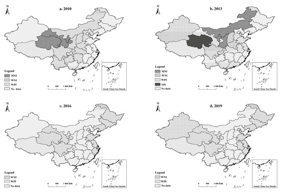
Figure 5.
Spatial distribution of the regression coefficients of industrial structure: (a) Spatial distribution of the regression coefficients of industrial structure in 2010; (b) Spatial distribution of the regression coefficients of industrial structure in 2013; (c) Spatial distribution of the regression coefficients of industrial structure in 2016; (d) Spatial distribution of the regression coefficients of industrial structure in 2019.
- 4.
- Spatial and temporal variation in the effect of GDP per capita on carbon emissions
The maximum value of the regression coefficient for GDP per capita is 1.177 and the minimum value is −1.184. In 2010, the positive effect is dominant, with a total of 16 provinces in WPI and MPI. In 2013, the negative effect is dominant, with a total of 22 provinces in SNI, MNI, and WNI. In 2016, the positive effect is more pronounced, with 24 provinces in WPI. In 2019, the positive effect is pronounced, with a total of 22 provinces in WPI and MPI. As shown in Figure 6, the influence of GDP per capita shows a trend from positive to negative and then positive again. By 2019, the only regions with a negative effect are Shanghai, Jiangsu, Zhejiang, Anhui, Fujian, Jiangxi, Hubei, and Hunan. It indicates that population affluence is promoting the increase in carbon emissions from public buildings.
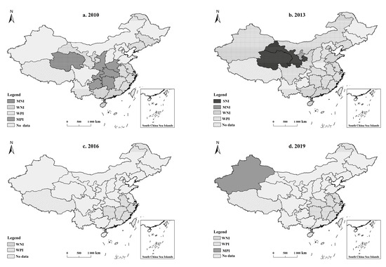
Figure 6.
Spatial distribution of the regression coefficients of GDP per capita: (a) Spatial distribution of the regression coefficients of GDP per capita in 2010; (b) Spatial distribution of the regression coefficients of GDP per capita in 2013; (c) Spatial distribution of the regression coefficients of GDP per capita in 2016; (d) Spatial distribution of the regression coefficients of GDP per capita in 2019.
- 5.
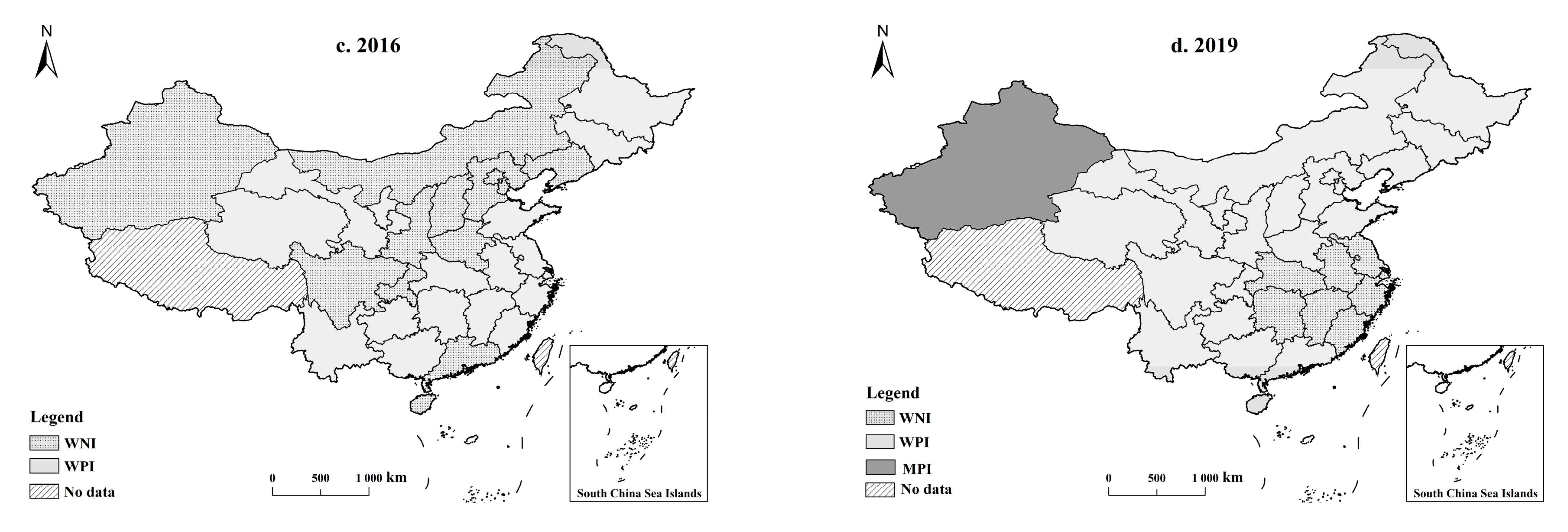
- Spatial and temporal variation in the effect of the green building index on carbon emissions
The maximum value of the regression coefficient of the green building index is 0.832 and the minimum value is −0.098. As shown in Figure 7, in 2010, all 30 provinces have a positive effect. In 2013, the WNI dominated, occupying 16 provinces. In 2016, WPI occupied 17 provinces. In 2019, WPI occupies 21 provinces. In 2010, the green building index has a positive effect on carbon emissions from public buildings in all regions. However, by 2019, the inhibitory effect has 9 provinces. According to previous studies, green buildings contribute to carbon emission reduction than non-green buildings, but this study finds that the large-scale effect of carbon emission reduction from green buildings has not yet been developed.
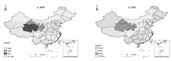

Figure 7.
Spatial distribution of the regression coefficients of the green building index: (a) Spatial distribution of the regression coefficients of the green building index in 2010; (b) Spatial distribution of the regression coefficients of the green building index in 2013; (c) Spatial distribution of the regression coefficients of the green building index in 2016; (d) Spatial distribution of the regression coefficients of the green building index in 2019.
5. Conclusions and Policy Suggestions
5.1. Conclusions
Using the carbon emission of public buildings in operation in China from 2008 to 2019, the GTWR model was used to detect the spatial distribution of the influence coefficients of population, urbanization, industrial structure, GDP per capita, and index of green buildings. We found significant spatial heterogeneity changes between the five factors. Most importantly, the factor of the index of green buildings.
The empirical results of the green building index and carbon emissions of public building operation help to determine the direction and intensity of green building development, and help to enrich the study of the impact of green buildings on the carbon emissions of public buildings from a regional perspective.
In terms of carbon emissions from public building operations, the top three public building carbon emissions from 2008–2018 were Guangdong, Jiangsu, and Beijing, and in 2019, Shandong surpassed Beijing among the top three. Overall, the total carbon emissions from public buildings in the eastern region, except Hainan, Fujian, and Tianjin, are greater than those in the central, western, and northeastern regions, and the growth rate is obvious.
The results of the hotspot analysis show that there are east-west differences in the operational carbon emissions of public buildings in Chinese provinces. The evolution of clustering shows a spatially increasing trend from west to east.
The STIRPAT model shows that population has a positive influence on public building carbon emissions in each province, and the positive influence of population gradually spreads from the northeast and the eastern coastal regions to the central and western regions; urbanization rate has a predominantly negative influence on public building carbon emissions; industrial structure has a positive influence; the influence of GDP per capita and green building index shows a trend of positive to negative and then positive; the large-scale effect of green building carbon emission reduction has not yet been formed.
5.2. Suggestions
According to the above conclusions, we can make the following recommendations.
First, total carbon emission control should be carried out at the regional level under the constraints of other indicators such as socio-economic development rate and industry economic growth. Focus on controlling carbon emission hotspot areas and emission reduction measures should be formulated for cold spot areas, according to development needs to avoid generating large amounts of carbon emissions due to rapid economic development. Cooperation between provinces can be strengthened to develop inter-provincial carbon emission trading policies to balance provincial carbon emissions.
Second, for provinces with large populations, public buildings should be retrofitted with energy efficiency. It would be advisable while developing the economy to adjust the energy consumption structure, change the economic development mode, adhere to the path of low carbon development, and slow down the rapid growth of carbon emissions caused by the rapid growth of the regional economic development level.
Third, the development of green buildings still needs to continue to improve, and the current growth of green buildings has not yet formed a scale effect on the carbon emission aspect of public buildings. Because of the high cost of green building construction, there is a need to support the construction and development of green buildings in economically disadvantaged areas.
However, this study is subject to several limitations. Firstly, this paper uses China as an example, and the analysis for green buildings can be extended to other emerging economies and developing countries. Secondly, temperature has a different impact on the heating and cooling of public buildings under different climate backgrounds. Further study can take a closer look at the micro-level of the impact of temperature on the energy consumption of public buildings. Finally, the empirical results of this paper are helpful for policy makers to develop differentiated emission reduction strategies for high and low carbon emission provincial administrative regions.
Author Contributions
Conceptualization, Z.D. and Y.L.; methodology, Z.D. and Y.L.; validation, Z.D.; formal analysis, Z.D.; data curation, Z.D. and Z.Z.; writing—original draft preparation, Z.D.; writing—review and editing, Z.D.; visualization, Z.D. and Y.L.; project administration, Z.D. and Z.Z.; funding acquisition, Y.L. All authors have read and agreed to the published version of the manuscript.
Funding
This research was funded by National Natural Science Foundation of China, grant number 71871014.
Data Availability Statement
The data used to support the results in this article are included within the paper. In addition, some of the data in this paper are supported by the references mentioned in the manuscript. If you have any queries regarding the data, the data of this study would be available from the correspondence upon request.
Conflicts of Interest
All the authors declare no conflict of interest.
References
- Nässén, J.; Holmberg, J.; Wadeskog, A.; Nyman, M. Direct and indirect energy use and carbon emissions in the production phase of buildings: An input–output analysis. Energy 2007, 32, 1593–1602. [Google Scholar] [CrossRef]
- Zhu, W.; Feng, W.; Li, X.; Zhang, Z. Analysis of the embodied carbon dioxide in the building sector: A case of China. J. Clean. Prod. 2020, 269, 122438. [Google Scholar] [CrossRef]
- China Building Energy Consumption Annual Report 2020; China Association of Building Energy Efficiency: Beijing, China, 2020.
- Zhang, Y.; Yan, D.; Hu, S.; Guo, S. Modelling of energy consumption and carbon emission from the building construction sector in China, a process-based LCA approach. Energy Policy 2019, 134, 110949. [Google Scholar] [CrossRef]
- Xiao, H.; Wei, Q.; Wang, H. Marginal abatement cost and carbon reduction potential outlook of key energy efficiency technologies in China׳s building sector to 2030. Energy Policy 2014, 69, 92–105. [Google Scholar] [CrossRef]
- Wu, X.; Peng, B.; Lin, B. A dynamic life cycle carbon emission assessment on green and non-green buildings in China. Energy Build. 2017, 149, 272–281. [Google Scholar] [CrossRef]
- Chen, L.; Xu, L.; Cai, Y.; Yang, Z. Spatiotemporal patterns of industrial carbon emissions at the city level. Resour. Conserv. Recycl. 2021, 169, 105499. [Google Scholar] [CrossRef]
- Huang, J.; Chen, X.; Yu, K.; Cai, X. Effect of technological progress on carbon emissions: New evidence from a decomposition and spatiotemporal perspective in China. J. Environ. Manag. 2020, 274, 110953. [Google Scholar] [CrossRef]
- Cui, Y.; Khan, S.U.; Deng, Y.; Zhao, M. Regional difference decomposition and its spatiotemporal dynamic evolution of Chinese agricultural carbon emission: Considering carbon sink effect. Environ. Sci. Pollut. Res. 2021, 28, 38909–38928. [Google Scholar] [CrossRef]
- Wang, L.; Fan, J.; Wang, J.; Zhao, Y.; Li, Z.; Guo, R. Spatio-temporal characteristics of the relationship between carbon emissions and economic growth in China’s transportation industry. Environ. Sci. Pollut. Res. 2020, 27, 32962–32979. [Google Scholar] [CrossRef]
- Hu, M.; Li, R.; You, W.; Liu, Y.; Lee, C.-C. Spatiotemporal evolution of decoupling and driving forces of CO2 emissions on economic growth along the Belt and Road. J. Clean. Prod. 2020, 277, 123272. [Google Scholar] [CrossRef]
- Han, Y.; Jin, B.; Qi, X.; Zhou, H. Influential Factors and Spatiotemporal Characteristics of Carbon Intensity on Industrial Sectors in China. Int. J. Environ. Res. Public Health 2021, 18, 2914. [Google Scholar] [CrossRef] [PubMed]
- Falahatkar, S.; Rezaei, F. Towards low carbon cities: Spatio-temporal dynamics of urban form and carbon dioxide emissions. Remote Sens. Appl. Soc. Environ. 2020, 18, 100317. [Google Scholar] [CrossRef]
- Bai, J.; Qu, J. Investigating the spatiotemporal variability and driving factors of China’s building embodied carbon emissions. Environ. Sci. Pollut. Res. 2021, 18, 19186–19201. [Google Scholar] [CrossRef]
- Huang, L.; Krigsvoll, G.; Johansen, F.; Liu, Y.; Zhang, X. Carbon emission of global construction sector. Renew. Sustain. Energy Rev. 2018, 81, 1906–1916. [Google Scholar] [CrossRef] [Green Version]
- Lu, Y.; Cui, P.; Li, D. Carbon emissions and policies in China’s building and construction industry: Evidence from 1994 to 2012. Build. Environ. 2016, 95, 94–103. [Google Scholar] [CrossRef]
- Wu, Y.; Shen, L.; Zhang, Y.; Shuai, C.; Yan, H.; Lou, Y.; Ye, G. A new panel for analyzing the impact factors on carbon emission: A regional perspective in China. Ecol. Indic. 2019, 97, 260–268. [Google Scholar] [CrossRef]
- Mostafavi, F.; Tahsildoost, M.; Zomorodian, Z. Energy efficiency and carbon emission in high-rise buildings: A review (2005–2020). Build. Environ. 2021, 206, 108329. [Google Scholar] [CrossRef]
- Tan, X.; Lai, H.; Gu, B.; Zeng, Y. Carbon emission and abatement potential outlook in China’s building sector through 2050. Energy Policy 2018, 118, 429–439. [Google Scholar] [CrossRef]
- Wang, M.; Feng, C. Exploring the driving forces of energy-related CO2 emissions in China’s construction industry by utilizing production-theoretical decomposition analysis. J. Clean. Prod. 2018, 202, 710–719. [Google Scholar] [CrossRef]
- Huang, W.; Li, F.; Cui, S.-H.; Huang, L.; Lin, J.-Y. Carbon Footprint and Carbon Emission Reduction of Urban Buildings: A Case in Xiamen City, China. Procedia Eng. 2017, 198, 1007–1017. [Google Scholar] [CrossRef]
- Rose, T.D.E.A. Effects of population and affluence on CO2 emissions. Ecology 1997, 94, 175–179. [Google Scholar]
- Ma, M.; Shen, L.; Ren, H.; Cai, W.; Ma, Z. How to Measure Carbon Emission Reduction in China’s Public Building Sector: Retrospective Decomposition Analysis Based on STIRPAT Model in 2000–2015. Sustainability 2017, 9, 1744. [Google Scholar] [CrossRef] [Green Version]
- Ma, M.; Yan, R.; Cai, W. An extended STIRPAT model-based methodology for evaluating the driving forces affecting carbon emissions in existing public building sector: Evidence from China in 2000–2015. Nat. Hazards 2017, 89, 741–756. [Google Scholar] [CrossRef]
- Yang, X.; Jia, Z.; Yang, Z.; Yuan, X. The effects of technological factors on carbon emissions from various sectors in China—A spatial perspective. J. Clean. Prod. 2021, 301, 126949. [Google Scholar] [CrossRef]
- Dietz, T.; Rosa, E.A. Rethinking the Environmental Impacts of Population, Affluence and Technology. Hum. Ecol. Rev. 1994, 1, 277–300. [Google Scholar]
- York, R.; Rosa, E.A.; Dietz, T. STIRPAT, IPAT and ImPACT: Analytic tools for unpacking the driving forces of environmental impacts. Ecol. Econ. 2003, 46, 351–365. [Google Scholar] [CrossRef]
- Yan, H.; Liu, H.; Qiu, R.; Zhang, Y. Influencing Factors Analysis of Construction Industry Carbon Emissions Based on Stepwise Regression. J. Eng. Manag. 2021, 35, 16–21. [Google Scholar]
- Zhang, S.; Wang, K.; Yang, X.; Xu, W. Research on Emission Goal of Carbon Peak and Carbon Neutral in Building Sector. Build. Sci. 2021, 37, 189–198. [Google Scholar]
- Xie, J. Discussion on Peak Carbon Emissions and Energy Saving-Emission Reduction of Public Buildings in Chongqing Based on LEAP Model; Chongqing University: Chongqing, China, 2019; p. 103. [Google Scholar]
- Jiang, X. Study on Forecast and Factor Decomposition of Carbon Emissions about Chinese Large-Scale Public Buildings; Ocean University of China: Chongqing, China, 2012; p. 74. [Google Scholar]
- Xiao, H.; Yi, D. Empirical Study of Carbon Emissions Drivers Based on Geographically Time Weighted Regression. Model. Stat. Inf. Forum. 2014, 29, 83–89. [Google Scholar]
- Yang, D.; Liu, B.; Ma, W.; Guo, Q.; Li, F.; Yang, D. Sectoral energy-carbon nexus and low-carbon policy alternatives: A case study of Ningbo, China. J. Clean. Prod. 2017, 156, 480–490. [Google Scholar] [CrossRef]
- Lin, F.J.Z. Spatiotemporal distribution and provincial contribution decomposition of carbon emissions for the construction industry in China. Resour. Sci. 2019, 41, 897–907. [Google Scholar]
- Cheng, Z.; Li, L.; Liu, J. Industrial Structure, Technical Progress and Carbon Intensity in China’s Provinces. Renew. Sustain. Energy Rev. 2018, 81, 2935–2946. [Google Scholar] [CrossRef]
- Wang, H.; Zhang, B.; Liu, Y.; Liu, Y.; Xu, S.; Deng, Y.; Zhao, Y.; Chen, Y.; Hong, S. Muti-dimensional analysis of urban expansion patterns and their driving forces based on the center of gravity-GTWR model: A case study of the Beijing-Tianjin-Hebei urban agglomeration. Acta Geogr. Sin. 2018, 73, 1076–1092. [Google Scholar]


Publisher’s Note: MDPI stays neutral with regard to jurisdictional claims in published maps and institutional affiliations. |
© 2022 by the authors. Licensee MDPI, Basel, Switzerland. This article is an open access article distributed under the terms and conditions of the Creative Commons Attribution (CC BY) license (https://creativecommons.org/licenses/by/4.0/).