Benchmark of Electricity Consumption Forecasting Methodologies Applied to Industrial Kitchens

Abstract

Even though Industrial Kitchens (IKs) are among the highest energy intensity spaces, very little work has been done to forecast their consumption. This work explores the possibility of increasing the accuracy of the consumption forecast in an IK by forecasting disaggregated appliance consumption and comparing these results with the forecast of the total consumption of these appliances (Virtual Aggregate—VA). To do so, three different methods are used: the statistical method (Prophet), classic Machine Learning (ML) method such as random forest (RF), and deep learning (DL) method, namely long short-term memory (LSTM). This work uses individual appliance electricity consumption data collected from a Portuguese restaurant over a period of four consecutive weeks. The obtained results suggest that Prophet and RF are the more viable options. The former achieved the best performance in aggregated data, whereas the latter showed better forecasting results for most of the individual loads. Regarding the performance of the VA against the sum of individual appliance forecasts, all models perform better in the former. However, the very small difference across the results shows that this is a viable alternative to forecast aggregated consumption when only individual appliance consumption data are available.

1. Introduction

The global demand for electricity continues to increase, and strong economic growth, combined with more extreme weather conditions than in 2020, increased the demand by 6% in 2021 [1]. Despite efforts made in recent years regarding the development and implementation of RES, electricity generation from coal- and gas- based electricity generation reached record levels [1]. As a result, the annual greenhouse gas emissions of the global electricity sector reached the highest ever recorded value [1]. Contributing to this phenomenon are energy-intensive businesses with an underestimated consumption [2], such as IKs. Despite the high energy usage of IKs [2,3], very little research exists related to their consumption and energy reduction strategies [4].

To mitigate the contribution of IKs to greenhouse gas emissions, and given that forecasting energy consumption helps to increase the penetration of RES thanks to better coordination of generation and electricity consumption, this work explores new methodologies of forecasting power consumption in IKs to study if there is room to improve the performance of said forecast.

In the present work, real-world data are obtained through a monitoring system. However, some small loads are not equipped with sensors. Because of that, the total consumption is slightly different from the consumption of the monitored appliances. Hence, the concept of VA is proposed. VA refers to the power demand of the restaurant, defined as the sum of loads of each individual appliance monitored in the restaurant. It is different from the real aggregate (the measured value for the total load) because it does not include certain elements that are not directly associated with the IKs, e.g., the lighting of the dining room.

The main goal of this work is to explore the possibility to improve the electricity consumption forecast in an unexplored and energy-intensive area. Finding suitable forecasting methods for the effective management of energy resources improves the efficiency of energy consumption and decreases its impact on the environment [5]. To this end, the proposed forecasting methodology aims to assess whether there is an improvement in the forecast results using three different methods to forecast both the virtual aggregate and the individual appliances. The forecasts of the individual appliances are then summed and compared with the forecast of the virtual aggregate. Finally, the three different algorithms are compared to see which performed better. All forecasts are made for a one-hour horizon.

The remainder of this paper is organized as follows: The state of the art concerning energy consumption in IKs and forecasting of electricity demand is presented in Section 2. Section 3 presents the dataset used and the research methods used. The results obtained are presented and discussed in Section 4. The paper concludes in Section 5 with a discussion of the main limitation of the presented methodology and and outline of future work possibilities.

2. State of the Art

2.1. Electricity Management in Industrial Kitchens

According to Mudie et al. [2], electricity consumption in IKs is much greater than the literature suggests. Kitchen- and food-related activities outweigh other energy-consuming activities [3]; furthermore, the carbon footprint of the contract catering sector is 80% higher than initial estimates [4].

A study developed by Higgins et al. showed that most of the literature on sustainability in restaurants is limited to ecological aspects, rather than a holistic approach [6]. This limits the possibility of achieving more sustainable restaurant options. There are, however, some exceptions to this; in 2017, a holistic evaluation of the carbon and energy impact of different food preparation options in delivering a restaurant’s menu was carried out [7]. After considering seven energy reduction scenarios, the study estimated that up to 58% of energy could potentially be saved.

Regarding the introduction of RES in the operation of IKs, research is very scarce. Most of the work is related to the use of biomass fuel from industrial kitchen waste or the implementation of heat recovery systems. Similarly, by searching for the exact desired result: “implementation of renewable energy in industrial kitchens”, there is no related work in the first four pages of the search engine. When changing the keyword “industrial” to “commercial”, a few results are found. On contrary, several works can be found concerning the integration of RES in houses [8] and buildings [9].

Among the works that were found, one of them considered two buildings composed of a mix of apartments and one commercial kitchen [10]. These buildings are connected to a small-scale microgrid that includes renewable energy generation and electric storage. The microgrids are composed of photovoltaic arrays and wind turbines, as well as an additional backup, by being connected either to the grid or to a backup diesel generator. Microgrid sizing and costs are generally sensitive to load shape [10]. The research showed that by implementing thermal storage there was the potential to increase renewable penetration by 7% and decrease renewable curtailment (renewable energy resources that cannot be utilized and are therefore wasted) by 11% [11], indicating that multiple types of storage can benefit the penetration of renewable energy. Although the goal is to have a building with 100% penetration of renewable energy sources, sometimes this is not the most economically viable option. The work conducted by Aldaoubab et al., after performing an economic analysis, demonstrates that lowering the desired penetration from 100% to 80% cuts the energy cost significantly [10] due to the required sizing of the microgrid. The economic aspect is a crucial concept in moving towards 100% penetration of renewable energy.

2.2. Electricity Consumption Forecasting

Electricity consumption forecasting is a crucial aspect of energy planning, management, and optimization, with the goal of increasing efficiency and decreasing consumption. As mentioned above, the amount of work carried out regarding energy consumption in IKs is not abundant. Still, power demand forecasting is a very explored topic (especially for household power demand), and many different approaches have been taken to predict a load demand curve. The three main approaches to building energy consumption and modeling forecasting can be classified as physics-based, data-driven, and hybrid models [12]. The work presented in this paper focuses on data-driven models.

Data-driven models can be divided into statistical or conventional models and ML models. The latter can be separated into shallow ML and the most recent DL techniques. Next, a survey of some of the existing literature on this topic is presented.

Two popular methods of building energy consumption model forecasting are autoregressive models and statistical regression. They provide a good balance between simplicity of implementation and precision of forecasting. They have limitations with respect to the forecasting horizon and modeling nonlinear data patterns [12]. ARIMA and many of its modifications can be seen being used to forecast energy consumption in buildings. Some examples of these are from Newsham and Birt [13], Yun et al. [14].

A more recently developed regression model is Prophet [15]. Prophet is a modular regression model with interpretable parameters. This algorithm has been used to predict power demand in various works and in different ways. In [16,17], a hybrid prophet–LSTM model is presented to forecast electric demand. In [18], Prophet has been used for real-time day-ahead consumption forecasts, while [19] implemented a long-term forecast (one year or beyond) that performed outstandingly in metrics such as accuracy, generalization, and robustness.

Several ML techniques have been used to forecast energy consumption in buildings. A popular technique is SVM. They are efficient for nonlinear problem solving and offer accurate results even with smaller datasets [12]. In [20], the authors forecast the demand for cooling and heating energy with exogenous input variables using an SVM. The research showed that appropriate input data selection could improve forecast accuracy. Similar conclusions were drawn from the research carried out in [21]. Here, a short-term forecast was carried out for a university building in Spain, comparing the results of three different methods: SVM, MLP, and multilinear regression. The SVM model showed higher accuracy and, again, the accuracy of the model increased with an appropriate selection of variables.

Moreover, DTs is used to forecast energy consumption in buildings. DTs follow the idea of a tree, from the roots to the leaves. There is an initial root node, where depending on the conditions established it diverges into other nodes, which can again diverge into more nodes until it reaches a leaf (a valid classification or forecast value). Many different types of DT have been developed, each with its own virtues and utility. In [22], a comparison of stepwise regression models, MLP and DT, is carried out to forecast the electrical load of residential households. Here, the DTs proved to be the most accurate during the summer period, although it was outperformed in the winter.

Another technique used to forecast energy consumption in buildings is ensemble models. Ensemble models can be either homogeneous or heterogeneous. Homogeneous modeling creates subsamples of the original dataset, which are then processed by one single data-driven technique [12]. Heterogeneous modeling on the other hand uses a number of different forecasting algorithms trained on the same dataset, the forecasting results from each model are then weighted to give the final output.

Similarly to a DTs, but with its own characteristics, is RF. An RF is considered an ensemble homogeneous model. An advantage over a conventional DT is that it corrects the tendency to overfit the training set. It does so by generating a group of several DTs whose results are aggregated into one [23]. They usually implement randomization on two different levels by having each DT trained with a random subset of observations and then having each tree node divided by considering a random subset of variables [12]. RF is used to forecast energy consumption in buildings in several papers, such as [24] or [25].

DL techniques have seen their popularity increase in recent years, mainly due to their ability to handle large amounts of data, their improved feature extraction abilities and, consequently, improved model performances [26]. Runge and Zmeureanu [26] conducted a review of deep learning techniques used in forecasting energy use in buildings. This review showed that the most popular techniques used are AEs and RNNs.

LSTM neural networks, a special type of RNN, are among the most popular DL architectures and have been used before to forecast energy consumption in buildings, or even whole districts. For example, in [27], LSTM models were compared with other prominent data-driven models for short-term residential load forecasting, and their experiment showed the LSTM model obtained the lowest forecasting error. In [28], twelve different shallow algorithms and DL were used to predict the cooling load of the building. The study showed that LSTM and extreme gradient boosting were among the most accurate models. More research using the LSTM forecast is conducted in [29], where a forecast energy consumption for an educational building is presented, showing different LSTM-based models outperformed SVM, deep belief networks, and ARIMA models.

Concerning the characterization and monitoring of building energy demand, several methods can be adopted. In [30], the use of a statistical process with the aim of signaling alarms and detecting faults of unexpected energy demand was proposed. More recently, in [31], Bayesian linear regression methodology has been proposed for modeling and characterization in tertiary buildings. The main conclusion achieved by the authors in [31] is that the methodology is intuitive and explainable and provided accurate baseline predictions. Requirements of forecasting models for smart grids and buildings are reviewed in [32].

2.3. Summary

To summarize, it is clear from the state of the art that there is an important research gap to address when it comes to assessing the forecasting of electricity demand in IKs. Furthermore, it is also possible to conclude that there is not a clear winner when it comes to selecting the most adequate forecasting algorithms for demand forecasting on domains other than IKs. The work in this paper is to the best of the authors’ knowledge one of the first works that benchmark forecasting algorithms using data from an IK being operated in real-world conditions.

3. Materials and Methods

3.1. Forecasting Algorithms

Considering the results presented in the literature review, it was decided to evaluate the performance of an algorithm in each of the three categories. More precisely, we used some of the most common benchmarks in each category: Prophet for statistical models, RF in shallow ML models, and LSTM in DL models.

3.1.1. Prophet

Prophet is a modular regression model which is designed to have intuitive parameters that can be adjusted without knowing the details of the underlying model [15]. It uses a decomposable time series model with three main components: trend, seasonality, and holidays. Equation (1) shows how these elements are combined. Where $g\left(t\right)$ is the trend function, it models nonperiodic changes in the value of the time series. Here $s\left(t\right)$ represents periodic changes (such as weekly or yearly seasonality), and $h\left(t\right)$ represents the effect of holidays that occur irregularly on the schedule. The error is represented by $ϵ\left(t\right)$.

$$y\left(t\right)=g\left(t\right)+s\left(t\right)+h\left(t\right)+ϵ\left(t\right)$$

(1)

This forecasting methodology offers various advantages. Most notably, the fact that seasonality is accommodated by default for multiple periods and the fact that the fitting is very fast. Hence, allowing near-real-time training and inference.

In this work, the Prophet algorithm was implemented in two different forms. iN One way, the model is trained with the entire training set in one go and makes a three-day forecast horizon (the whole test set). This method uses the same amount of training data as the LSTM and RF methods (all of the data available for February) but has a larger forecasting horizon. The other way this was implemented was by training with the training set and by taking advantage of how quickly it can be trained. In this case, the model is retrained in each window with newly available data and forecasts for the next 12 data points (one hour). This algorithm was implemented in Python using the Prophet library. Prophet is available on https://facebook.github.io/prophet/docs/quick_start.html#python-api (accessed on 5 September 2022).

3.1.2. Random Forest

RFs are usually implemented through randomization on two different levels by having each DT trained with a random subset of observations and then having each tree node divided by considering a random subset of variables [12]. For a random vector X representing the input of real data and a variable Y representing the response of the real value, the goal is to find a prediction function $f\left(X\right)$ to predict Y. The ensembles construct f in terms of a collection of so-called “base learners”. These base learners are combined to give the ensemble predictor $f\left(x\right)$. For regression, the final output $f\left(x\right)$ comes from the average of all the base learners.

RFs offers various computational and statistical advantages, such as relatively fast (e.g., when compared with Neural Networks) training procedures. RFs also have built-in generalization error estimates and are able to impute missing values by default [33]. Another very relevant advantage is that it depends only on a few hyper-parameters, since according to [33], only three parameters need to be tuned to improve the accuracy of the model; m, the number of randomly selected predictor variables; J, the number of trees; and tree size, as measured by the smallest node size for splitting or the maximum number of terminal nodes.

In this work, this method was implemented following the windowing method described in Section 3.3.1, using Python as a programming language and the Scikit-learn RandomForestRegressor Random Forest Regression, https://scikit-learn.org/stable/modules/generated/sklearn.ensemble.RandomForestRegressor.html (accessed on 12 September 2022).

3.1.3. Long Short-Term Memory Deep Neural Network

The LSTM model is an RNN specially designed to overcome the problems of the exploding/disappearing gradient that typically arise when learning long-term dependencies [34]. A basic LSTM unit is composed of a cell, an input gate, an output gate, and a forget gate. The latter allows the network to reset its state; this gate was not initially part of the LSTM but was later introduced [34]. The cell remembers values over arbitrary time intervals, and the three gates regulate the flow of information associated with the cell.

The main idea behind the memory block is to maintain its state over time and regulate the information flow through nonlinear gating units. The output of the block is recurrently connected to the input block and all gates [34], which means that the input to the LSTM block will be a combination of the current input $x_t$ and the previous output of the LSTM $y\left(t-1\right)$.

The same windowing methodology applied to the RF algorithm is used here. This technique was implemented in Python using the LSTM library from “keras” LSTM, https://keras.io/api/layers/recurrent_layers/lstm/ (accessed on 19 September 2022).

3.2. Dataset

This paper uses electricity consumption data taken from one restaurant in a region of southern Europe [35]. The electrical demand for the individual appliances was collected using the smart meter at the circuit level of the E-Gauge eGauge, https://www.egauge.net/ (accessed on 27 June 2022). A total of 18 appliances were individually monitored for nearly one month. For each appliance, active power and reactive power (in each line if it is a three-phase appliance) are measured.

The available data range from the sixth of February of 2019 at 00:00 (6 February 2019 00:00:00) to the fourth of March at 08:47 (4 March 2019 08:47:17). The data were originally collected at the rate of one sample every five seconds. A summary of the available data can be seen in

Table 1. Summary of the appliance-level data that constitute the dataset.

	Max Power (W)	Avg. Power (W)	Null Samples
Blast Chiller	5331	215	8056 (1.88%)
Infrared Lights	1133	211	147 (0.03%)
Dish Washer	4456	480	1949 (0.45%)
Glass Washer	1885	43	4 (0.001%)
Convection Oven 1	8797	386	7044 (1.64%)
Convection Oven 2	8337	382	7344 (1.71%)
Salamander 1	3148	944	5995 (1.4%)
Salamander 2	3182	526	6819 (1.59%)
Dual Fryer	5222	219	2619 (0.61%)
Freezer	1319	577	7936 (1.85%)
Ice Machine	421	143	7433 (1.73%)
Mise en Place	854	219	8073 (1.88%)
Garde Manger 1	1278	180	8232 (1.92%)
Garde Manger 2	418	70	8075 (1.88)
Refrigerator—Drinks	623	145	17 (0.004%)
Refrigerator—Fish	3709	96	107 (0.02%)
Refrigerator—Meat	1274	132	54 (0.01%)
Refrigerator—Vegetables	897	99	146 (0.03%)

. As can be observed, every appliance has null measurements due to issues with the data collection platform. Most of these were consecutive and were located in the first days of the dataset; therefore, every data point before to the 5th of February was eliminated. The remaining null data points were dealt with using a forward fill function as described next.

Data Preprocessing

The initial step is to perform a preprocessing of the data. This includes methods to handle null values and outliers, data resampling, creation of the virtual aggregate, and data normalization. Null values appeared in the dataset in two different forms, a large cluster of them in the first few days and some scattered throughout the data set. To deal with the first, the data from the days including the cluster of missing values and the previous days were simply removed from the dataset. To deal with the latter, a forward fill function was carried out (filling a null value with the previous valid value). The resulting data were then averaged to 5 min resolution. After this step, VA was created by adding the power consumption of each appliance at each instant of time t according to Equation (2). A median filter was also applied to reduce the inevitable noise from the measurement process.

$$V{A}_x\left(t\right)=\sum X_a\left(t\right)$$

(2)

Finally, normalization of the data was carried out for each of the individual appliances and the VA. This work took a max normalization approach in which all values are rescaled between 0 and 1 by undergoing the process in Equation (3), where x is the total dataset and $x_i$ is the value of the data point at instant i. This method allows for easy interpretability of the resulting forecast and its performance metrics. Moreover, it is easy to rescale to the original values.

$$x_{i,normalized}=\frac{x_i}{max\left(x\right)}$$

(3)

3.3. Performance Evaluation Methodology

One of the main goals of this work is to understand whether forecasting consumption of individual appliances and summing these forecasts can improve the forecast compared with forecasting VA directly. With that goal in mind, the models for each appliance are individually evaluated, and then a model for VA is created and evaluated. Finally, the outputs of the individual appliances are added and compared with the performance of the VA model. To be able to compare and draw conclusions from the forecasts, it is necessary to obtain performance metrics of these. This section describes the process of training and testing and the selection of an appropriate performance metric for the problem at hand.

3.3.1. Training and Testing Procedures

Due to the short size of the dataset, it was decided to split the data with 85% for training and 15% for testing (roughly 3 days). It was also decided that a validation set would be used in the training of the LSTM model only. This is because LSTM models have more hyper-parameters to train and can benefit more from the implementation of a validation set to avoid overfitting. This validation set consists of the last day of the training set, shortening the training set and not the already thin test set. It was also decided that only consecutive days would be considered in the training and test sets. To this end, any days that did not have 288 samples after the preprocessing set were discarded. The fact that only full days are used to train ensures that the model has had the same amount of data to learn the consumption patterns at different times of the day, and it is important that these are consecutive days, since the consumption at the end of one day is always followed by the beginning of the next day, and there still could be relationships here, even though this time of the day is of less interest than when the restaurant is operating.

This being said, the next step was to prepare the training and test set, which were different for the different algorithms. More precisely, for RF and LSTM, it was first necessary to split the training and test set into consecutive windows of forecasting inputs and outputs (i.e., the targets). In this work, the size of the input data was set to one day (i.e., 288 samples of 5 min aggregates), while the output size was set to 1 h (12 samples). This approach is not necessary for the Prophet algorithm, since it takes as input the entire training set.

3.3.2. Performance Metrics

Two popular performance metrics are RMSE and MAE, shown in Equations (4) and (5). Where n is the number of samples, y is the target value, and $\widehat{y}$ is the forecasted value. Despite both metrics being used to assess model performance for many years, there is no consensus on the most appropriate metric for forecasting problems [36]. While the MAE gives the same weight to all errors, the RMSE penalizes variance, as it gives errors with larger absolute values more weight than errors with smaller absolute values. One major concern to use the RMSE as a performance metric is its sensitivity to outliers. Some researchers affirm that by giving a higher weighting to unfavorable conditions, RMSE is usually better at revealing model performance differences, and another advantage is that RMSE avoids the use of absolute values, which are undesirable in many mathematical calculations [36]. The underlying assumption when presenting RMSE is that the errors are unbiased and follow a normal distribution [36].

$$RMSE=\sqrt{\frac{1}{n}\sum _{i=1}^n{(y_i-{\widehat{y}}_i)}^2}$$

(4)

$$MAE=\frac{1}{n}\sum _{i=1}^n\left|y_i-{\widehat{y}}_i\right|$$

(5)

Since our dataset is bound to be very diverse (individual appliances are going to have distinct consumption patterns from one another), it is hard to select a performance metric that will satisfy all needs. With all this taken into account, it was decided to measure the error in the forecast by using both RMSE and MAE to obtain more knowledge of the performance of the developed models.

4. Results and Discussion

This section presents and discusses the obtained results. First, the results for VA are presented, followed by the results of the individual appliances. Then, the performance of VA is compared with that by summing the forecasts of the individual appliances. Finally, a discussion on the overall results is also provided.

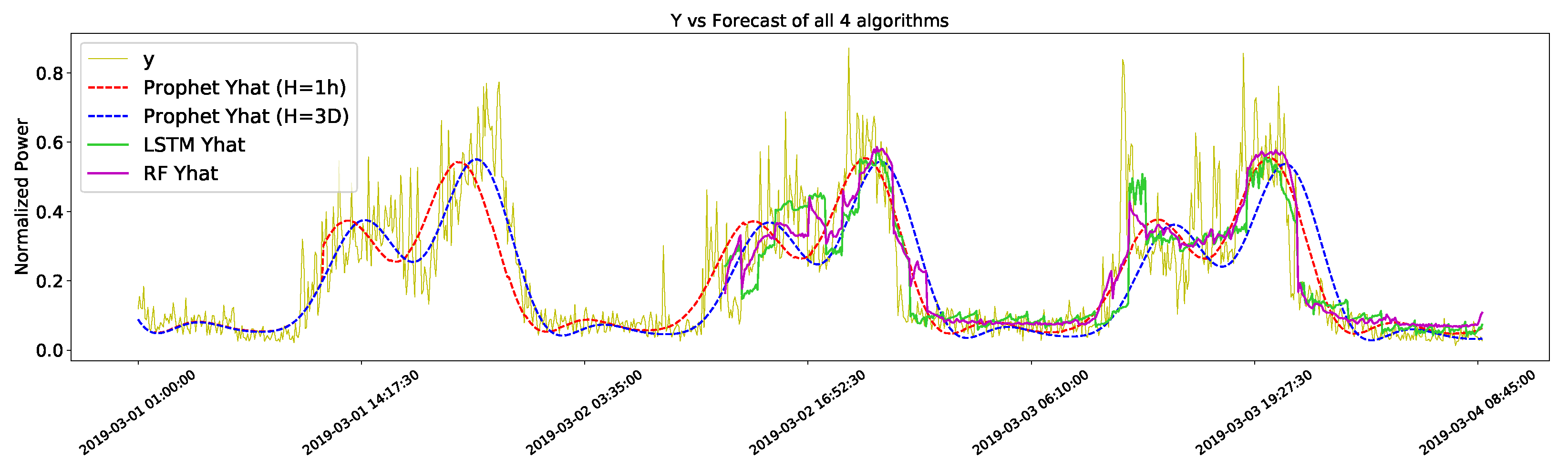
4.1. Virtual Aggregate Forecast

Figure 1 shows the forecast of all four methods against the test set. Both the Prophet forecasts for the one-hour time horizon (H = 1 h) and three-day time horizon (H = 3D) show a much smoother pattern than those of the RF and LSTM forecasts. From this figure, it is hard to tell which algorithms performed better, and for this reason,

Table 2. Performance metrics of different algorithms’ comparison for the normalized virtual aggregate.

	Prophet (H = 3D)	Prophet (H = 1 h)	RF	LSTM
RMSE	0.10	0.12	0.10	0.11
MAE	0.073	0.068	0.066	0.066

is included in the performance metrics of each method.

One can see here that the Prophet performed better with a shorter horizon and more data to train. This was somewhat expected, since short-term forecasts tend to be more accurate than long-term forecasts. Overall, the best performer was RF. However, the differences in performance are very short, hence it is not possible to say that one is better than the other.

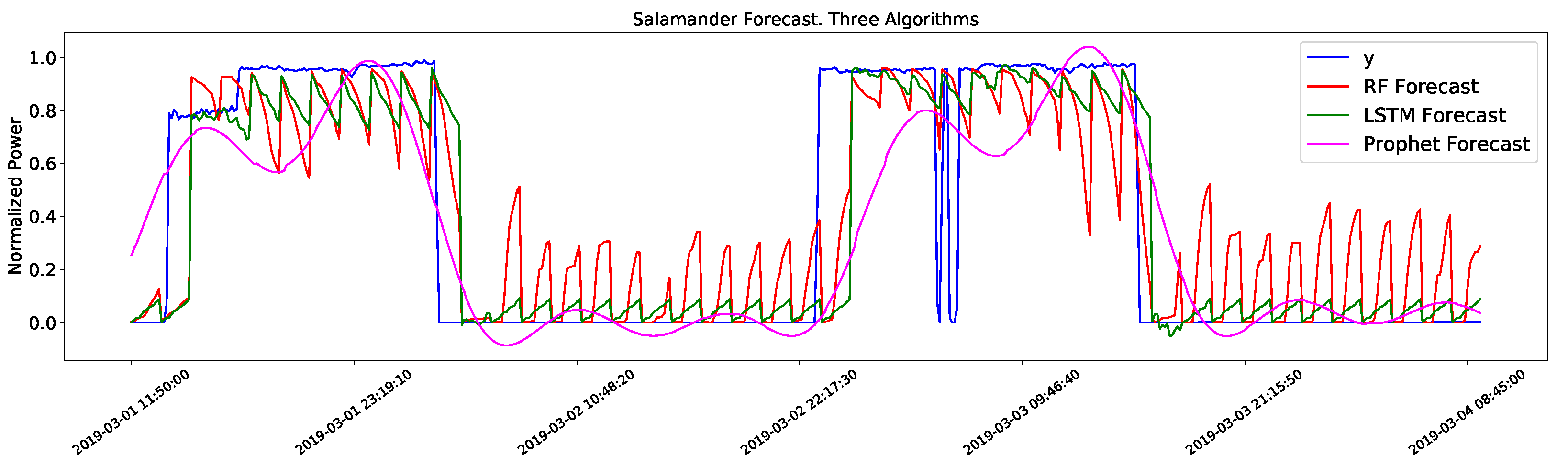
4.2. Individual Appliances Forecast

The NRMSE scores for the individual appliance forecasts are presented in

Table 3. Performance metrics of different algorithms’ comparison for individual appliances (NRMSE).

	Prophet (H = 3D)	Prophet (H = 1 h)	RF	LSTM
Blast Chiller	0.20	0.17	0.15	0.17
Infrared Lights	0.31	0.26	0.24	0.25
Dish Washer	0.20	0.19	0.20	0.21
Glass Washer	0.06	0.05	0.0002	0.005
Convection Oven 1	0.14	0.13	0.14	0.14
Convection Oven 2	0.13	0.13	0.15	0.13
Salamander 1	0.34	0.25	0.25	0.22
Salamander 2	0.24	0.21	0.15	0.17
Dual Fryer	0.08	0.08	0.08	0.08
Freezer	0.28	0.12	0.097	0.10
Ice Machine	0.31	0.31	0.29	0.31
Mise en Place	0.34	0.33	0.26	0.28
Garde Manger 1	0.18	0.18	0.16	0.17
Garde Manger 2	0.19	0.19	0.18	0.19
Refrigerator—Drinks	0.32	0.32	0.27	0.29
Refrigerator—Fish	0.21	0.21	0.23	0.22
Refrigerator—Meat	0.21	0.21	0.22	0.22
Refrigerator—Vegetables	0.18	0.18	0.17	0.17

, where the green values are the best performers for that appliance, while the red value is the worst. As it can be observed, individual appliance forecasts yield higher errors when compared with the virtual aggregate forecast. The exception is the glass washer, which due to being turned OFF during the test period has a very good performance.

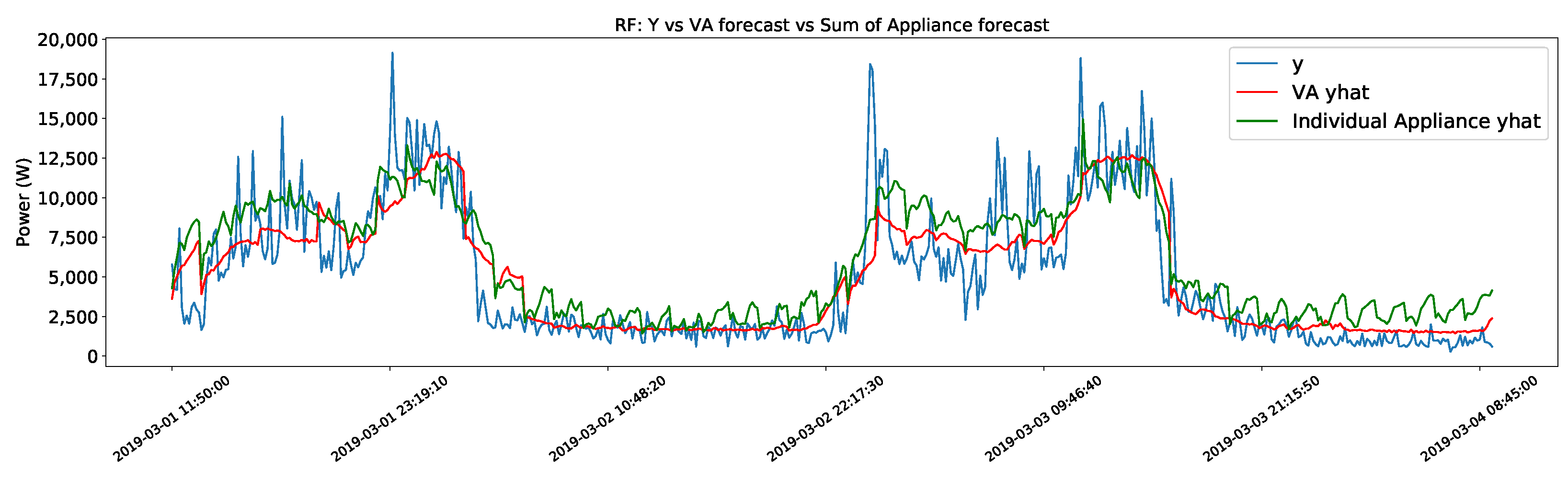
4.3. Virtual Aggregate Forecast vs. Sum of Individual Loads Forecast

Given that the Prophet algorithm for a time horizon of one hour outperformed the algorithm for a time horizon of three days in almost every case, the following analysis considers only this model for the Prophet. The results of the forecast of VA and the sum of the forecast for individual appliances are shown in

Table 4. Performance metrics of different algorithms’ comparison for the normalized virtual aggregate.

	RMSE	MAE
Prophet (H = 1 h)-Virtual Aggregate	2290	1499
Prophet (H = 1 h)-Individual Appliances	2287	1507
RF—Virtual Aggregate	2230	1507
RF—Individual Appliances	2520	1998
LSTM—Virtual Aggregate	2461	1564
LSTM—Individual Appliances	2630	1961

. Overall, the error of the forecast for all the algorithms was smaller when forecasting for the VA rather than summing the forecast of the individual appliances.

Several reasons could be attributed to why the VA forecast performed better than the sum of the individual appliances forecast. These are now be discussed. Firstly, the amount of data available for this work was not very large (roughly one month of data available). This especially affects the LSTM model, which thrives on large datasets. Although this issue affects both the forecast of the VA and the individual appliance, the load of the IK is much more stable over time than the load of most appliances. This virtually aggregated load always follows the same pattern: peak values at lunchtime and dinnertime followed by a valley until the next lunchtime. However, these patterns are not visible in most appliances, making it much harder for the forecasting algorithms to learn an accurate model for each appliance.

This leads to the second issue; the forecast of power consumption in certain appliances with a binary behavior (e.g., constant consumption when ON). The methods are incapable of following this kind of trend and forecast a saw pattern instead. This can be seen in Figure 2, where the target value changes between two values, and the algorithms fail to follow this trend (especially the RF algorithm). All three methods are able to predict when the appliance is ON but can not predict the correct value. The impact this has on the sum of the prediction of the individual appliances can be seen in Figure 3 and is one of the reasons why the prediction for VA has a smaller error.

Moreover, it is worth mentioning the comparison of the Prophet algorithm for VA with the sum of the forecasts for the individual appliances seen in Figure 4. Both forecasts follow almost identical curves. While it is not in the scope of this work to go into detail on the mathematics behind the functioning of the Prophet model, this result indicates that Prophet works in a way that the sum of the parts is equal to the whole. This could presumably change if the parameters of the model (such as seasonality) were changed for each specific appliance.

4.4. Discussion

All three algorithms benchmarked in this work have their own merits. Prophets’ performance is peculiar; it is the easiest algorithm to implement, and its performance is almost identical when forecasting the sum of individual appliances or the VA. This makes it so that when making the comparison of forecasts of the individual appliances using the three different methods, Prophet outperforms the other two, measured both in RMSE (2287 W against 2520 W in RF) and MAE (1507 W against 1998 W in RF). However, comparing the accuracy of the VA forecast is a more difficult call. It presents the smallest MAE (1499 W versus 1507 W in RF) but the second-best RMSE (2290 W versus 2230 W in RF).

RF shows an overall good performance forecast for the appliances. It has the best forecasting accuracy for 10 out of 17 of the appliances, more than the other algorithms combined (in contrast, the Prophet is the worst in 10 out of 17). This makes it the best option when the objective is to forecast a concrete set of appliances. Moreover, its performance on the VA was one of the best. In contrast, the LSTM was one of the weakest performing models. It has the largest RMSE for both the VA and the sum of the individual appliances. It does, however, score better than RF when measured with MAE for the sum of individual appliances. This is mainly because it outperforms RF when forecasting for some of the appliances with binary behavior, as can be seen in Figure 2. The low accuracy of this model can surely be associated with the low amount of available data, on which LSTM networks thrive. However, from our experiments, it is clear that LSTMs are a viable option to explore further.

Regarding the performance of the forecast of VA versus the sum of the forecast of the individual appliances, from the results obtained, it is not possible to conclude that the forecast was improved by forecasting for the individual appliances. The three algorithms performed better forecasting for VA. However, this does not mean that there are no advantages to the proposed methodology. In fact, the ability to forecast the aggregate by considering the sum of individual appliances allows the user to add or remove loads from the aggregated forecast without the need to retrain the entire model. Instead, only the new appliance needs a newly trained model, while the data of the already existing appliances remain relevant. When models are trained only for VA, the inclusion of a new appliance will potentially disrupt the new consumption pattern, hence damaging the prediction ability of the model. Considering that restaurants are changing businesses, with new appliances being added or removed with a higher frequency than that of residential kitchens, this is a very important aspect to consider. This advantage is maintained when removing an appliance from the restaurant (for maintenance reasons, for example), since in this case, one can simply remove the forecast for the said appliance from the mix.

Another advantage of this method is that it enables the creation of forecasts for different consuming sectors of the restaurant. This means that one can agglomerate the consumption of the freezers or the ovens, for example, and study consumption in this manner. Finally, this methodology allows for the forecast of each appliance to be fine-tuned. Each appliance has its own characteristics and distinctive consumption pattern. This means that each appliance can benefit from being forecasted with a different algorithm and even using different window sizes to train the models.

5. Conclusions

With the current results, Prophet and RF are the more viable options. Due to its good results and ease of implementation, Prophet seems the better choice and is certainly a good one. However, RF is the one with the best forecast accuracy in VA and for some single appliances. Having the best forecast accuracy for individual appliances can have some benefits, as explained in the above section. On the other hand, with a larger dataset, it is likely that the LSTM networks would outperform the other algorithms. Another possibility this methodology allows is to select a particular model for each appliance based on the achieved performance. This could even improve the accuracy of the individual appliance forecast over the forecast of VA. This could be done automatically, if an algorithm was developed to do so, by selecting the optimal algorithm for each appliance based on the historical accuracy of the forecast methods proposed in [37].

During the elaboration of this work, certain limitations were met. Predominantly, the lack of data. The available data were collected in a Portuguese restaurant for roughly four weeks. This posed some problems at the time of splitting the data into a training set, validation set, and testing set. A compromise had to be made, and the percentage of data destined to be tested was smaller than usually recommended in the literature, but this allowed the models to train with at least two weeks of data. The dataset also suffered from some missing data, which had to be handled through data cleaning and resampling techniques.

Ultimately, future work should attempt to replicate the proposed methodology in a larger dataset of IK electricity consumption. Based on the results obtained in this paper, the forecast accuracy should improve for both the virtual aggregates and the individual appliances.

Likewise, in future iterations of this work, several approaches will be tested to improve the accuracy of the forecast that this work did not cover. This includes hyper-parameter tuning and different combinations of window sizes that should be to find out if performance could be enhanced for each individual appliance. Finally, to solve the issue with the forecast of the appliance that has binary behavior, it should be possible to combine the forecasting model with a binary classification model that would automatically post-process the output of the forecasting model by replacing it with the predicted ON and OFF values.

References

1. IEA. Electricity Market Report-January 2022; Technical Report; IEA: Paris, France, 2022.
2. Mudie, S. Energy Benchmarking in UK Commercial Kitchens. Build. Serv. Eng. Res. Technol. 2016, 37, 205–219. [Google Scholar] [CrossRef]
3. Mudie, S.; Essah, E.A.; Grandison, A.; Felgate, R. Electricity Use in the Commercial Kitchen. Int. J.-Low-Carbon Technol. 2013, 11, 66–74. [Google Scholar] [CrossRef] [Green Version]
4. AEA. Sector Guide Industrial Energy Efficiency Accelerator Contract Catering Sector; Technical Report AEA/R/ED56877; DEFRA and Carbon Trust: Oxfordshire, UK, 2012. [Google Scholar]
5. Laib, O.; Khadir, M.T.; Mihaylova, L. Toward Efficient Energy Systems Based on Natural Gas Consumption Prediction with LSTM Recurrent Neural Networks. Energy 2019, 177, 530–542. [Google Scholar] [CrossRef]
6. Higgins-Desbiolles, F.; Moskwa, E.; Wijesinghe, G. How Sustainable Is Sustainable Hospitality Research? A Review of Sustainable Restaurant Literature from 1991 to 2015. Curr. Issues Tour. 2019, 22, 1551–1580. [Google Scholar] [CrossRef]
7. Mudie, S.; Vadhati, M. Low Energy Catering Strategy: Insights from a Novel Carbon-Energy Calculator. Energy Procedia 2017, 123, 212–219. [Google Scholar] [CrossRef]
8. Fernandes, F.; Morais, H.; Vale, Z. Near real-time management of appliances, distributed generation and electric vehicles for demand response participation. Integr.-Comput.-Aided Eng. 2022, 29, 313–332. [Google Scholar] [CrossRef]
9. Ye, Y.; Lei, X.; Lerond, J.; Zhang, J.; Brock, E.T. A Case Study about Energy and Cost Impacts for Different Community Scenarios Using a Community-Scale Building Energy Modeling Tool. Buildings 2022, 12, 1549. [Google Scholar] [CrossRef]
10. Aldaouab, I.; Daniels, M.; Hallinan, K. Microgrid Cost Optimization for a Mixed-Use Building. In Proceedings of the 2017 IEEE Texas Power and Energy Conference (TPEC), Station, TX, USA, 9–10 February 2017; pp. 1–5. [Google Scholar] [CrossRef]
11. Aldaouab, I.; Daniels, M. Microgrid Battery and Thermal Storage for Improved Renewable Penetration and Curtailment. In Proceedings of the 2017 International Energy and Sustainability Conference (IESC), Farmingdale, NJ, USA, 19–20 October 2017; pp. 1–5. [Google Scholar] [CrossRef]
12. Bourdeau, M.; Zhai, X.Q.; Nefzaoui, E.; Guo, X.; Chatellier, P. Modeling and Forecasting Building Energy Consumption: A Review of Data-Driven Techniques. Sustain. Cities Soc. 2019, 48, 101533. [Google Scholar] [CrossRef]
13. Newsham, G.R.; Birt, B.J. Building-Level Occupancy Data to Improve ARIMA-based Electricity Use Forecasts. In Proceedings of the 2nd ACM Workshop on Embedded Sensing Systems for Energy-Efficiency in Building-BuildSys’10, Zurich, Switzerland, 2 November 2010; ACM Press: New York, NY, USA, 2010; p. 13. [Google Scholar] [CrossRef] [Green Version]
14. Yun, K.; Luck, R.; Mago, P.J.; Cho, H. Building Hourly Thermal Load Prediction Using an Indexed ARX Model. Energy Build. 2021, 54, 225–233. [Google Scholar] [CrossRef]
15. Taylor, S.J.; Letham, B. Forecasting at Scale. Am. Stat. 2018, 72, 37–45. [Google Scholar] [CrossRef]
16. Bashir, T.; Haoyong, C.; Tahir, M.F.; Liqiang, Z. Short Term Electricity Load Forecasting Using Hybrid Prophet-LSTM Model Optimized by BPNN. Energy Rep. 2022, 8, 1678–1686. [Google Scholar] [CrossRef]
17. Shohan, M.J.A.; Faruque, M.O.; Foo, S.Y. Forecasting of Electric Load Using a Hybrid LSTM-Neural Prophet Model. Energies 2022, 15, 2158. [Google Scholar] [CrossRef]
18. Vasudevan, N.; Venkatraman, V.; Ramkumar, A.; Sheela, A. Real-Time Day Ahead Energy Management for Smart Home Using Machine Learning Algorithm. J. Intell. Fuzzy Syst. 2021, 41, 5665–5676. [Google Scholar] [CrossRef]
19. Almazrouee, A.I.; Almeshal, A.M.; Almutairi, A.S.; Alenezi, M.R.; Alhajeri, S.N. Long-Term Forecasting of Electrical Loads in Kuwait Using Prophet and Holt–Winters Models. Appl. Sci. 2020, 10, 5627. [Google Scholar] [CrossRef]
20. Paudel, S.; Elmitri, M.; Couturier, S.; Nguyen, P.H.; Kamphuis, R.; Lacarrière, B.; Le Corre, O. A Relevant Data Selection Method for Energy Consumption Prediction of Low Energy Building Based on Support Vector Machine. Energy Build. 2017, 138, 240–256. [Google Scholar] [CrossRef]
21. Massana, J.; Pous, C.; Burgas, L.; Melendez, J.; Colomer, J. Short-Term Load Forecasting in a Non-Residential Building Contrasting Models and Attributes. Energy Build. 2015, 92, 322–330. [Google Scholar] [CrossRef] [Green Version]
22. Tso, G.K.; Yau, K.K. Predicting Electricity Energy Consumption: A Comparison of Regression Analysis, Decision Tree and Neural Networks. Energy 2007, 32, 1761–1768. [Google Scholar] [CrossRef]
23. Breiman, L. Random Forests. Mach. Learn. 2001, 45, 5–32. [Google Scholar] [CrossRef] [Green Version]
24. Tsanas, A.; Xifara, A. Accurate Quantitative Estimation of Energy Performance of Residential Buildings Using Statistical Machine Learning Tools. Energy Build. 2012, 49, 560–567. [Google Scholar] [CrossRef]
25. Wang, Z.; Wang, Y.; Zeng, R.; Srinivasan, R.S.; Ahrentzen, S. Random Forest Based Hourly Building Energy Prediction. Energy Build. 2018, 171, 11–25. [Google Scholar] [CrossRef]
26. Runge, J.; Zmeureanu, R. A Review of Deep Learning Techniques for Forecasting Energy Use in Buildings. Energies 2021, 14, 608. [Google Scholar] [CrossRef]
27. Kong, W.; Dong, Z.Y.; Jia, Y.; Hill, D.J.; Xu, Y.; Zhang, Y. Short-Term Residential Load Forecasting Based on LSTM Recurrent Neural Network. IEEE Trans. Smart Grid 2019, 10, 841–851. [Google Scholar] [CrossRef]
28. Wang, Z.; Hong, T.; Piette, M.A. Building Thermal Load Prediction through Shallow Machine Learning and Deep Learning. Appl. Energy 2020, 263, 114683. [Google Scholar] [CrossRef] [Green Version]
29. Yong, Z.; Xiu, Y.; Chen, F.; Pengfei, C.; Binchao, C.; Taijie, L. Short-Term Building Load Forecasting Based on Similar Day Selection and LSTM Network. In Proceedings of the 2018 2nd IEEE Conference on Energy Internet and Energy System Integration (EI2), Beijing, China, 20–22 October 2018; pp. 1–5. [Google Scholar] [CrossRef]
30. Braga, L.; Braga, A.; Braga, C. On the characterization and monitoring of building energy demand using statistical process control methodologies. Energy Build. 2013, 65, 205–219. [Google Scholar] [CrossRef]
31. Grillone, B.; Mor, G.; Danov, S.; Cipriano, J.; Lazzari, F.; Sumper, A. Baseline Energy Use Modeling and Characterization in Tertiary Buildings Using an Interpretable Bayesian Linear Regression Methodology. Energies 2021, 14, 5556. [Google Scholar] [CrossRef]
32. Ahmad, T.; Zhang, H.; Yan, B. A review on renewable energy and electricity requirement forecasting models for smart grid and buildings. Sustain. Cities Soc. 2020, 55, 102052. [Google Scholar] [CrossRef]
33. Cutler, A.; Cutler, D.R.; Stevens, J.R. Random Forests. In Ensemble Machine Learning; Zhang, C., Ma, Y., Eds.; Springer: New York, NY, USA, 2012; pp. 157–175. [Google Scholar] [CrossRef]
34. Van Houdt, G.; Mosquera, C.; Nápoles, G. A Review on the Long Short-Term Memory Model. Artif. Intell. Rev. 2020, 53, 5929–5955. [Google Scholar] [CrossRef]
35. Pereira, L. FIKElectricity: A Electricity Consumption Dataset from Three Restaurant Kitchens in Portugal. Available online: https://accounts.osf.io/login?service=https://osf.io/k3g8n/ (accessed on 22 January 2021).
36. Chai, T.; Draxler, R.R. Root Mean Square Error (RMSE) or Mean Absolute Error (MAE)?—Arguments against Avoiding RMSE in the Literature. Geosci. Model Dev. 2014, 7, 1247–1250. [Google Scholar] [CrossRef] [Green Version]
37. Pinto, T.; Morais, H.; Corchado, J.M. Adaptive entropy-based learning with dynamic artificial neural network. Neurocomputing 2019, 338, 432–440. [Google Scholar] [CrossRef]
Figure 1. Comparison of the measured data (Y) and the output of the four algorithms.
Buildings 12 02231 g001
Figure 2. Results of the salamander forecast with three algorithms against the measured data (Y).
Buildings 12 02231 g002
Figure 3. Virtual aggregate forecast against the sum of individual appliance forecasts.
Buildings 12 02231 g003
Figure 4. Prophet (H = 1 h) VA forecast vs sum forecast of the appliances.
Buildings 12 02231 g004