Modeling and Optimizing the Effect of 3D Printed Origami Bubble Aggregate on the Mechanical and Deformation Properties of Rubberized ECC

Abstract

A recent development in the production of lightweight concrete is the use of bubble or hollow aggregates. Due to its exceptional energy absorption and ductility properties, engineered cementitious composite (ECC) is increasingly recommended and used for structural applications, particularly in earthquake-prone regions. As a result, researchers have started looking into the benefits of lightweight ECC for such applications. However, the strength is considerably compromised due to the use of lightweight fillers such as perlite, cenospheres, glass microbubbles, and crumb rubber (CR). This study evaluates an origami-shaped bubble aggregate (OBA) novel application in rubberized ECC (RECC) to achieve density reduction at a relatively lower strength loss. The experiment is designed using response surface methodology (RSM) with the spacing of the OBA at 10, 15, and 20 mm and its quantity at 9, 15, and 21 as the input factors (independent variables). The dependent variables (responses) assessed are density, compressive strength, modulus of elasticity, and Poisson’s ratio. The results showed that adding the OBA lowered the density of the RECC by 20%. It was revealed that using up to 15 OBAs with spacings between 15 and 20 mm, a lightweight OBA-RECC with substantial strength could be produced. Similarly, utilizing 15 and 21 OBAs at 20 mm spacing, a lightweight OBA-RECC with a comparable modulus of elasticity as the control could be developed. Models for predicting the responses were developed and validated using analysis of variance (ANOVA) with high R² values. The spacing and quantity of the OBA’s optimal input levels were determined using the RSM multi-objective optimization to be 20 and 9, respectively. These levels produced optimal responses of 1899 kg/m³, 45.3 MPa, 16.1 GPa, and 0.22 for the density, compressive strength, modulus of elasticity, and Poisson ratio, respectively.

1. Introduction

Weight reduction in structural materials, especially cementitious composites, remains a crucial topic since it is highly successful at decreasing seismic loads, ensuring safety, and maintaining usability in building and civil engineering structures. For structures needing a high strength-to-weight ratio, such as high-rise buildings, long-span structures, and floating and offshore structures, it is crucial to use lightweight cement-based materials (LCM) [1]. In contrast to normal-weight concrete, which has a density of about 2400 kg/m³, lightweight structural concrete typically has a density between 1500 and 2000 kg/m³ [2]. Hence, due to its low density, superior thermal insulation, and outstanding seismic performance, lightweight concrete is becoming a more widely used material for construction worldwide [3].

Although lightweight aggregates are typically utilized to create lightweight concrete, they typically have lower strength than cement matrix and offer no protection against crack propagation. Hence, due to their brittle and poor ductility, they could only be used in a limited number of applications. A bird bone-inspired bubble concrete (BC) was invented in which high-strength hollow bodies are incorporated inside the concrete. These hollow bodies help in reducing the density and also participate in stress distribution [3,4,5,6,7]. Previous research has looked into how the mechanical properties of BC are impacted by the shape, quantity, and distribution of hollow bodies. It has been reported that the hollow bodies in BC were somewhat distorted due to their shell structure transmitting the interior stresses. It has also been demonstrated that BC with evenly spaced spheres performs better in terms of strength and density because it can prevent hollow bodies from mutually extruding. However, because the interfacial transition zone (ITZ) between the hollow body and the concrete was weak, the hollow body detached from the concrete during deformation, which caused cracks along the joints [3,4].

In order to create lightweight concrete, other researchers looked at the various sizes, numbers, and locations of different types of hollow bodies, as shown in Figure 1 [4,8]. The hollow bodies having a rough surface, as shown in Figure 1a, were developed to improve the bonding between the hollow bodies and the cement matrix. Similarly, reinforced hollow bodies were developed to increase their strength against crushing under load, as shown in Figure 1b. On the other hand, to guard against the lateral deformation of the spherically shaped hollow bodies under load, researchers investigated using concave-shaped hollow bodies, as shown in Figure 1c. When the cubic concave hollow body is subjected to compressive loads, its peculiar design mechanism may be exploited to induce inward compression and minimize the extrusion of the hollow body to the surrounding concrete [3].

To further enhance the ductility of lightweight cementitious composites, engineered cementitious composite (ECC) is proposed owing to its superior ductility [9]. This unique type of high-performance fiber reinforced concrete (HPFRC) called ECC was developed in the 1990s [10]. In contrast to other concretes, ECC has remarkable ductility with a tensile strain capacity of 3–5% as opposed to 0.01% for regular concrete and 0.5% for HPFRC [11,12]. The ability of ECC to strain-harden under tensile load is one of its astonishing properties, which results from the steady-state microcracks that form throughout this process [13,14]. The widths of these many microscopic cracks are less than 100 μm. In addition to making the ECC very ductile, this quality guarantees its durability due to the decreased permeability brought by the closely packed microcracks [15,16,17]. The density of ECC is around 2100 kg/m³ [1].

Because ECC does not contain coarse aggregate, producing lightweight ECC involves using lightweight fine aggregates and other additives. Wang and Li [18] developed a lightweight ECC having a density of 930–1800 kg/m³ by incorporating an air-entraining agent and lightweight fine aggregate. Similarly, Huang et al. [19] employed light industrial wastes such as iron ore tailings and fly ash cenospheres to develop lightweight ECC having a density of 1649–1820 kg/m³. In addition, Chen et al. [1] reported a study on developing ultra-lightweight high-strength ECC using fly ash cenospheres as a lightweight filler, which had a density below 1300 kg/m³.

Owing to the increase in the structural use of ECC as coupling beams and other seismic load-absorbing applications [20,21,22], it becomes pertinent to explore its performance when coupled with the bubble aggregate. This will enable the use of normal-weight fine aggregate, stronger than the lightweight fillers used in previous studies, while achieving low density due to the hollow bodies. In order to do this, an origami bubble aggregate (OBA) is proposed in this study, as shown in Figure 2a. This hollow body was designed based on the Kusudama origami shown in Figure 2b. The effect of the OBA quantity and spacing on the density, compressive strength, modulus of elasticity, and Poisson’s ratio of the RECC will be studied using response surface methodology (RSM). Furthermore, crumb rubber (CR) will be used as a replacement for fine aggregate to reduce the ECC’s density further. Predictive response models will be developed and validated using analysis of variance (ANOVA), and multi-objective optimization will be performed and experimentally validated.

2. Materials and Methods

2.1. Materials

Type I ordinary Portland cement (OPC) and class F fly ash (FA) were used as the RECC binder, which has the properties and oxide composition shown in

Table 1. Oxide composition of the OPC and FA.

Composition	CaO	SiO2	Fe2O3	Al2O3	K2O	SO3	MgO	LOI
OPC (%)	81.2	8.59	3.18	2.00	0.72	2.78	0.62	2.2
FA (%)	6.57	62.4	9.17	15.3	1.49	0.65	0.77	1.25

. Compared to the FA, which has a specific gravity of 2.38 and a loss on ignition (LOI) of 1.25%, the OPC has a specific gravity of 3.15 and an LOI of 2.2%. River sand having a size of 400–600 μm, a specific gravity of 2.65, and a fineness modulus of 2.5 was used as the fine aggregate. Crumb rubber (CR) with a maximum particle size of 5 mm and a specific gravity of 1.10 was used as a partial replacement for fine aggregate. It has been reported that in addition to contributing to weight reduction, the CR prevents explosive spalling of ECC in case of exposure to elevated temperatures, as suggested by Mohammed et al. [23]. The polyvinyl alcohol (PVA) fiber used has a length, tensile strength, and modulus of elasticity of 12 mm, 750 MPa, and 27 GPa, respectively. The OBA was produced at the Engineering, Prototyping, and Innovation Centre (EPIC), Universiti Teknologi PETRONAS Malaysia. The material was 3D printed using polylactic acid (PLA), which has a tensile stress at yield, flexural strength, and elongation at yield of 49.5 MPa, 103 MPa, and 3.3%, respectively. The OBA was printed in the shape of hollow Kusudama origami with the dimensions of 25 mm diameter and thickness of 2 mm, as shown in Figure 3a. The OBA are black, as shown in Figure 3b. The high-range water reducer (HRWR) utilized is a third-generation polycarboxylate ether-based superplasticizer. The product by the brand name of Sika^® ViscoCrete^®-2044 produced by Sika Kimia Sdn. Bhd., Negeri Sembilan, Malaysia was used to attain the desired self-compacting properties at a fresh state. It has a specific gravity of 1.08, a pH of 6.2, and a 0.1% free chloride content.

2.2. RSM Mix Proportion, Sample Preparation, and Testing

The input variables considered for the RSM are the number and spacing of the origami-shaped aggregates within the ECC samples. The spacing ranged from 10 to 20 mm, while the quantity varied from 9 to 21. Using the central composite design configuration of the RSM, 13 mixes were generated with different combinations of the input factors having five repetitions of the central points. The quantities of other materials needed to produce the ECC were used as adapted from previous studies [16,24,25]. The mix proportions are shown in

Table 2. RSM variables and mix proportions.

Run	Input Variables		Quantities in Kg/m3
	A: Spacing of OBA (mm)	B: Quantity of OBA	SP	CR	PVA	FA	OPC	Sand	Water
Control	0	0	5.78	13	26	705.65	577.35	454	320
1	15	9	5.78	13	26	705.65	577.35	454	320
2	15	21	5.78	13	26	705.65	577.35	454	320
3	15	15	5.78	13	26	705.65	577.35	454	320
4	10	9	5.78	13	26	705.65	577.35	454	320
5	10	21	5.78	13	26	705.65	577.35	454	320
6	15	15	5.78	13	26	705.65	577.35	454	320
7	20	21	5.78	13	26	705.65	577.35	454	320
8	15	15	5.78	13	26	705.65	577.35	454	320
9	20	9	5.78	13	26	705.65	577.35	454	320
10	10	15	5.78	13	26	705.65	577.35	454	320
11	15	15	5.78	13	26	705.65	577.35	454	320
12	20	15	5.78	13	26	705.65	577.35	454	320
13	15	15	5.78	13	26	705.65	577.35	454	320

, where the water/binder, the fine aggregate/binder, and the FA/cement were all kept constant at 0.25, 0.36, and 1.2, respectively, for all mixes.

A 0.8 mm binding wire was utilized to bind and maintain the origami aggregates inside the cylinder samples at the predetermined positions during casting, as shown in Figure 4a. For example, the relative positions of the aggregates in the cylinder samples based on their number and spacings are shown in the schematic diagram in Figure 4b. The aggregate frame was held in the desired position during casting by tying it to a clamp attached to a retort stand.

The rubberized ECC mix was produced by mixing the dry ingredients comprising the cement, FA, fine aggregate, and CR for 2 min in a refractory pan-type concrete mixer. Water mixed with plasticizer was then added to the dry materials and mixed for 3 to 5 min. Finally, the PVA fiber was added gradually to prevent fiber balling. The mixer was kept running for 2 to 3 more minutes until the mix looked very consistent.

The fresh mix was then cast into 300 mm high by 150 mm ø cylinders pre-fitted with the origami aggregates held in place using the binding wires, as explained earlier. Also, the ECC was designed as self-consolidating to minimize the need for rigorous compaction that could distort the aggregates’ positions. Hence the cylinders were subjected to a slow vibration mode using a vibration table manufactured by Gilson, Ohio, USA. The freshly cast samples were then allowed to harden and obtain sufficient strength for 24 h, after which they were removed from the molds and put in the curing tank. The samples were cured in water at 20 °C for 28 days before being subjected to various tests.

The density was determined following the provisions of BS EN 12390 7:2000 [26] using the OBA-RECC cylinder samples after 28 days of curing. Test specimens measuring 300 mm by 150 mm were used for the compressive strength test, as shown in Figure 5a. The testing process was carried out following ASTM C39 [27]. An axial compressive load was gradually applied to the sample at a loading rate of 3.0 kN/s until failure using a universal testing machine (UTM) (manufactured by Utest material testing equipment, Ankara, Turkey) with a 300 kN capacity. Three cylinders were tested for each mix, and the average compressive strength was reported.

Cylindrical samples of 300 mm by 150 mm were used to evaluate the elastic modulus and Poisson’s ratio of the OBA-RECC, as required by ASTM C469-02. As shown in Figure 5b, a compressometer (manufactured by Utest material testing equipment, Ankara, Turkey) was fitted to the sample on which two extensometers were attached for measuring the longitudinal and lateral strains to the closest 50 millionths accuracy. The setup was placed in the UTM and subjected to an axial compressive load three consecutive times without taking any reading. This was done to ensure that the gauges were adequately seated. The specimen was then repeatedly loaded at a rate of 5.9 kN/s until 40% of its ultimate load was reached. Strain values were calculated using displacement data, whereas stress was calculated using the load cell readings.

3. Results and Discussion

3.1. Density of OBA-RECC

The densities of the OBA-RECC mixes are presented in Figure 6. The values range between 1953 and 1886 kg/m³, which are much lower than the densities of bubble concrete produced using different types and configurations of bubble aggregates in previous studies [3,4]. In addition to the OBA’s weight-lowering effect, use of the RECC has contributed to a reduction in density due to the CR’s density-reducing influence. However, to minimize the negative effect of the CR on the mechanical strengths of cementitious composites, it was limited to just 10% replacement of fine aggregate by volume in all the mixes. For clarity, the result is shown in groups of mixes containing the same amount of OBA. Generally, the density of the RECC decreased as the OBA quantity increased. Two main reasons attributed to the reduction in density are, first, the low density and hollow nature of the OBA, which increased the void content of the samples as their quantity increased, leading to the reduction in density. The second reason is the decrease in the ease of compaction of the RECC during casting as the OBA increased, which led to improper compaction and increased air voids in the composites.

However, it can be noticed that the density decreased as the spacing of the OBA increased from 10 to 20 mm in the group of mixes having 9 OBAs. The ability of the RECC to be compacted more when the OBAs are closer together than when they are more widely spaced is believed to be the cause. At lower OBA content, the central portion of the sample is occupied with the aggregates, leaving room for more well-compacted RECC to occupy the top and bottom parts of the cylinder. Hence, at 20 mm, there was a 10.6% reduction in density between the control and M9, having 9 OBAs. When the aggregates increased to 15, all the mixes, including the five repeated central point mixes, exhibited densities varying between 1941 kg/m³ at 10 mm spacing to an average of 1948 kg/m³ at 15 mm spacing. At 20 mm spacing, the density dropped to 1933 kg/m³. It is noticed that the densities of mixes containing 15 OBAs reduced by an average of 9% at all spacings. The RECC was more compacted in the 15 OBA group than in the 9 OBA group because the aggregates could transmit the compaction force to the surrounding fresh RECC, resulting in better compaction than at a lower OBA. However, as the OBA quantity increased to 21, occupying more volume within the composite, the weight of the sample significantly reduced due to the lower density of the OBAs. At 10 mm, the lowest density reduction of 11.5% was observed between the control and M5 with 21 OBA. It is evident from the preceding discussion that although the reduction in the density of the OBA-RECC was modest, it was enough to bring down the densities of all the mixes to less than 2000 kg/m³, acceptable for lightweight cementitious composites [2].

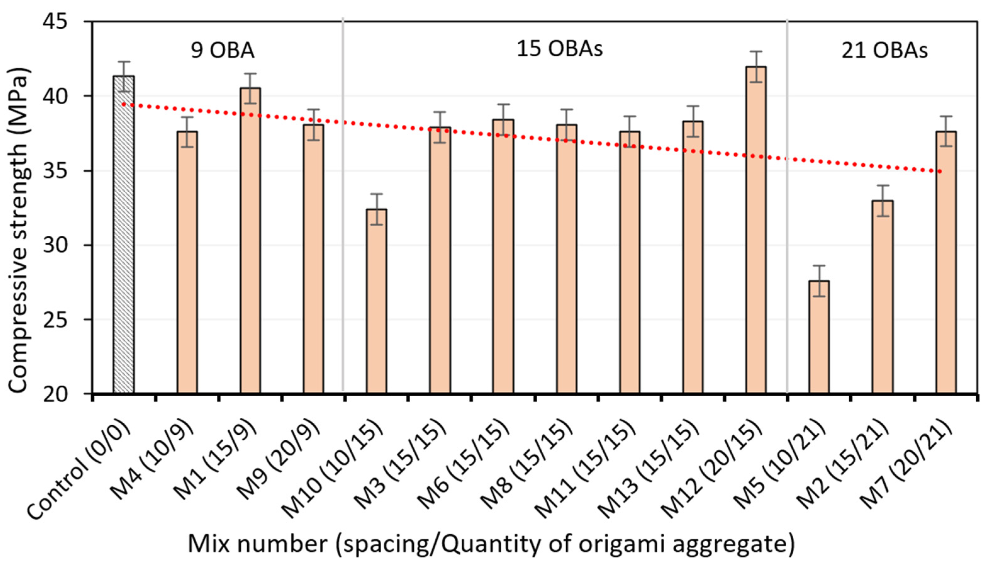
3.2. Compressive Strength of OBA-RECC

The compressive strength of the OBA-REC mixes is shown in Figure 7. The strengths of all the mixes range between 27.58 MPa (M5) and 41.97 MPa (M12). The trend shows a decreasing compressive strength with an increasing quantity of OBA. Some factors attributable to this are the lower strength of the OBA compared to the surrounding hardened cement matrix and the nature of stress distribution of the OBA under load. The stress concentration at the tips of the spikes on the OBA’s surface is responsible for the development and propagation of cracks, which is more noticeable at lower spacings. This explains why the strength increased as the OBA’s spacing increased across all groups. The strength increased from 37.6 MPa at 10 mm spacing (M4) to 40.51 MPa at 15 mm spacing (M1) in the 9 OBA group. In the same vein, the strength increased from 32.4 MPa at 10 mm spacing (M10) to an average of 38 MPa at 15 mm spacing (M3, M6, M8, M11, and M13—the RSM repeated central point mixes) and 42 MPa at 20 mm spacing in the 15 OBA group. A similar trend was observed in the 21 OBA group. Hence, the strength of the mixes was improved by a more uniform stress distribution within the composite at higher OBA spacings.

Furthermore, the tendency of the mix to be well-compacted is higher at wider OBA spacing than when the aggregates are relatively more congested. This led to a more compact and denser ECC at a hardened state with enhanced strength due to better stress transfer between the aggregates and the composite at the interfacial transition zone (ITZ).

Figure 8 shows the failure pattern of the OBA-ECC. As the load increased, the OBA’s deformation and stress concentration caused longitudinal cracks to form along the specimen, as seen in Figure 8a, which eventually caused the concrete’s surface to be removed, as seen in Figure 8b, revealing the OBA. Figure 8c,d show that the specimen had a strong bond between the OBA and the matrix at the ITZ despite the OBA breaking. Hence it is evident that the bubble aggregates contributed to the stress transfer before they failed, as explained by Yan et al. [4], which agrees with the compressive strength result at wider OBA spacings. The OBA outperformed the hollow ceramic and plastic aggregates employed in earlier research in terms of strength [3]. As a result, they could still transfer some stress even after breaking under load, which improved their performance. Additionally, compared to the concave, spherical, or capsule-shaped bubble aggregates employed in earlier experiments, which all had smooth surfaces, there was more physical interlocking and bonding at the interface because of their rough surface and spiky appearance. Additionally, some of the hollow bubble aggregates previously employed had their surfaces modified to improve the bonding with the cement matrix [3,4]. While the bonding improved, their performance suffered because their thin hollow shell was easily deformed under stress, unlike the OBA.

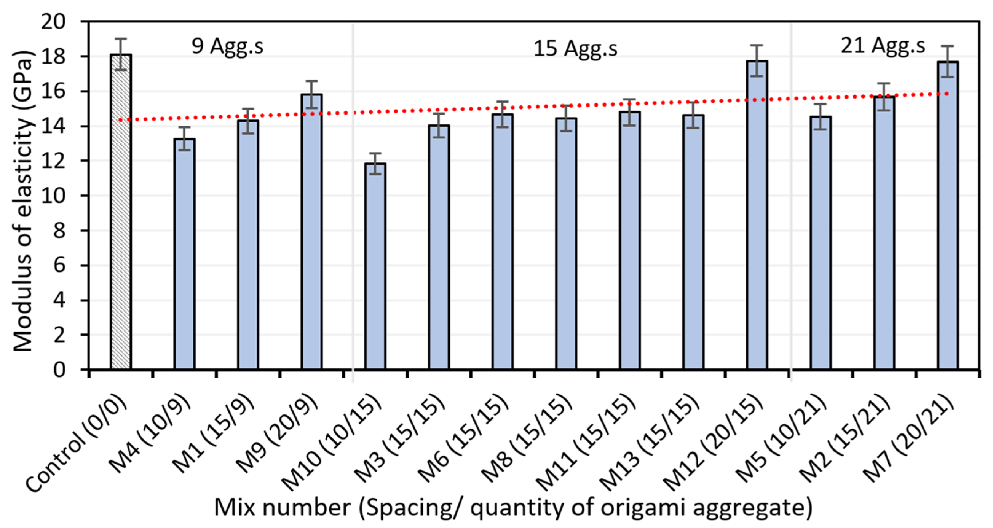
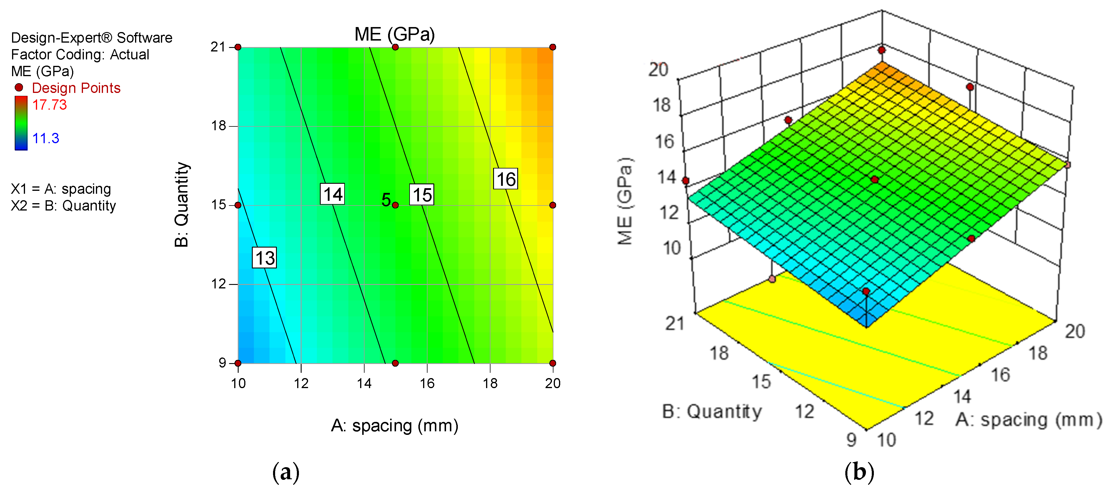
3.3. Modulus of Elasticity and Poisson’s Ratio of OBA-RECC

Figure 9 shows the modulus of elasticity of the OBA-RECC mixes at 28 days. The findings indicate that the mixes’ elastic modulus decreased when the OBA was added. However, the decrease in the elastic modulus was more severe at smaller spacings. The modulus of elasticity values range between 11.83 GPa and 17.69 GPa, representing 34.6% and 2.3% reductions, respectively, compared to the control mix. ECC is known to possess a lower modulus of elasticity than concrete due to the absence of coarse aggregate. Also, the low modulus of elasticity of the ECC is shown to be aggravated by the inclusion of CR [28]. Therefore, even while the addition of OBA caused a substantial decrease in the elasticity of RECC, it is still not as severe as the effects of other types of bubble aggregates on concrete, which were found to reduce the elastic modulus by up to 15.2% to 42.8 [4].

Furthermore, it can be observed that with an increase in the spacing of the OBA, the decrease in the elastic modulus of the mixes was lower. In the 9 OBA group, there is a 10.7% increase in the elastic modulus between M4 (10 mm spacing) and M9 (15 mm spacing). Similarly, there was an increase of 49.87% and 21.83% between a mix with 10 mm spacing and that with 15 mm spacing at both 15 OBA and 21 OBA groups, respectively. The superior stress distribution by the OBA inside the composite compared to when they are closer is the cause of the mixes’ improved elastic modulus at wider spacings. As the space reduced, the stress concentration increased, causing cracks to form and a corresponding decrease in elastic modulus. In addition, when the OBAs get closer, it is harder to produce proper compaction during mixing, which results in a weak composite surrounding the aggregates.

Figure 10 illustrates how, after the addition of 9 OBAs, the Poisson’s ratio (ν) of the OBA-RECC mixes dropped, and after the addition of 15 and 21 OBAs, it increased more than the control. Poisson’s ratio is the ratio of the lateral deformation to the longitudinal deformation. The result showed that the OBA acted like defects inside the composite leading to more deformation of the RECC as the aggregates increased. At 9 OBA, the specimen was better compacted than when the aggregate volume increased, leading to enhanced composite stiffness. However, as the OBA increased to 15 and 21, the composite stiffness drastically reduced, leading to more deformation that translated to higher ν values. However, it is worth noting that in line with the previous discussions on the strength and modulus of elasticity of the OBA-RECC, as the spacing increased, the OBA performed much better in terms of stress distribution leading to the enhancement in the strength and stiffness of the RECC as reflected in the reduced ν values with increased spacings of the OBA. All the mixes’ v values range from 0.22 to 0.31, higher than the range for typical concrete, which is 0.1 to 0.2. This is logical given the impact of CR in the mix, which has a high v value of about 5, as well as the influence of the OBAs.

4. RSM Analysis

4.1. Model Development and ANOVA

The response surface models are developed using linear or quadratic optimal predictive models, whose general forms are presented in Equations (1) and (2) for linear and higher-order polynomials, respectively.

$$y={\beta }_0+{\beta }_1{x}_2+{\beta }_2{x}_2+{\beta }_n{x}_n+ϵ$$

(1)

$$y=\beta {\beta }_0+{\displaystyle \sum }_{i=1}^k{\beta }_i{x}_i+{\displaystyle \sum }_{i=1}^k{\beta }_{ii}{x}_i^2+{\displaystyle \sum }_{j=2}^k{\displaystyle \sum }_{i=1}^{j=1}{\beta }_{ij}{x}_i{x}_j+\epsilon$$

(2)

where $y$ is the response of interest, i and j are, respectively, the linear and quadratic coefficients, $\beta$ represents the regression coefficient, k stands for the number of factors studied and optimized, and $\epsilon$ represents the random error.

Based on the empirical data generated and entered into the RSM tool of design Expert software (version 10), the predictive response models were generated as shown in Equations (3)–(6). In this case, the responses, which are the dependent variables, are the density (D), the compressive strength (CS), the modulus of elasticity (ME), and the Poisson’s ratio (PR). The independent variables are the input factors represented as A and B for the spacing and quantity of the OBA, respectively. Based on the chosen sequential model sum of squares (SMSS), a quadratic model was found more suitable for the density and compressive strength, while the modulus of elasticity and Poisson’s ratio were fitted with linear models.

$$\mathrm{D}=+1948.66-5.83\times \mathrm{A}-10.67\times \mathrm{B}+17.25\times \mathrm{AB}+11.29\times {\mathrm{A}}^2-25.79\times {\mathrm{B}}^2$$

(3)

$$\begin{array}{cc}\mathrm{CS}=+37.88 +& 4.62\times \mathrm{A}-4.27\times \mathrm{B}+0.49\times \mathrm{AB}-0.26\times {\mathrm{A}}^2\\ & -0.71\times {\mathrm{B}}^2\end{array}$$

(4)

$$\mathrm{ME}=+14.70+1.77\times \mathrm{A}+0.59\times \mathrm{B}$$

(5)

$$\mathrm{PR}=+0.27-0.012\times \mathrm{A}-0.035\times \mathrm{B}$$

(6)

ANOVA was performed on the developed models at a 95% confidence interval. Hence all the factors that significantly affect the responses have a probability of less than 5%. Similarly, all the models with a probability of less than 5% are significant. The ANOVA result is shown in

Table 3. ANOVA result.

Response	Source	Sum of Squares	Df	Mean Square	F-Value	p-Value > F	Significance
Density (kg/m3)	Model	5355.5	5	1071.1	23.16	0.0003	YES
	A-Spacing	204.17	1	204.17	4.41	0.0737	NO
	B-Quantity	682.67	1	682.67	14.76	0.0064	YES
	AB	1190.25	1	1190.25	25.74	0.0014	YES
	A2	352.24	1	352.24	7.62	0.0281	YES
	B2	1837.45	1	1837.45	39.73	0.0004	YES
	Residual	323.73	7	46.25
	Lack of fit	262.93	3	87.64	5.77	0.0618	NO
	Pure error	60.8	4	15.2
	Cor Total	5679.23	12
Compressive strength (MPa)	Model	240.57	5	48.11	147.38	<0.0001	YES
	A-Spacing	128.07	1	128.07	392.29	<0.0001	YES
	B-Quantity	109.23	1	109.23	334.58	<0.0001	YES
	AB	0.94	1	0.94	2.88	0.1334	NO
	A2	0.19	1	0.19	0.59	0.4686	NO
	B2	1.41	1	1.41	4.31	0.0766	NO
	Residual	2.29	7	0.33
	Lack of fit	1.88	3	0.63	6.26	0.0543	NO
	Pure error	0.4	4	0.1
	Cor Total	242.85	12
Modulus of elasticity (GPa)	Model	20.8	2	10.4	5.17	0.0287	YES
	A-Spacing	18.73	1	18.73	9.31	0.0122	YES
	B-Quantity	2.08	1	2.08	1.03	0.3336	NO
	Residual	20.12	10	2.01
	Lack of fit	11.51	6	1.92	0.89	0.5726	NO
	Pure error	8.61	4	2.15
	Cor Total	40.93	12
Poisson’s ratio	Model	8.17 × 10−3	2	4.08 × 10−3	22.27	0.0002	YES
	A-Spacing	8.17 × 10−4	1	8.17× 10−4	4.45	0.061	YES
	B-Quantity	7.35 × 10−3	1	7.35 × 10−3	40.09	<0.0001	YES
	Residual	1.83 × 10−3	10	1.83 × 10−4
	Lack of fit	1.55 × 10−3	6	2.59 × 10−4	3.7	0.1131	NO
	Pure error	2.80 × 10−4	4	7.00 × 10−5
	Cor Total	1.00 × 10−2	12

, which reveals that for the density model, B, AB, A², and B² were significant. For the compressive strength model, A and B were the significant model terms, while only A was significant in the modulus of elasticity model. Poisson’s ratio model had A and B as significant model terms. For all the models, the lack of fit is not significant, which is desirable for the models to fit.

The model validation parameters in

Table 4. Model validation parameters.

Parameter	D	CS	ME	PR
Std. Dev.	6.80	0.57	1.42	0.01
Mean	1931.54	37.43	14.70	0.27
CV %	0.35	1.53	9.65	5.01
PRESS	2763.22	16.18	33.97	0.00
−2 Log Likelihood	78.69	14.29	42.57	−78.37
R2	0.94	0.99	0.51	0.82
Adj R2	0.90	0.98	0.41	0.78
Pred R2	0.51	0.93	0.17	0.67
Adeq Precision	12.81	45.79	6.91	14.35
BIC	94.08	29.68	50.27	−70.68
AICc	104.69	40.29	51.24	−69.71

show that all the developed models have a high coefficient of determination (R²) ranging between 51 and 99%. When stated as a percentage or as a range from 0 to 1, the R² demonstrates how well the selected model matches the data. Better model fit is indicated by higher R² values [29]. Consequently, in this instance, all developed models fit the data appropriately. Similarly, for a strong model, the difference between the adjusted and predicted R² should not be more than 0.2, a condition satisfied by all the models in this case. Furthermore, adequate precision is used to measure the signal-to-noise ratio, and a value of more than 0.4 is required. The adequate precision values of the developed models range from 6.91 to 45.79, all satisfying the requirement for adequate signal.

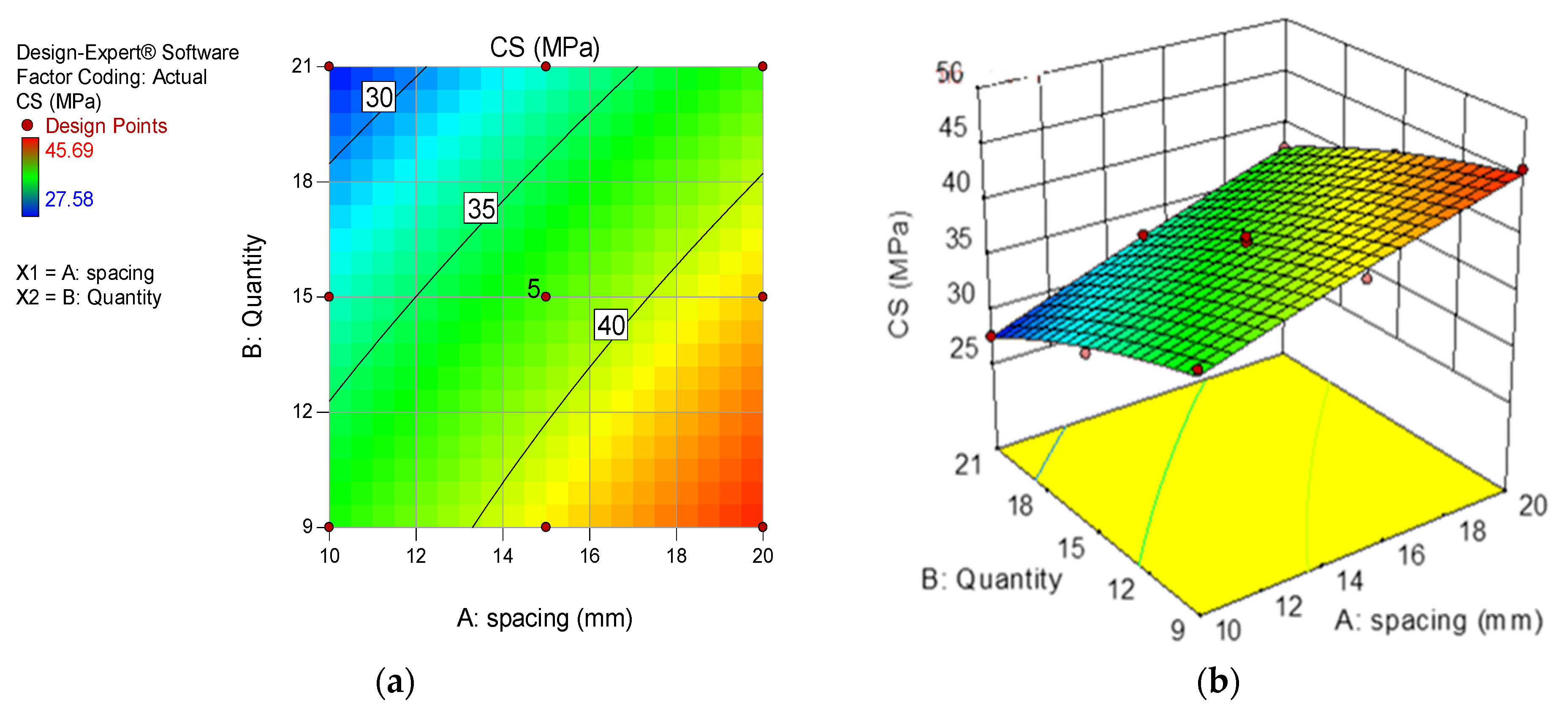
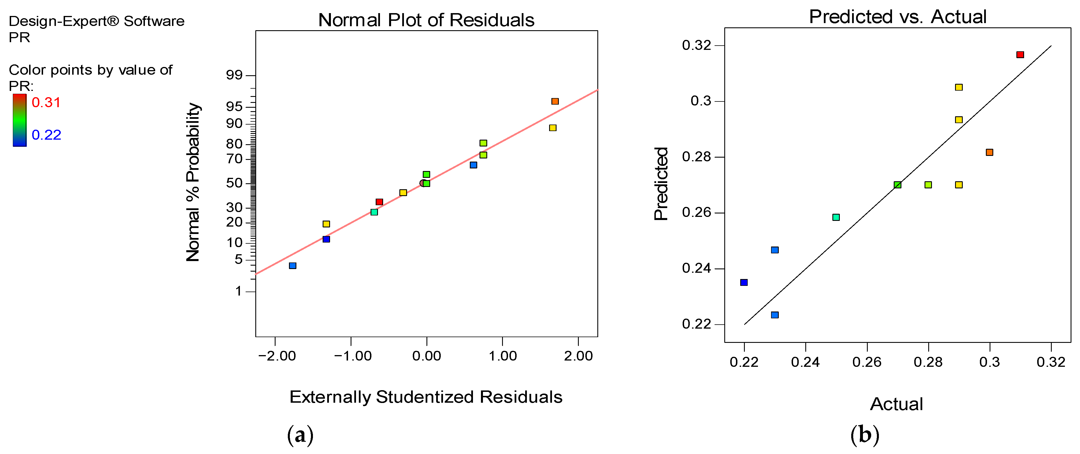
4.2. Model Graphs and Diagnostic Plots

The relationship between the input variables (input factors) and their individual and interaction effect on the dependent variable (response) is represented using 2D contour and 3D response surface diagrams. These graphs show how the levels of the independent variables affect the response through a color gradient. The 2D plot expresses the interaction of the variables using contours that show varying response levels at particular levels of the input factors. On the other hand, the 3D response surface diagrams show the same information as the 2D but in a 3D format, as the name implies. The 2D contour and 3D response surface diagrams for the developed response models are presented in Figure 11, Figure 12, Figure 13 and Figure 14. The highest levels of the responses are shown in the red regions of the plots, while the blue regions indicate the lowest levels. The yellow and green regions of the plots represent the intermediate levels of the responses.

By observing these model graphs, it can be noticed that the effect of the input factors (spacings and quantities of OBA) on the responses directly corresponds with the discussions in previous sections. For example, the drop in the contours in the 2D plot and the steady decline from the peak in the 3D response surface diagram in Figure 11a,b, respectively, show how the density of the mixes significantly reduced as the quantity and spacings of the OBA increased. There is a move from the red region to the blue region on the graphs. Hence, since it is desired for the OBA-RECC to have low density, higher OBA quantities of 18 to 21 should be used at spacings of 18–20 mm to obtain intermediate to lowest densities (below 1940 kg/m³). Similarly, to develop an OBA-RECC with high strength (above 40 MPa) within the range of strength values obtained during the experiments, 9–15 OBA should be used at spacings of 16 to 20 mm, as shown in Figure 12. Similar interpretations can be made for the other model graphs.

Other very important graphs in the RSM analysis are the model diagnostic plots, such as the normal plot of residuals and the actual versus predicted plot. The normal residual plot is used to check whether the residuals (error terms) are normally distributed, a condition required for the model’s reliability. This is assessed by the linearity of the data points along the diagonal straight line representing the ideal normal distribution. Hence, as shown in the (a) part of Figure 15, Figure 16, Figure 17 and Figure 18, all the developed models have linearly aligned residuals signifying that the error terms are normally distributed, and the models are reliable.

Furthermore, the actual versus predicted plot visually assesses the model fit and shows the variation resulting from random effects. The distribution of the points along a regression line is used to evaluate the correlation between the observed and predicted values, shown in the scatter plot. The closeness of the data points to the diagonal line indicates how high the coefficient of determination of the models is. Also, for a perfect fit model, the distribution of the points should be uniform along the straight line. Any skewness in the data will be indicated by the points being more on one side of the diagonal line. As shown in the (b) part of Figure 15, Figure 16, Figure 17 and Figure 18, all the developed models have a good fit, further confirming the models’ strength and adequacy for response prediction purposes.

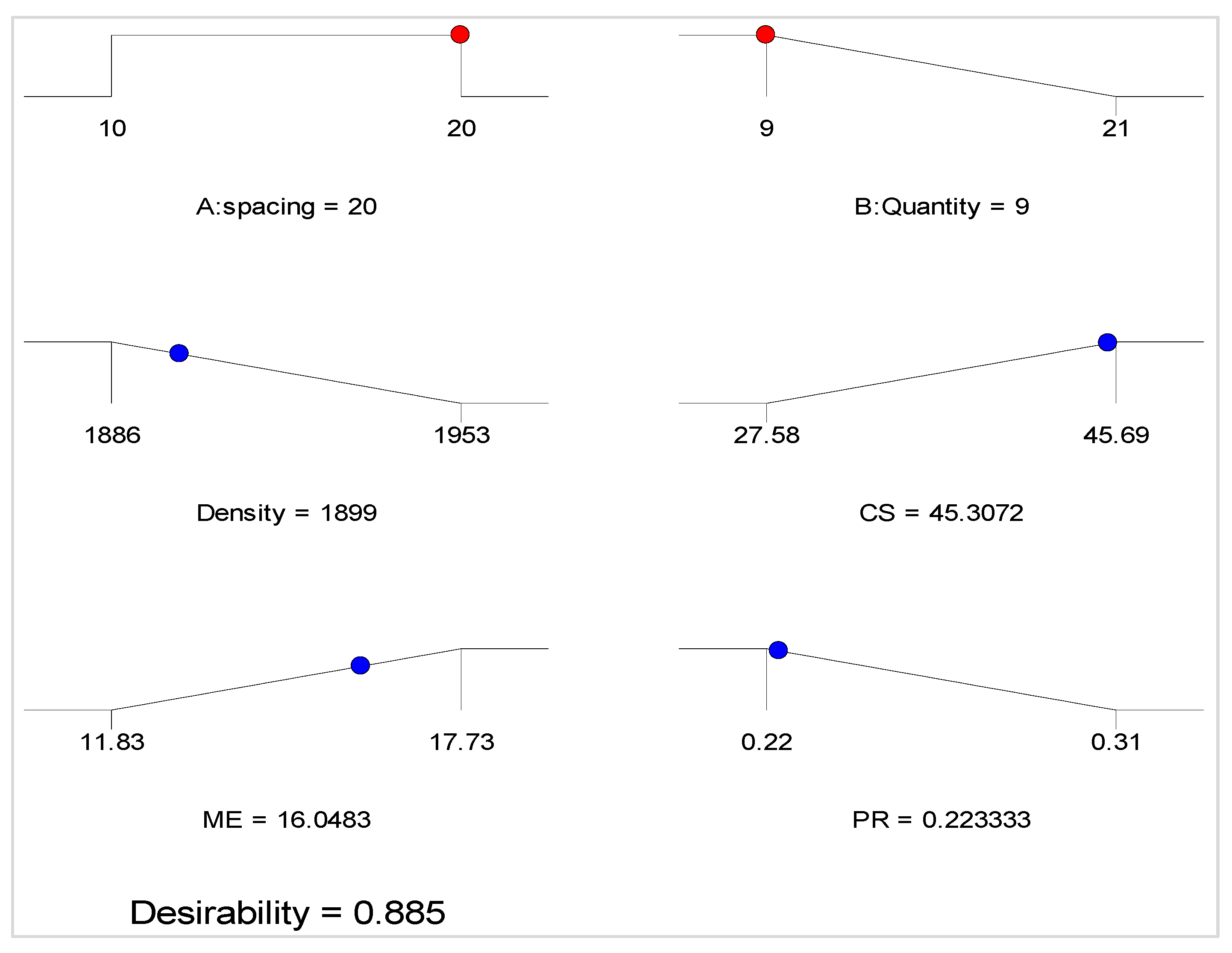
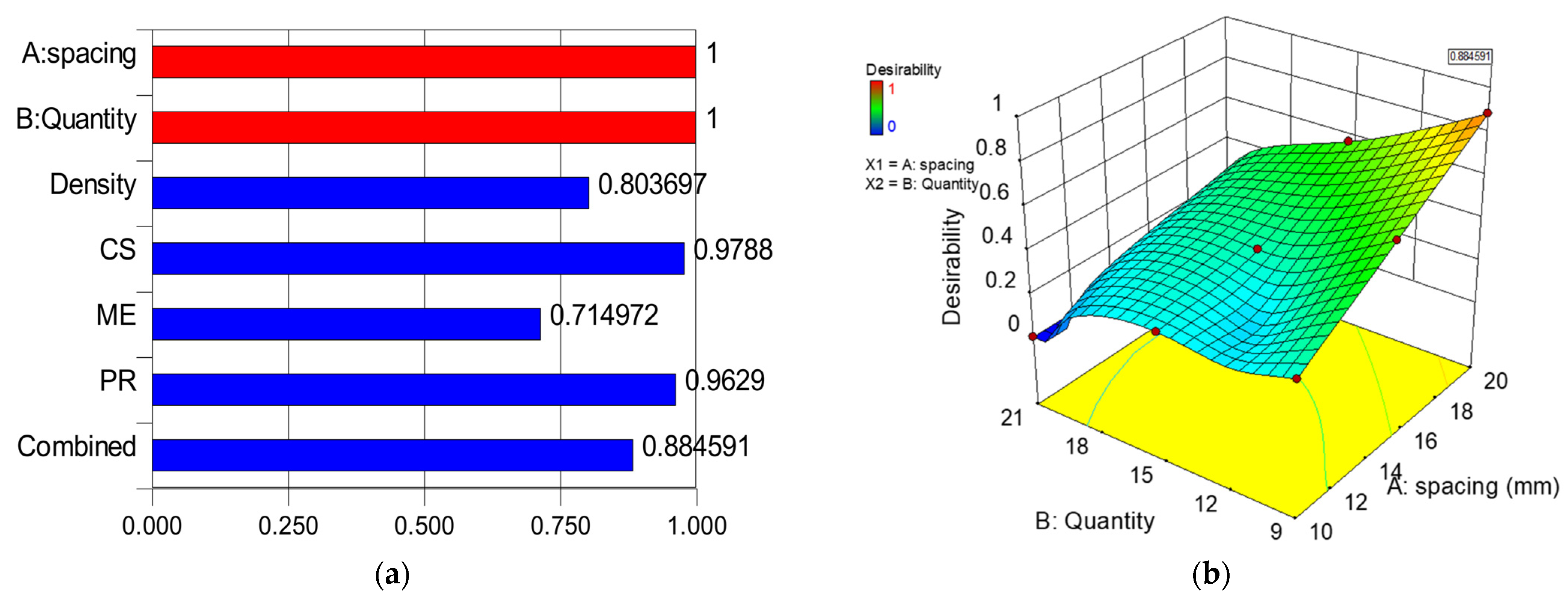
4.3. Multi-Objective Optimization

Multi-objective optimization is a branch of multiple-criteria decision-making that deals with mathematical optimization problems where multiple objective functions must be simultaneously optimized [30]. This approach is recommended because most real-world optimization problems involve identifying many best solutions among many competing objectives. In order to achieve the objective functions without compromising the responses, goals are specified for the independent and dependent variables with varied criteria and levels of priority. The desirability value d_j, with a range of values defined as 0 ≤ d_j ≤ 1, is used to evaluate the optimization result, as shown in Equation (7). The better the outcome, the greater the d_j value (given as a percentage).

$$D={\left(d_1^{r_1}\times d_2^{r_2}\times d_3^{r_3}\times \dots \times d_n^{r_n}\right)}^{\raisebox{1ex}{$1$}\!\left/ \!\raisebox{-1ex}{$n$}\right.}$$

(7)

where n is the number of responses taken into account during optimization, and rⁱ denotes the significance of each objective function d_i on a scale from one (least important) to five (most important).

The objective functions for the input and output variables are shown in

Table 5. Objective functions.

Factors		Unit	Goal	Lower Limit	Upper Limit
Input variables	A: Spacing	mm	In range	10	20
	B: Quantity	-	Minimize	9	21
Responses	D	Kg/m3	Minimize	1886	1953
	CS	MPa	Maximize	27.58	45.69
	ME	GPa	Maximize	11.83	17.73
	PR	-	Minimize	0.22	0.31

. In order to produce the most desirable responses at the lowest OBA feasible, the quantity’s objective was set to minimize the OBA, while the goal for the spacing was set within the range of the values utilized in the experiment. The aim was to produce an ECC with low density; hence the density objective function was minimized. The compressive strength and modulus of elasticity of the composite were maximized, while Poisson’s ratio was minimized. Out of the five levels available, three (the default) was kept as the priority level for all the factors. When the optimization was run, the solution obtained is presented in Figure 19 in the form of ramps. Out of the nine solutions provided by the RSM, the first one was chosen. The optimal input factors were 20 mm spacing and 9 OBAs, which will produce optimum D, CS, ME, and PR of 1899 Kg/m³, 45.3 MPa, 16.05 GPa, and 0.22, respectively, at a desirability of 88.5%. Figure 20 shows the individual factors and the combined desirabilities for the optimization.

4.4. Experimental Validation

The final stage of the RSM analysis is to perform an experimental validation of the developed response predictive models. This was achieved by casting RECC using the spacings and quantities obtained from the optimization solution. Three cylinder samples for the density, compressive strength, modulus of elasticity, and Poisson’s ratio determination were cast from the optimum mix. After curing for 28 days, the samples were subjected to various tests accordingly, and the average experimental results obtained are shown together with the predicted results in

Table 6. Experimental validation result.

Response	Experimental Result	Predicted Result	Percentage Error (%)
D (kg/m3)	1781	1899	6.2
CS (MPa)	49.8	45.3	9.9
ME (GPa)	18.2	16.1	8.7
PR	0.21	0.22	4.5

. The error ($\delta$) between each response’s experimental and predicted values was computed using Equation (8). The outcome showed that the two had a good agreement for all properties with $\delta$ value of less than 10%. This demonstrates that the developed response predictive models are reliable and accurate.

$$\delta =\left|\frac{{\vartheta }_E-{\vartheta }_P}{{\vartheta }_P}\right|\times 100\%$$

(8)

5. Conclusions

At the end of the research, the following conclusions were drawn:

• Using origami bubble aggregate (OBA) to produce a lightweight ECC is a novel approach, and an RECC with a density of 1781 kg/m³ can be produced, with a 20% lower density than the control RECC.
• Compared to other hollow bodies employed in earlier studies, RECC with significant compressive strength can be produced using 15 OBAs at spacings between 15 and 20 mm.
• At all OBA quantities, the modulus of elasticity was higher at higher OBA spacings, which were close to the values of the control RECC mix. On the other hand, lower Poisson’s ratios than control RECC were obtained at a quantity of 9 OBA at all the spacings under consideration. Nevertheless, the trend changed with higher OBA quantities, with the highest ME values obtained at lower spacings.
• Predictive response models were developed and validated using ANOVA with high R² ranging between 51 and 99%. In order to obtain the levels of the input factors that will yield the best performance, multi-objective optimization was performed, which produced optimal input factors of 20 mm and 9 OBAs that will give the optimum density, compressive strength, modulus of elasticity, and Poisson’s ratio of 1899 kg/m³, 45.3 MPa, 16.1 GPa, and 0.22, respectively, at a very high desirability value of 88.5%. Experimental validation showed very good agreement between the experimental and predicted response values at an acceptable error of less than 10% for all the models.
• This research focused on the density reduction effect of OBAs on ECC and the consequent effect on the compressive strength, modulus of elasticity, and Poisson’s ratio of the composite. Other properties of the OBA-RECC not covered here are presently being investigated.

References

1. Chen, Z.; Li, J.; Yang, E.-H. Development of Ultra-Lightweight and High Strength Engineered Cementitious Composites. J. Compos. Sci. 2021, 5, 113. [Google Scholar] [CrossRef]
2. Somasundaram, S.; Ramasamy, K.A.; Mallika, G.S. Development of light weight engineered cementitious composites. In Proceedings of the 3rd National Conference on Current and Emerging Process Technologies CONFEST 2020, Erode, India, 25 January 2020. [Google Scholar] [CrossRef]
3. Yan, X.; Chen, P.S.; Al-Fakih, A.; Liu, B.; Mohammed, B.S.; Jin, J. Experiments and Mechanical Simulation on Bubble Concrete: Studies on the Effects of Shape and Position of Hollow Bodies Mixed in Concrete. Crystals 2021, 11, 858. [Google Scholar] [CrossRef]
4. Yan XChen, P.S.; Liu, B.; Mohammed, B.S.; Jin, J. Effect of Hollow Body Material on Mechanical Properties of Bubble Concrete. Crystals 2022, 12, 708. [Google Scholar] [CrossRef]
5. Chen, P.S.; Tsukinaga, Y. Basic research on the development of light weight concrete mixed with hollow spheres. J. Soc. Mater. Sci. Jpn. 2015, 64, 711–717. [Google Scholar] [CrossRef] [Green Version]
6. Chen, P.S. Bubble Concrete; Japan Patent Office: Tokyo, Japan, 2008. [Google Scholar]
7. Chen, P.S. A study report on light weight concrete mixed with high strength hollow bubbles. In Proceeding of the AIJ Tohoku Chapter Architectural Research Meeting (Kouzoukei); Architectural Institute of Japan: Tokyo, Japan, 2008. [Google Scholar] [CrossRef]
8. Yan, X.; Chen, P.S.; Liu, B.; Mohammed, B.S.; Jin, J. Effect of Hollow Bodies on the Strength and Density of Bubble Concrete. In Proceedings of the AWAM International Conference in Civil Engineering (AICCE’22), Penang, Malaysia, 21–22 August 2022. [Google Scholar]
9. Mohammed, B.S.; Achara, B.E.; Nuruddin, M.F.; Yaw, M.; Zulkefli, M.Z. Properties of nano-silica-modified self-compacting engineered cementitious composites. J. Clean. Prod. 2017, 162, 1225–1238. [Google Scholar] [CrossRef]
10. Li, V.C. Engineered Cementitious Composites (ECC)—Material, Structural, and Durability Performance. In Concrete Construction Engineering Handbook, Nawy, E., Ed.; CRC Press: Boca Raton, FL, USA, 2008; Available online: https://tinyurl.com/ycxdsnby (accessed on 23 October 2022).
11. Li, V.C. Damage Tolerant ECC for Integrity of Structures Under Extreme Loads. In Structures Congress 2009; ASCE: Ausin, TX, USA, 2009. [Google Scholar] [CrossRef] [Green Version]
12. Lepech, M.D.; Li, V.C.; Robertson, R.E.; Keoleian, G.A. Design of Green Engineered Cementitious Composites for Improved Sustainability. ACI Mater. J. 2008, 105, 567. [Google Scholar]
13. Lye, H.L.; Mohammed, B.S.; Liew, M.S.; Wahab, M.M.A.; Al-fakih, A. Bond behaviour of CFRP-strengthened ECC using Response Surface Methodology (RSM). Case Stud. Constr. Mater. 2020, 12, e00327. [Google Scholar] [CrossRef]
14. Zhang, Z.; Zhang, Q. Matrix tailoring of Engineered Cementitious Composites (ECC) with non-oil-coated, low tensile strength PVA fiber. Constr. Build. Mater. 2018, 161, 420–431. [Google Scholar] [CrossRef]
15. Abdulkadir, I.; Mohammed, B.S.; Liew, M.S.; Wahab, M.M.A.; Zawawi, N.A.W.A.; As’ad, S. A review of the effect of waste tire rubber on the properties of ECC. Intern. J. Adv. Appl. Sci. 2020, 7, 105–116. [Google Scholar]
16. Abdulkadir, I.; Mohammed, B.S.; Liew, M.S.; Wahab, M.M.A. Modelling and multi-objective optimization of the fresh and mechanical properties of self-compacting high volume fly ash ECC (HVFA-ECC) using response surface methodology (RSM). Case Stud. Constr. Mater. 2021, 14, e00525. [Google Scholar] [CrossRef]
17. Zhang, Z.; Yuvaraj ADi, J.; Qian, S. Matrix design of light weight, high strength, high ductility ECC. Constr. Build. Mater. 2019, 210, 188–197. [Google Scholar] [CrossRef]
18. Wang, S.; Li, V. Lightweight engineered cementitious composites (ECC). In Proceedings of the 4th International RILEM Workshop on High Performance Fiber Reinforced Cement Composites (HPFRCC 4), Ann Arbor, MI, USA, 16–18 June 2003; RILEM Publications: Paris, France, 2003. [Google Scholar]
19. Huang, X.; Ranade, R.; Zhang, Q.; Ni, W.; Li, V.C. Mechanical and thermal properties of green lightweight engineered cementitious composites. Constr. Build. Mater. 2013, 48, 954–960. [Google Scholar] [CrossRef]
20. Singh, S.B.; Munjal, P. Engineered cementitious composite and its applications. Mater. Today Proc. 2020, 32, 797–802. [Google Scholar] [CrossRef]
21. Li, V.C. On engineered cementitious composites (ECC) a review of the material and its applications. J. Adv. Concr. Technol. 2003, 1, 215–230. [Google Scholar] [CrossRef] [Green Version]
22. Mohammed, B.S.; Nuruddin, M.F.; Aswin, M.; Mahamood, N.; Al-Mattarneh, H. Structural Behavior of Reinforced Self-Compacted Engineered Cementitious Composite Beams. Adv. Mater. Sci. Eng. 2016, 2016, 5615124. [Google Scholar] [CrossRef] [Green Version]
23. Mohammed, B.S.; Yen, L.Y.; Haruna, S.; Seng Huat, M.L.; Abdulkadir, I.; Al-Fakih, A.; Liew, M.S.; Zawawi, N.A.W.A. Effect of Elevated Temperature on the Compressive Strength and Durability Properties of Crumb Rubber Engineered Cementitious Composite. Materials 2020, 13, 3516. [Google Scholar] [CrossRef] [PubMed]
24. Abdulkadir, I.; Mohammed, B.S.; Ali, M.O.A.; Liew, M.S. Effects of Graphene Oxide and Crumb Rubber on the Fresh Properties of Self-Compacting Engineered Cementitious Composite Using Response Surface Methodology. Materials 2022, 15, 2519. [Google Scholar] [CrossRef] [PubMed]
25. Mohammed, B.S.; Achara, B.E.; Liew, M.S.; Alaloul, W.S.; Khed, V.C. Effects of elevated temperature on the tensile properties of NS-modified self-consolidating engineered cementitious composites and property optimization using response surface methodology (RSM). Constr. Build. Mater. 2019, 206, 449–469. [Google Scholar] [CrossRef]
26. BS EN 12390-7:2000; Testing Hardened Concrete. British Standards: London, UK, 2000.
27. ASTM C 39/C 39M-01; Standard Test Method for Compressive Strength of Cylindrical Concrete Specimens. ASTM: West Conshohocken, PA, USA, 2001.
28. Mohammed, B.S.; Xian, L.W.; Haruna, S.; Liew, M.S.; Abdulkadir, I.; Zawawi, N.A.W.A. Deformation Properties of Rubberized Engineered Cementitious Composites Using Response Surface Methodology. Iran. J. Sci. Technol. Trans. Civ. Eng. 2021, 45, 729–740. [Google Scholar] [CrossRef]
29. Khed, V.C.; Mohammed, B.S.; Zawawi, N.A.W.A. Development of response surface models for self-compacting hybrid fibre reinforced rubberized cementitious composite. Constr. Build. Mater. 2020, 232, 117191. [Google Scholar] [CrossRef]
30. Deb, K. Multi-Objective Optimization. In Search Methodologies: Introductory Tutorials in Optimization and Decision Support Techniques, Burke, E.K., Kendall, G., Eds.; Springer: New York, NY, USA; Heidelberg, Germany; Dordrecht, The Netherlands; London, UK, 2014. [Google Scholar]
Figure 1. Different types of bubble aggregates: (a) Hollow spheres with surface treatment; (b) Reinforced spheres; (c) Concave bubbles.
Buildings 12 02201 g001
Figure 2. (a) Origami bubble aggregate (OBA); (b) Kusudama origami that inspired the OBA.
Buildings 12 02201 g002
Figure 3. (a) A schematic diagram of the OBA showing its dimensions; (b) The 3D printed OBAs.
Buildings 12 02201 g003
Figure 4. (a) Origami aggregate before casting; (b) Schematics of the 9, 15, and 21 OBAs inside the cylinder at 20 mm spacings.
Buildings 12 02201 g004
Figure 5. (a) Compressive strength test; (b) Modulus of elasticity and Poisson’s ratio test.
Buildings 12 02201 g005
Figure 6. The density of OBA-RECC mixes.
Buildings 12 02201 g006
Figure 7. Compressive strength of OBA-RECC mixes at 28 days.
Buildings 12 02201 g007
Figure 8. Failure pattern of OBA-RECC (a) Longitudinal cracks on the sample (b) larger sample cracks at a higher load (c) and (d) Failed samples showing a good bonding between the OBA and the hardened matrix.
Buildings 12 02201 g008
Figure 9. The modulus of elasticity of OBA-RECC mixes at 28 days.
Buildings 12 02201 g009
Figure 10. Poisson’s ratio of OBA-RECC mixes at 28 days.
Buildings 12 02201 g010
Figure 11. (a) Two-dimensional contour plot; (b) Three-dimensional response surface diagram for D model.
Buildings 12 02201 g011
Figure 12. (a) Two-dimensional contour plot; (b) Three-dimensional response surface diagram for CS model.
Buildings 12 02201 g012
Figure 13. (a) Two-dimensional contour plot; (b) Three-dimensional response surface diagram for ME model.
Buildings 12 02201 g013
Figure 14. (a) Two-dimensional contour plot; (b) Three-dimensional response surface diagram for PR model.
Buildings 12 02201 g014
Figure 15. (a) The normal plot of residuals and (b) actual versus predicted plot for the OBA-RECC D model.
Buildings 12 02201 g015
Figure 16. (a) The normal plot of residuals and (b) actual versus predicted plot for the OBA-RECC CS model.
Buildings 12 02201 g016
Figure 17. (a) The normal plot of residuals and (b) actual versus predicted plot for the OBA-RECC ME model.
Buildings 12 02201 g017
Figure 18. (a) The normal plot of residuals and (b) actual versus predicted plot for the OBA-RECC PR model.
Buildings 12 02201 g018
Figure 19. Optimization solution ramps.
Buildings 12 02201 g019
Figure 20. (a) Desirability value of individual factors; (b) Three-dimensional response surface diagram of the combined desirability of the optimization.
Buildings 12 02201 g020