

Thermal Bridge Modeling According to Time-Varying Indoor Temperature for Dynamic Building Energy Simulation Using System Identification


1
Institute of Construction and Environmental Engineering, Seoul National University, Seoul 08826, Republic of Korea
2
Department of Architectural Engineering, College of Engineering, Kwangwoon University, Seoul 01897, Republic of Korea
3
Department of Architecture and Architectural Engineering, College of Engineering, Seoul National University, Seoul 08826, Republic of Korea
*
Author to whom correspondence should be addressed.
Buildings 2022, 12(12), 2178; https://doi.org/10.3390/buildings12122178
Submission received: 20 July 2022
/
Revised: 24 October 2022
/
Accepted: 29 November 2022
/
Published: 8 December 2022
(This article belongs to the Section Building Energy, Physics, Environment, and Systems)
Abstract
:It is not easy to dynamically analyze thermal bridges that require multi-dimensional analysis in building energy simulations, which are mostly one-dimensional platforms. To solve this problem, many studies have been conducted and, recently, a study was conducted to model a thermal bridge based on the data obtained by approaching this in a similar way to steady-state analysis, showing high accuracy. This was an early-stage study, which is only applicable when the indoor temperature is constant. By extending the study, a thermal bridge model that can be applied even when the indoor temperature changes over time in building energy simulations is proposed and validated. Since the governing equation, the heat diffusion equation, is linear, the key idea is to create and apply two thermal bridge transfer function models by expressing the heat flow that enters the room as a linear combination of the transfer function for indoor temperature and the transfer function for outdoor temperature. For the proposed thermal bridge model, the NRMSE of the model itself showed a high accuracy of 0.001, and in the verification through annual simulation using the model, the NRMSE showed an accuracy of 0.1.
1. Introduction
We live in an era of high oil prices and are facing energy problems. Efforts are being made in terms of energy supply to find various sources of renewable energy, such as solar power and fuel cells, to replace the existing fossil fuels that cause environmental problems, such as greenhouse gases and fine dust. In addition, research on energy reductions in terms of energy demand is also essential for solving energy problems. Almost all fields are concerned with the issue of energy reduction, and agree that sustainable development is possible with minimal energy consumption.
A building, a space where humans live, must be kept in a comfortable state and protected from external environments, such as cold and hot environments, and energy required for heating and cooling is consumed to maintain this. The energy required for a building may increase or decrease depending on the architectural design and materials used in the building [1,2,3]. In the field of building energy engineering, research on energy reduction technology for each building element, such as the building envelope and window system, is being conducted [4,5,6]. The building envelope is the part that is in direct contact with the external environment; minimizing heat flow through the building envelope is one of the key factors in reducing building energy [7].
Meanwhile, to develop and evaluate building energy reduction technology, experimental methods and computer simulation methods are used. Although the experimental method of constructing a building for each building element or experimental mock-up test is important, the computer simulation method is used because the experimental building scale is large and it is not easy to experiment with various methods under various conditions. Therefore, building energy simulation (BES) programs that can explain various physical phenomena related to buildings are widely used in building energy engineering [8,9,10].
In the BES, numerous architectural elements, such as building envelopes and windows, and building equipment, such as HVAC systems, are modeled, and the complex heat-transfer phenomenon that occurs in each component is dynamically calculated to analyze the building energy. In addition, since the simulation period is usually one year, the BES is computationally demanding and takes a significant amount of time [11]. For this reason, the model for each BES component should be simple, uncomplicated, and have low computational complexity.
To analyze the building envelope, it is necessary to analyze the convection and radiation that occur on the surface of the building envelope, as well as the conduction that occurs inside the building envelope. This heat-transfer phenomenon is expressed as a heat diffusion equation, which is a three-dimensional dynamic equation. To solve this heat diffusion equation in the BES, it is simplified with a one-dimensional assumption. This assumption is reasonable in that the building envelope is usually composed of several material layers, which are arranged one-dimensionally. However, this assumption is not suitable for complex geometries that are difficult to analyze in one dimension because the materials are broken, for example, the so-called thermal bridges [12,13,14].
A thermal bridge (TB) is the part of the building envelope where the insulation is broken, and the thermal performance is weak. Many studies have pointed out the energy loss caused by TBs [15,16,17,18], and technological developments, such as thermal breakers, have been developed as a solution to TBs [19,20,21]. In addition, various modeling and analysis methods for TBs in BES have been developed [12].
Most BES programs, such as EnergyPlus [22] and TRNSYS [23], do not analyze TBs that require multi-dimensional analysis because they are one-dimensional platforms. When the evaluation of TBs is considered in BES, the method of adding the steady-state TB analysis results to the BES results is used, with the linear thermal transmittance reflecting the effect of TBs in the steady state. In addition to these methods, various methods, such as the structure factors method [24], the matrix of transfer functions method [25], the one harmonic method [26], and the identification method [27], have been proposed. However, although, theoretically, many methods have been proposed, they have not been applied to BES because they are not simple enough.
Thermal bridge modeling and the dynamic analysis method have been proposed using the analogy of a steady-state thermal bridge analysis [28]. This method started from the relatively widely used steady-state analysis method for TBs, and is easy to access, as it is a data-driven method that has been widely used in many academic fields. The most important aspect is the separation of the time-series heat-flow data that enter the room through the wall into the time-series heat-flow data that enter the room through the wall and can be analyzed in one dimension (the clear wall), and the time-series heat-flow data that enter the room through the thermal bridge region (TB region), the remaining region. Here, to create a model that can explain the time-series heat-flow data that enter the room through the TB region, the transfer function of the TB using the data is proposed as a data-driven model. The modeling method that considered the TB as a dynamic system and uses the outdoor temperature as the input and the heat flow as the output has a fairly high accuracy, but has a limitation in that all parameters except input/output are assumed to be constant. The assumption that the indoor temperature is constant is sometimes used to find the size of heating and cooling equipment when the indoor temperature is kept constant at the set temperature, but the actual indoor temperature is not constant and changes with time. For a more accurate building energy simulation, it is necessary to consider the change in indoor temperature over time. Therefore, it is necessary to examine whether the transfer function model is applicable when the indoor temperature changes over time.
The aim of this study is to establish a TB model that can be applied even when the indoor temperature, as well as the outdoor temperature, changes, starting from the TB model in the BES that was studied in a previous study [28]. The method of analyzing the entire wall is divided into the heat flow that enters the room through the wall, which can be analyzed in one dimension, and the rest of the heat flow, as reported in the previous study. The heat flow that enters the room through a one-dimensional analyzable wall can be analyzed by a model such as the conduction transfer function (CTF) or the finite difference method (FDM) based on the first principles (physical laws) and is currently being used in all building energy simulations. For this reason, we focus on a model that can only explain the rest of the heat flow, which is the TB model. This method involves dividing the building envelope by heat flow rather than geometrically dividing the building envelope to account for TB. Therefore, the objective of this study is to establish a TB model from the perspective of heat flow when the indoor temperature changes over time. One of the things to consider in TB model development is the ability to accurately represent the heat flow through the TB when the indoor and outdoor temperatures change over time. This method should be simple and not computationally complex, so that it can be calculated in a building energy simulation program.
2. Methods
2.1. Building Envelope Analysis and Thermal Bridge Modeling Concept
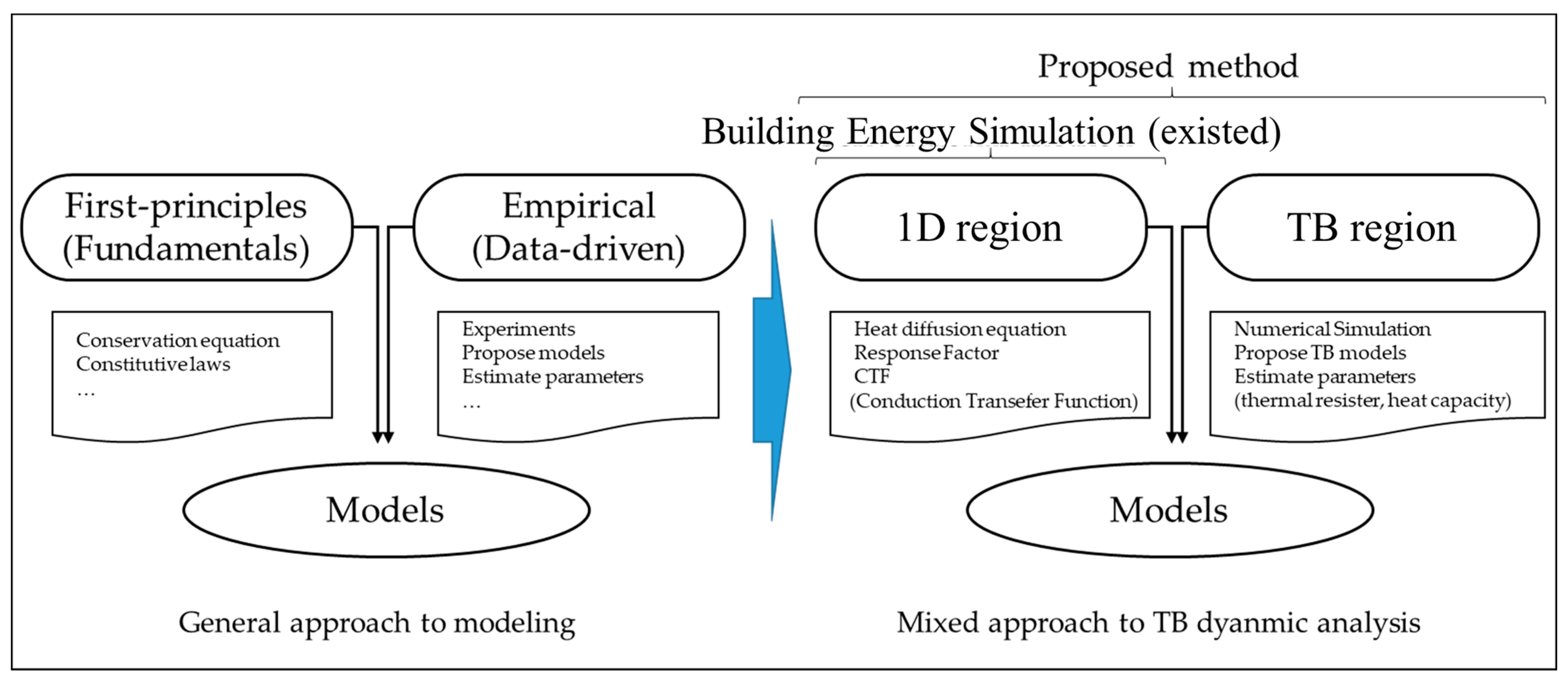
General approaches to modeling include first-principles based on fundamentals and empirical methods based on data [29]. In building envelope analysis, first-principle approach is possible for the region where one-dimensional analysis possible, but TB region is not. Therefore, the modeling concept is established using both approaches. The overall concept for the building envelope analysis and TB modeling in this paper, which is consistent with the previous study [28], is shown in Figure 1. From the perspective of heat flow, the total heat flow that enters the room through the building envelope is divided into the heat flow that enters through the building envelope (the clear wall) that can be analyzed in one dimension, and the heat flow that enters through the building envelope (TB region), which requires multi-dimensional analysis. In order to analyze the building envelope by dividing it in this way, a model is required that can explain the heat flow that enters the room through each path. In this research, the clear wall model uses the first physical law (fundamentals), and the TB region uses an empirical method (data-driven) using data. The model for the clear wall is currently used in most BESs in the form of the FDM [22] or transfer function [22,23]. Therefore, the building envelope can be accurately analyzed by creating a model for the TB region, that is, the TB model and the addition of this to the BES.
2.2. Indoor Temperature and Thermal Bridge Modeling
2.2.1. Indoor Temperature: Constant
In the previous study [28], the TB model was regarded as a linear time invariant system (LTI system), and the modeling method was proposed in the form of a transfer function using system identification, with the outdoor temperature as the input and the heat flow that entered the room through the TB region as the output. The study showed very high accuracy. When analyzing the heating and cooling load to maintain a constant, set indoor temperature, it is correct to assume that the indoor temperature does not change over time, but it is predicted that this method will not be valid when the indoor temperature changes over time. In a dynamic situation, although the indoor temperature changes, assuming that the change is small, it is confirmed that this method is appropriate to some extent. Therefore, in this study, the TB model, the result of the previous study, is applied when the room temperature changes and its effectiveness is validated.
2.2.2. Indoor Temperature: Variable
To model the heat flow that enters the room when the indoor temperature changes over time, it is necessary to check the relation between the heat flow and the indoor temperature with the fundamentals (the laws of physics). The heat transfer phenomenon that occurs in the building envelope is expressed by the heat diffusion equation. The heat diffusion equation is a linear equation, with respect to temperature. Meanwhile, the temperature can be divided into the indoor temperature and the outdoor temperature. Therefore, the heat flow according to each type of temperature can be linearly combined to express the heat flow. By paying attention to the linearity of the governing equation, the TB model can be expressed by dividing it into two models, one for the indoor temperature and one for the outdoor temperature. In the previous study, a TB model for the outdoor temperature was studied using the outdoor temperature as input and the heat flow that entered the room as output. In this study, a TB model for the indoor temperature is studied in a similar way, using the indoor temperature as the input and the heat flow that enters the room as the output. If the output is negative, it means that the heat flow moves from the indoors to the outdoors, normally in the heating season.
The thermal bridge modeling procedure according to the indoor temperature change was performed in the same way as the thermal bridge modeling procedure according to the outdoor temperature change was performed, using the following four steps [28].
- Step 1: Disaggregation stageDetermine the dimensional system.
- Step 2: Dynamic simulation stagePerform the dynamic simulation of the entire wall and the clear wall.
- Step 3: Model construction stageChoose the LTI system order of the TB region and construct the TB transfer function.
- Step 4: System identification stageObtain the parameters of TB transfer function using the system identification process.
2.3. Model Construction and System Identification for Thermal Bridge
This study is a follow-up study to the previous study, and the basic methodology is the same as that of the previous study [28]. However, since it aims to create a transfer function that can simulate the heat flow that enters the room according to the change in indoor temperature, the difference lies in creating the TB transfer function by considering the relationship between the indoor temperature and the heat flow that enters the room. Since the governing equation, the heat diffusion equation [30], is linear with respect to temperature, the relationship between indoor temperature and heat flow can be viewed as a linear time-invariant system (LTI system), and the order of the system can be estimated using the thermal network model. Finally, the TB transfer function according to the indoor temperature can be derived through this process.
2.3.1. Linear Time-Invariant System
Fourier’s first law (Equation (1)), which is the law used to calculate the heat flow related to conduction and the heat diffusion equation (Equation (2)) to analyze the building envelope, consists of a differential operator and a gradient operator [30]. All are linear operators, and the relationship between temperature and heat flow is linear.
where is the heat flux (W/m2), is the thermal conductivity (W/mK), is the temperature (K), is the position vector (m), is the time (s), and is the thermal diffusivity (m2/s). Based on the linearity, it can be inferred that the relationship between the indoor temperature and the heat flow that enters the room can be expressed as a LTI system [31]. This relationship is expressed in the general formula below.
where is the heat flow into the room through the TB region (the output of the system), is the indoor temperature (the input of the system), and are the coefficients of the LTI system.
Just as the relationship between outdoor temperature and heat flow can be simplified by using the thermal network model, which is a method of wall analysis [32], the relationship between indoor temperature and heat flow can also be verified using the thermal network model (Appendix A) to confirm that the differential order of the indoor temperature () and the differential order of the heat flow () are the same (Equation (4)).
Therefore, using Equation (4), Equation (3) is expressed as Equation (5).
2.3.2. Thermal Bridge Transfer Function for the Indoor Temperature
The TB transfer function for explaining the heat flow into the room according to the change in the indoor temperature can be obtained by the Laplace transform of Equation (5) (Equation (6)) [33].
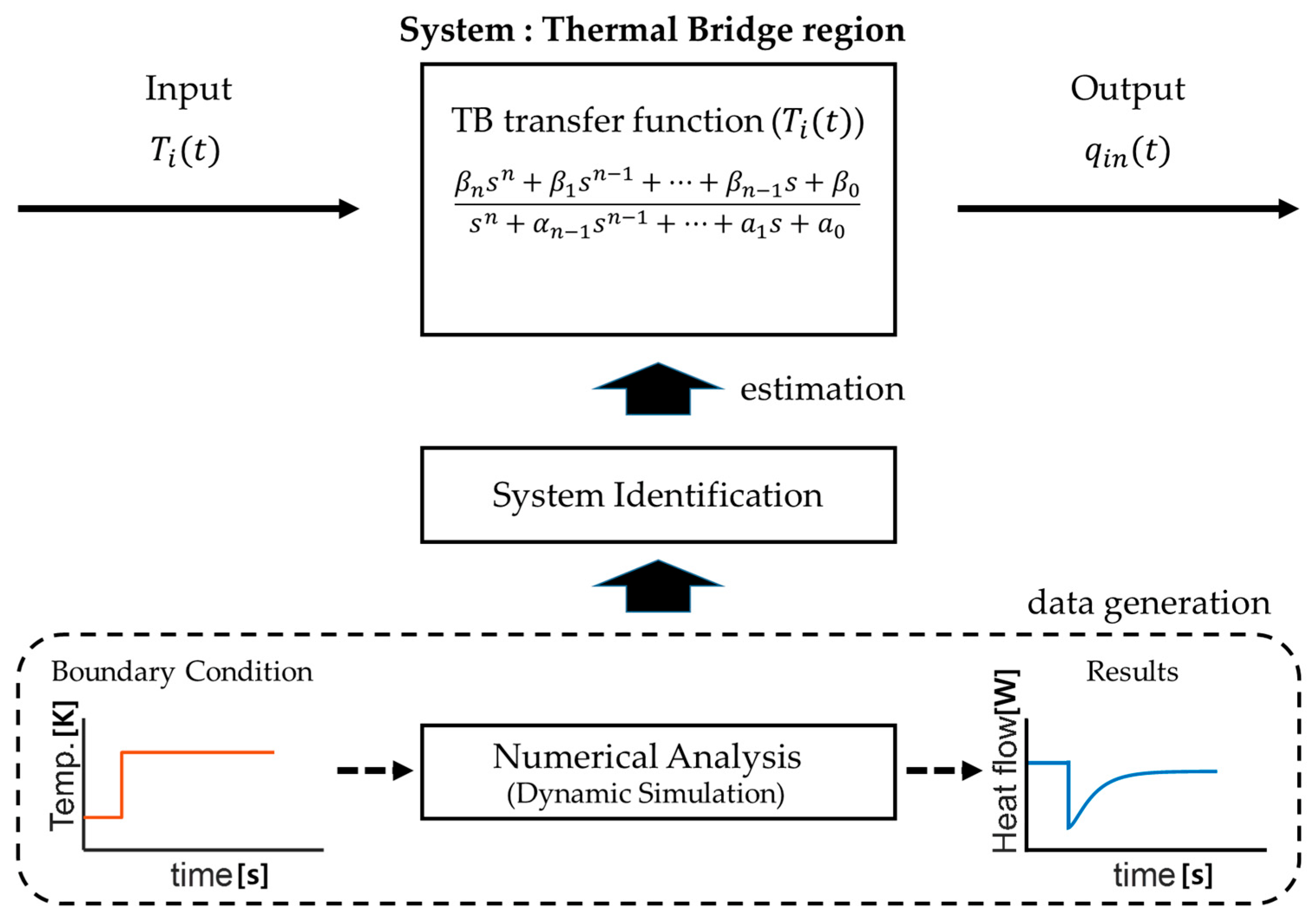
The number of poles and zeros that correspond to the system order is the same (). To distinguish this from the TB transfer function for the outdoor temperature proposed in previous studies, is added after the transfer function. The parameters that can be estimated through the system identification process are and .
To express Equation (6) more simply, it can be expressed as Equation (7) by dividing it by the parameter of the highest order of the denominator ().
Therefore, the number of parameters that can be estimated is in total, with parameters for the denominator and parameters for the numerator. The higher the system order, the more accurately the model can be estimated, but it will take slightly longer to calculate the parameters. Considering that the improvement in accuracy is not evident in the case of the 3rd-order or higher [28], in this study, the system identification is performed by increasing the order from the 1st to the 3rd order. Figure 2 shows the results of model construction and the concept of the system identification process.
3. Explanatory Example
3.1. Geometry and Materials
To validate the TB modeling method according to time-varying indoor temperature, a simple TB model is analyzed. Since the method linearly combines the transfer function for indoor temperature and the transfer function for outdoor temperature, the target building envelope with the same geometry and materials as in the previous study [28] is selected, so that the transfer function for the outdoor temperature studied in the previous study could be used. The target wall is the envelope of a typical residential building and is the same as the building envelope described in the previous research paper [28,33]. The thermal properties of the material are confirmed to be valid compared to the materials in the 2017 ASHRAE Handbook—Fundamentals. The model geometry is shown in Figure 3a, and the material dimensions and thermal properties are shown in Table 1. The first step (disaggregation stage) of the system identification process is used to determine the dimension system. To use the transfer function for the outdoor temperature studied in the previous study, the dimension system must also be the same dimension system as in the previous study; therefore, in this example, the external dimension system is determined and, accordingly, the clear wall is shown in Figure 3b.
The target wall should be able to be explained with the proposed thermal bridge model with the steady-state analysis results, as shown in Table 2. Since the geometry and material of the target wall are the same as those in the previous study, the steady-state analysis results are also the same. The steady-state analysis results are simulated using TRISCO [34], a commercial software.
3.2. System Identification and Validation Process
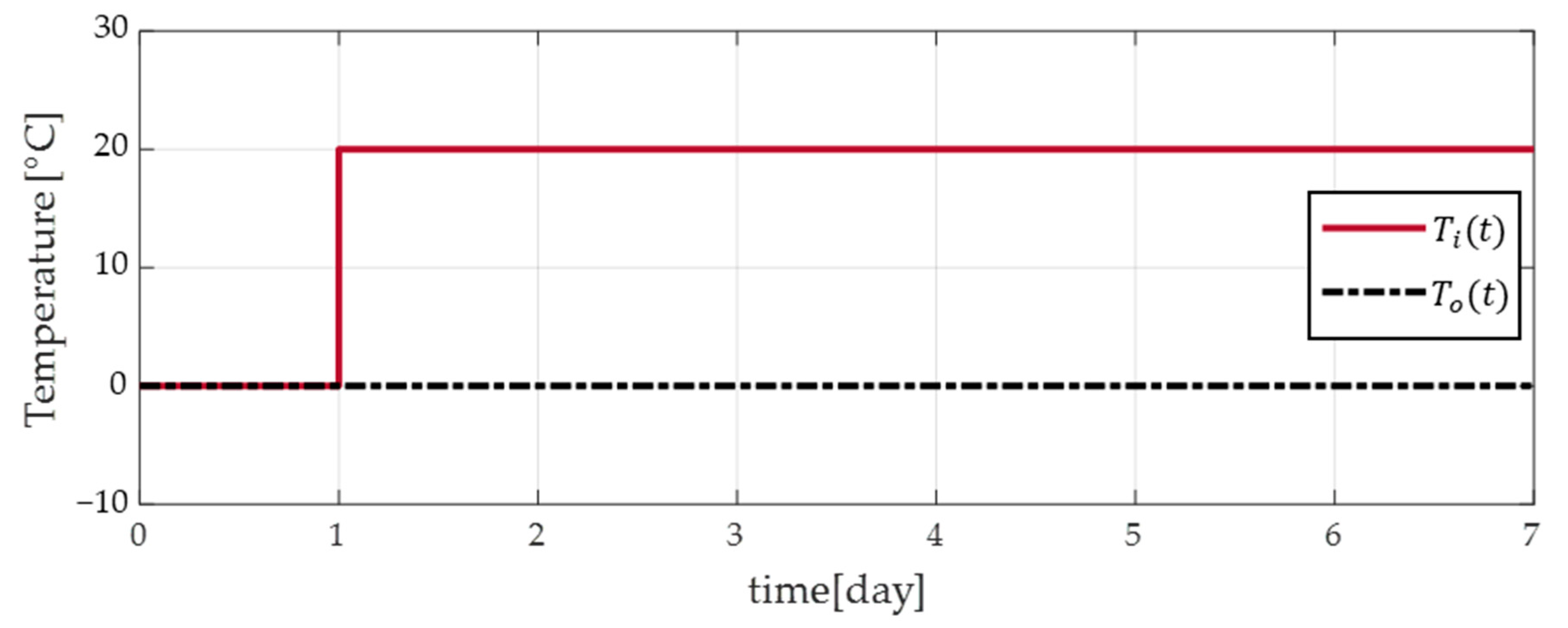
Input/output data for system identification, which correspond to step 3 of the thermal bridge modeling procedure, are needed to implement the proposed TB model. In order to obtain these data, it is necessary to perform a precise dynamic simulation of the target wall. There are many precise dynamic simulation programs for conduction phenomena with numerical analysis, such as the finite difference method (FDM), finite element method (FEM), and finite volume method (FVM) in various fields. There is little difference according to numerical analysis, and there are various methods that are mainly used in each field. In this study, VOLTRA ver. 6.0 w [35], which is widely used in the field of thermal bridge analysis, is used for obtaining the data. The input data are the time-series data of the indoor temperature and outdoor temperature that correspond to the simulation boundary condition, and the output data are the time-series data of the heat flow entering the room that corresponds to the simulation result. Since the aim of this study is to obtain the transfer function for the indoor temperature, as shown in Table 3 and Figure 4, the outdoor temperature is kept constant at 0 °C and only the indoor temperature is given as the step function from 0 °C to 20 °C after one day to obtain the data. The simulation duration is set to 20 days, which is a sufficient time to reach a steady state and the time step is set as 60 s.
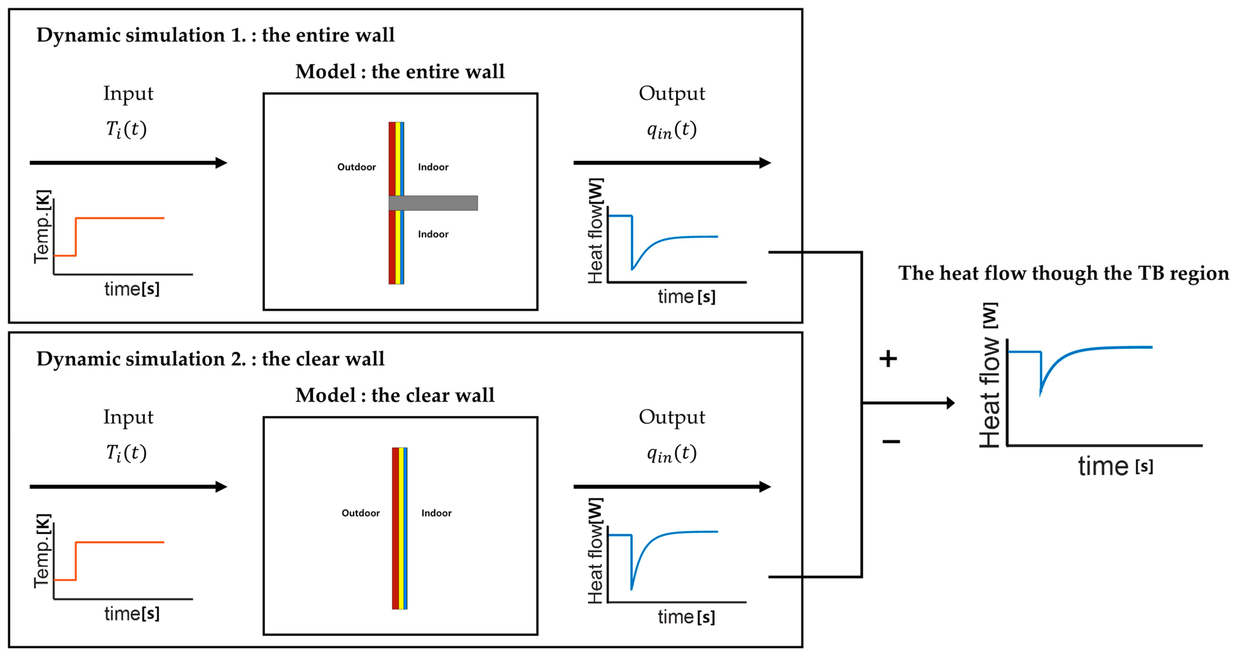
The heat flow that enters the room, which is explained using the TB model, is obtained by subtracting the heat flow that enters the room through the clear wall from the heat flow that enters the room through the entire wall. Therefore, when obtaining the time-series data of the heat flow entering the room that corresponds to the output data, the simulation result in Figure 3a and the simulation result in Figure 3b must be subtracted, so two precise dynamic simulations should be performed (Figure 5).
The parameters ( and ) are estimated using the system identification toolbox in MATLAB, using the input/output data obtained as a result of performing dynamic simulation and the form of the TB transfer function obtained through model construction (Equation (7)). Since the TB model is proposed in the form of a transfer function, Transfer Function ESTimation (“tfest”), which is a function in MATLAB, is used [36]. The higher the system order (the number of poles and the number of zeros), the higher the precision, but this is complicated and takes a significant amount of time. Therefore, in this study, system identification is performed by limiting the system order from the 1st to the 3rd order. The last step, the system identification stage, is performed to obtain the transfer function for the indoor temperature.
To validate the method proposed in this study, a two-step validation process is performed. As data-driven modeling methods can sometimes struggle to explain the given data, the first step is validation of the model itself. This step validates the step response. Since the model is estimated through the system identification process using FDM result data, the first step to check is whether the proposed model can explain the given data well. The second step is annual validation using weather data for one year, using both the proposed model (TB transfer function ()) and the transfer function for outdoor temperature, as demonstrated in previous studies. After validation is completed with the data for the creation of the model (validation of the model itself in the first step), it is necessary to validate whether it can be effectively explained using the model, even when other data are given. Since the purpose of this study is to enable the proposed TB model to be implemented in the BES, it should be validated using the outdoor temperature used in the BES, that is, weather data for one year. In this step, the indoor temperature should be a variable that changes with time, not a constant.
Figure 6 shows the outdoor and indoor temperatures for annual simulation. The outdoor temperature is the weather data in Seoul, Republic of Korea (TMY, provided by the Korean Solar Energy Society), which are used in BES, and there are 8760 annual datasets given every hour (max.: 31.3 °C; min.: −10.6 °C). The indoor temperature can be assumed to be an arbitrary value that changes with time. In this study, it is expressed as the sum of a daily sin function with an amplitude of 2 °C and an annual sin function with an amplitude of 2.5 °C, based on 22.5 °C. In addition, noise with an amplitude of 0.5 °C for each hour is randomly added to simulate an uncertain indoor temperature. This variation is assumed based on the different indoor set temperatures in summer and winter, control tolerance, sensor error, and non-uniform indoor air distribution, even if control is maintained.
The true value used for validation is the result of precise dynamic simulation. Since the dynamic simulation is the result of the numerical analysis of the governing equation using the finite difference method (FDM), this is judged to be the basis for accurately describing the physical phenomenon. Based on this FDM model, a total of five models are selected as a comparative model of the annual simulation, as shown in Table 4.
Model 1 is a steady-state model, and is a method of calculating the value obtained by multiplying the linear thermal transmittance (), which is the result of the steady-state analysis, according to the difference between the indoor and outdoor temperatures (). This is the simplest method that considers TBs in BES. Model 2 is a transfer function model for the outdoor temperature used in the previous study [28]. The TB model, assuming that the indoor temperature is constant, is selected to confirm whether this is applicable when the indoor temperature changes. Model 3 is a model in which the indoor temperature change is arithmetically corrected by using the TB model for the outdoor temperature from the previous study [28]. This approach corrects the results of the previous study by assuming that the indoor temperature changes over time, but is constant within a timestep. Models 4 to 6 linearly combine the transfer function for outdoor temperature and the transfer function for indoor temperature proposed in this study. The system order of the transfer function for the outdoor temperature is 3rd order, and the system order of the transfer function for the indoor temperature is from 1st to 3rd order. These models check the accuracy of the system order of the transfer function for the indoor temperature. Model 0 is the result of using VOLTRA, and the rest of the models are simulated using the Linear SIMulation (“lsim”) function in MATLAB [36].
4. System Identification Results and Step Response Validation
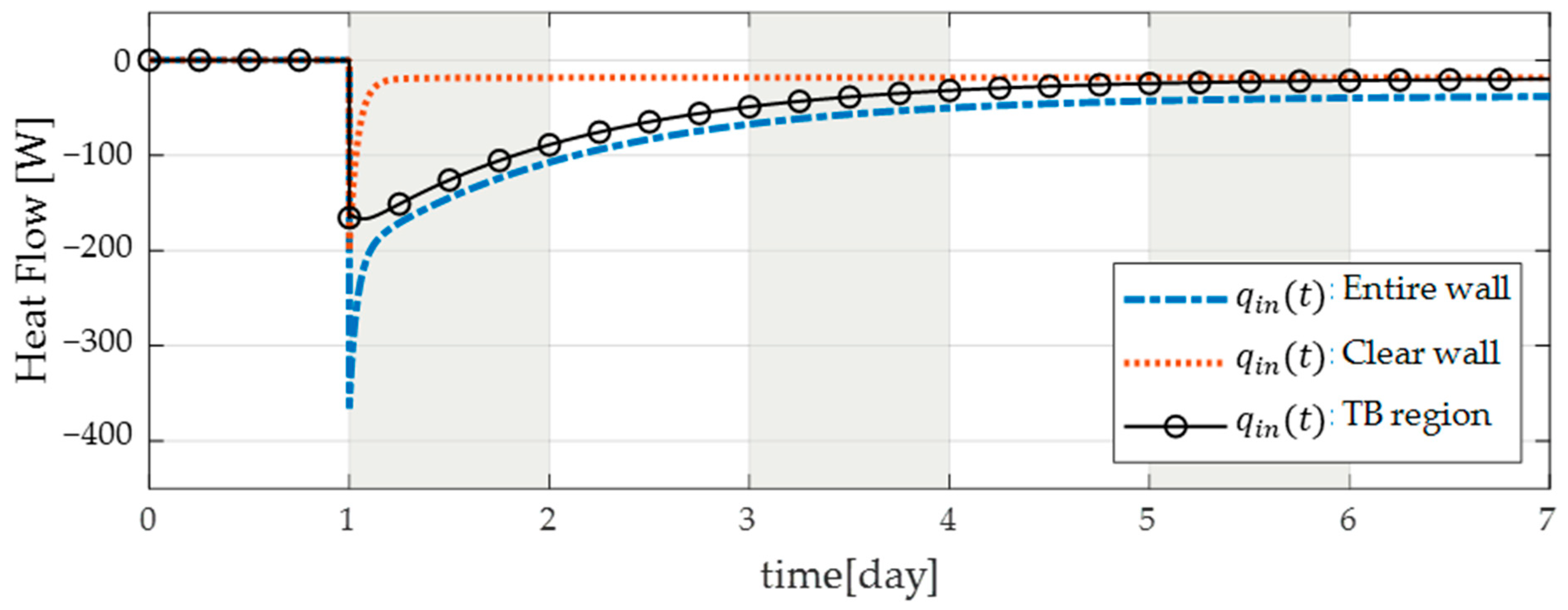
The output data for system identification (step 2 of the thermal bridge modeling procedure) are shown in Figure 7. These data are the result of performing a precise dynamic simulation of the entire wall and the clear wall, and the TB region shows the difference between the two results. Since all the indoor and outdoor temperatures are 0 °C before 1 day, and only the indoor temperature rises to 20 °C after 1 day, the heat flow that enters the room has a negative value, that is, the direction of heat flow is from the indoors to the outdoors.
Table 5 shows the results of system identification using the indoor temperature (input) in Figure 4 and the heat flow (output) that enters the room through the TB in Figure 7. In order to express the accuracy of the models, the normalized root mean square error (NRMSE), final prediction error (FPE), and mean square error (MSE) are additionally shown in Table 5. In particular, for NRMSE, the root mean square error (RMSE) is normalized with the standard deviation (), as shown in the Equation (8).
where is the measured output data, is its mean, is the simulated output data of the estimated model, and is the 2-norm. The measured output data represent the results obtained by performing the FDM simulation. A smaller NRMSE value means that the model is more accurate.
All three models show high accuracy. The NRMSE value of the model estimated by the 3rd-order system is 0.0008, which is very accurate. Estimating the model in a higher order, such as a 4th- or 5th-order system, would produce very accurate results. Although the index of the accuracy of the model is checked in Table 5, the step response results for each estimated transfer function are checked to confirm that this as a graph (Figure 8). As shown in Figure 8a, it can be confirmed that the three systems are in agreement with the FDM results to the extent that they cannot be distinguished. However, when focusing on the section where the indoor temperature suddenly changes (near one day), it can be observed that the 1st-order system changes slightly excessively (Figure 8b). The 3rd-order system is not easily distinguished from the FDM simulation results, even if it is enlarged. Taken together, system identification is properly validated from the 1st-order system to the 3rd-order system. It is confirmed that when the indoor temperature changes, a TB model in the form of a transfer function can be created that can effectively explain the heat flow that enters the room through the TB. The accuracy increases as the order of the system increases. For the TB model, the accuracy is high enough to use a 3rd-order system.
5. Annual Simulation Validation
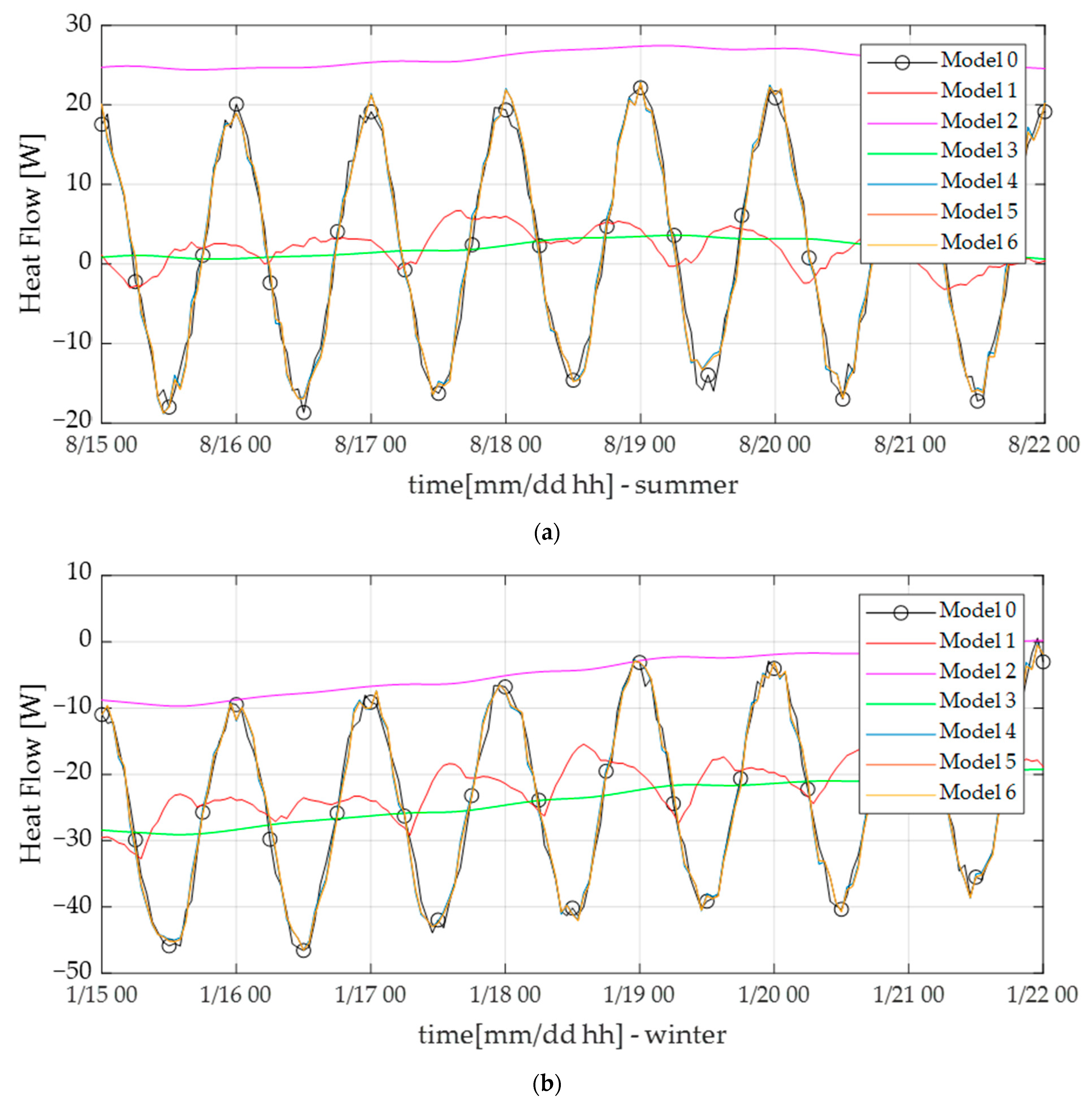
Since this study aims to create a TB model that can be implemented in BES where indoor and outdoor temperatures change over time, system identification validation alone is insufficient. Similar to performing simulations in BES, it is necessary to validate whether the proposed model is appropriate even in a situation where the outdoor temperature uses weather data and the indoor temperature changes over time in the vicinity of the set temperature. Figure 9 shows the results of the annual simulation validation, divided into summer and winter. The root meat square error (RMSE), NRMSE, and R-square were selected as the indices of accuracy, and the results are shown in Table 6. Model 0 is an FDM model, obtained by performing precise dynamic simulation, and is considered to be the true value in this study.
Model 1 is the easiest way to model the TB, as it involves multiplying the linear thermal transmittance using the indoor/outdoor temperature difference. However, the results are different from those of the FDM model. The reason for this is that, in the actual simulation, since the indoor and outdoor temperatures are dynamic and change over time, the values calculated at each time interval in the steady state do not reflect the time delay effect. The result without the time delay effect can be observed in Figure 9 as the time shift of the Model 1 and FDM model results.
Model 2 assumes that the indoor temperature is constant and only considers the change in outdoor temperature. Changes in indoor temperature are not reflected. An error occurs due to the difference between the indoor temperature (set temperature) value, which is used as a reference in TB modeling for the outdoor temperature, and the indoor temperature in the simulation. The larger this difference, the larger the error.
Model 3 is a supplementary model of Model 2, and is used to properly compensate for the indoor temperature as a constant value within one time-step. The result of this method provided the daily average value of the FDM result. However, this model seems difficult to implement in BES because of the large differences in temporal data.
Model 4 to Model 6 are all the methods proposed in this study, but the system orders of the models were as follows: 1st-, 2nd-, and 3rd-order, respectively. The results of these models are similar to the FDM results. The accuracy according to the system order is similar, and although subtle, it can be observed that the higher the order, the more accurate the model becomes. All three models have an NRMSE value of 0.1 and the R-square value of 0.99. This level of accuracy is sufficient to implement the proposed method in BES. With the addition of random noise (amplitude of 0.5 °C) to the indoor temperature in the annual simulation, the accuracy is slightly lower than that of step response validation.
6. Discussion
The thermal bridge modeling according to the time-varying indoor temperature proposed in this study is methodologically valid and the results are also verified. It was found that the system order or the number of poles and zeros of the TB transfer function affects the model accuracy, and that even the lowest order is useful to some extent. On a computer with i5-4670 CPU and 8 GB RAM, the simulation could not be performed for 1 year with a time step of 10 s and a grid size of 20 mm on the target wall, due to a lack of memory. On the other hand, it takes about 20 min to generate data using the method proposed in this study (time step: 10 s), tens of seconds to create a model using the data, and several seconds to simulate a year. It takes a significant amount of time to simultaneously perform precise dynamic simulations in BES programs, but it does not take much time when the proposed method is applied. This is because the proposed method calculates TB like a one-dimensional wall. However, it takes a significant amount of time to implement the thermal bridge model because precise dynamic simulations must be performed. Minimizing the simulation period of the precise dynamic simulation to a period that can generate enough data for system identification will help to save the overall time spent. The same issue occurs when implementing a thermal bridge model for outdoor temperature; the previous study recommended a period of about 10 days and confirmed that it should be at least 5 days [28]. In this study, as shown by Figure 7, it is necessary to perform a precise dynamic simulation for at least 5 days, because the steady state is only reached after about 5 days.
7. Conclusions
Thermal bridges that require multi-dimensional analysis are not easily analyzed in building energy simulation programs, which are one-dimensional platforms. Many studies have attempted to solve this problem, and among them, one study focuses on how to simplify the thermal bridge model and analysis on a one-dimensional platform by using data (system identification) and a similar method to that of steady-state analysis. The study proposed a method of estimating the thermal bridge model in the form of a transfer function when the indoor temperature is constant and the outdoor temperature changes. Based on the study, a method for modeling a thermal bridge is proposed and validated when both the indoor and outdoor temperatures change over time. The thermal bridge modeling method proposed in this study is essentially the same as that of the previous study.
The thermal bridge model introduced in this study is as follows.
- In the same way as in steady-state thermal bridge analysis, the thermal bridge model explains the remaining heat flow after subtracting the heat flow that enters the room through the clear wall that can be analyzed in one dimension from the heat flow that enters the room through the entire building envelope.
- The heat flow that enters the room is divided into the heat flow according to the indoor temperature and the heat flow according to the outdoor temperature, and is obtained by adding these values together.
- The thermal bridge model appears in the form of a transfer function, and is divided into the following two types: a transfer function for indoor temperature and a transfer function for outdoor temperature.
- Each thermal bridge model is estimated through system identification using data. At this time, the data are obtained using a precise dynamic analysis program and the transfer function form is determined using the number of poles and zeros by analyzing the thermal network model and considering the relationship between input (indoor temperature and outdoor temperature) and output (heat flow that enters the room) as a linear, time-invariant system.
The proposed thermal bridge model according to time-varying indoor temperature was verified using the following two steps:
- The first step: the validation of the model itself.
- -
- Validation of whether the thermal bridge model can explain the data used for system identification.
- The second step: the validation of the annual simulation.
- -
- Validation of whether the thermal bridge model can explain the random annual data.
As a result of the validation in the first step, NRMSE showed an accuracy of 0.001, and as a result of validation in the second step, NRMSE showed an accuracy of 0.1, indicating that the methodology proposed in this study is valid.
In previous studies, the third-order system of the thermal bridge transfer function for the outdoor temperature was recommended. In this study, it was also recommended that, if the system order of the thermal bridge transfer function for the indoor temperature is of the 3rd order, it is sufficiently accurate, and time can be reduced.
This method is not limited to a specific building type because it is a method of creating data for analyzing a TB and forming a ‘dynamic system’ called a thermal bridge model based on the obtained data, which can be used to simplify complex multi-dimensional analysis to one-dimensional analysis. However, since this study applied and validated only the TB geometry and material of a specific residential building based on previous studies [28,33], additional research on the validation of various geometries and materials is required. In addition, since this study focused only on the TB model that is applicable to BES, the complete building energy analysis, including the HVAC system, is not considered. Therefore, research on the implementation of the proposed TB model in BES is required. After selecting one BES program, such as EnergyPlus, to implement a TB model, it is necessary to study the BES program alone to analyze building energy, including various building elements, such as the TB, as well as the HVAC system. In terms of thermal bridge modeling, to date, it has been assumed that factors other than indoor and outdoor temperatures are constant, but in reality, they are variables that change over time. It is necessary to study how other variables that change with time, such as the convective heat transfer coefficient, should be reflected in thermal bridge modeling.
Author Contributions
Conceptualization, data curation, formal analysis, investigation, methodology, software, validation, visualization, writing—original draft preparation, writing—review and editing, H.K.; Conceptualization, data curation, formal analysis, funding acquisition, methodology, project administration, supervision, validation, writing—original draft preparation, writing—review and editing, J.K.; Conceptualization, data curation, methodology, resources, software, supervision, writing—review and editing, M.Y. All authors have read and agreed to the published version of the manuscript.
Funding
This work was supported by the National Research Foundation of Korea (NRF) grant, funded by the Korean government (MSIT) (No. 2021R1G1A1094364). In addition, the present research was supported by the research grant from Kwangwoon University in 2021 (No. 2021-0212).
Data Availability Statement
Not applicable.
Conflicts of Interest
The authors declare no conflict of interest.
Appendix A
Thermal Network Model and Transfer Function
The thermal network model is a traditional model that uses virtual heat resistance (R) and heat capacity (C) to analyze the heat transfer phenomenon through an electrical analogue [28]. This model has been applied to model the walls of buildings, whole buildings, and various components in the BES. The thermal network model can also be converted to an LTI system (via the LTI differential equation). Furthermore, the LTI system can be expressed as a transfer function. Here, the process for converting the 2R1C model into an LTI system and expressing it as a transfer function is briefly described.
- [1]
- 2R1C model
Figure A1.
The 2R1C model.
Equation (A1) describes the state of the model, and Equation (A2) describes the output of the model. When Equation (A2) is expressed with respect to , it is the same as Equation (A3).
In Equation (A1), by replacing Equation (A3) with , it is the same as Equation (A4).
Then, the LTI system for the 2R1C model can be expressed as Equation (A4). Finally, Equation (A4) is expressed as a transfer function using the Laplace transform.
Equation (A5) is the transfer function for the indoor temperature and Equation (A6) is the transfer function for the outdoor temperature.
References
- Kamel, E.; Memari, A.M. Residential Building Envelope Energy Retrofit Methods, Simulation Tools, and Example Projects: A Review of the Literature. Buildings 2022, 12, 954. [Google Scholar] [CrossRef]
- Otaegi, J.; Hernández, R.J.; Oregi, X.; Martín-Garín, A.; Rodríguez-Vidal, I. Comparative Analysis of the Effect of the Evolution of Energy Saving Regulations on the Indoor Summer Comfort of Five Homes on the Coast of the Basque Country. Buildings 2022, 12, 1047. [Google Scholar] [CrossRef]
- Emanuele, N.; Antomio, M.; Yi, Z.; Furio, B. Defining The Energy Saving Potential of Architectural Design. Energy Procedia 2015, 83, 140–146. [Google Scholar]
- Ionescu, C.; Baracu, T.; Vlad, G.E.; Necula, H.; Badea, A. The historical evolution of the energy efficient buildings. Renew. Sustain. Energy Rev. 2015, 49, 243–253. [Google Scholar] [CrossRef]
- Li, C.Z.; Zhang, L.; Liang, X.; Xiao, B.; Tam, V.W.; Lai, X.; Chen, Z. Advances in the research of building energy saving. Energy Build. 2022, 254, 111556. [Google Scholar] [CrossRef]
- Charde, M.; Gupta, R. Effect of energy efficient building elements on summer cooling of buildings. Energy Build. 2013, 67, 616–623. [Google Scholar] [CrossRef]
- Aslani, A.; Bakhtiar, A.; Akbarzadeh, M.H. Energy-efficiency technologies in the building envelope: Life cycle and adaptation assessment. J. Build. Eng. 2019, 21, 55–63. [Google Scholar] [CrossRef]
- Crawley, D.B.; Hand, J.W.; Kummert, M.; Griffith, B.T. Contrasting the capabilities of building energy performance simulation programs. Build. Environ. 2008, 43, 661–673. [Google Scholar] [CrossRef] [Green Version]
- Harish, V.; Kumar, A. A review on modeling and simulation of building energy systems. Renew. Sustain. Energy Rev. 2016, 56, 1272–1292. [Google Scholar] [CrossRef]
- Foucquier, A.; Robert, S.; Suard, F.; Stéphan, L.; Jay, A. State of the art in building modelling and energy performances prediction: A review. Renew. Sustain. Energy Rev. 2013, 23, 272–288. [Google Scholar] [CrossRef] [Green Version]
- Agdas, D.; Srinivasan, R.S. Building energy simulation and parallel computing: Opportunities and challenges. In Proceedings of the Winter Simulation Conference, Savannah, GA, USA, 7–10 December 2014; pp. 3167–3175. [Google Scholar]
- Quinten, J.; Feldheim, V. Dynamic modelling of multidimensional thermal bridges in building envelopes: Review of existing methods, application and new mixed method. Energy Build. 2016, 110, 284–293. [Google Scholar] [CrossRef]
- Ge, H.; Baba, F. Effect of dynamic modeling of thermal bridges on the energy performance of residential buildings with high thermal mass for cold climates. Sustain. Cities Soc. 2017, 34, 250–263. [Google Scholar] [CrossRef]
- Martin, K.; Erkoreka, A.; Flores, I.; Odriozola, M.; Sala, J.M. Problems in the calculation of thermal bridges in dynamic conditions. Energy Build. 2011, 43, 529–535. [Google Scholar] [CrossRef]
- Martin, K.; Campos-Celador, A.; Escudero, C.; Gómez, I.; Sala, J.M. Analysis of a thermal bridge in a guarded hot box testing facility. Energy Build. 2012, 50, 139–149. [Google Scholar] [CrossRef]
- Garay, R.; Uriarte, A.; Apraiz, I. Performance assessment of thermal bridge elements into a full scale experimental study of a building façade. Energy Build. 2014, 85, 579–591. [Google Scholar] [CrossRef] [Green Version]
- Berggren, B.; Wall, M. State of knowledge of thermal bridges—A follow up in Sweden and a review of recent research. Buildings 2018, 8, 154. [Google Scholar] [CrossRef] [Green Version]
- Zhang, X.; Jung, G.-J.; Rhee, K.-N. Performance Evaluation of Thermal Bridge Reduction Method for Balcony in Apartment Buildings. Buildings 2022, 12, 63. [Google Scholar] [CrossRef]
- Kim, M.Y.; Kim, H.G.; Kim, J.S.; Hong, G. Investigation of Thermal and Energy Performance of the Thermal Bridge Breaker for Reinforced Concrete Residential Buildings. Energies 2022, 15, 2854. [Google Scholar] [CrossRef]
- Kim, Y.H.; Kim, H.J.; Lee, H.Y. Investigation and analysis of patents for the thermal bridge breaker in green buildings. J. Korean Digit. Archit. Inter. Assoc. 2013, 13, 35–43. [Google Scholar]
- Aghasizadeh, S.; Kari, B.M.; Fayaz, R. Thermal performance of balcony thermal bridge solutions in reinforced concrete and steel frame structures. J. Build. Eng. 2022, 48, 103984. [Google Scholar] [CrossRef]
- DOE. EnergyPlus Version 22.1.0 Documentation: EnergyPlus Engineering Reference; US Department of Energy: Washington, DC, USA, 2016.
- Fiksel, A.; Thornton, J.; Klein, S.; Beckman, W. Developments to the TRNSYS simulation program. J. Sol. Energy Eng. 1995, 117, 123–127. [Google Scholar] [CrossRef]
- Kossecka, E.; Kosny, J. Equivalent wall as a dynamic model of a complex thermal structure. J. Therm. Insul. Build. Envel. 1997, 20, 249–268. [Google Scholar] [CrossRef]
- Nagata, A. A simple method to incorporate thermal bridge effects into dynamic heat load calculation programs. In Proceedings of the International IBPSA Conference, Montreal, QC, Canada, 15–18 August 2005; pp. 817–822. [Google Scholar]
- Xiaona, X.; Yi, J. Equivalent slabs approach to simulate the thermal performance of thermal bridges in building constructions. IbpsaProc. Build Simul. 2007, 10, 287–293. [Google Scholar]
- Martin, K.; Escudero, C.; Erkoreka, A.; Flores, I.; Sala, J.M. Equivalent wall method for dynamic characterisation of thermal bridges. Energy Build. 2012, 55, 704–714. [Google Scholar] [CrossRef]
- Kim, H.; Yeo, M. Thermal Bridge Modeling and a Dynamic Analysis Method Using the Analogy of a Steady-State Thermal Bridge Analysis and System Identification Process for Building Energy Simulation: Methodology and Validation. Energies 2020, 13, 4422. [Google Scholar] [CrossRef]
- Tangirala, A.K. Principles of System Identification: Theory and Practice; CRC Press: Boca Raton, FL, USA, 2018; p. 123. [Google Scholar]
- Bergman, T.L.; Incropera, F.P.; DeWitt, D.P.; Lavine, A.S. Fundamentals of Heat and Mass Transfer; John Wiley & Sons: Hobokene, NJ, USA, 2011. [Google Scholar]
- Ogata, K. System Dynamics; Pearson/Prentice Hall Englewood Cliffs: Upper Saddle River, NJ, USA, 2004; Volume 13. [Google Scholar]
- Xu, X.; Wang, S. A simplified dynamic model for existing buildings using CTF and thermal network models. Int. J. Therm. Sci. 2008, 47, 1249–1262. [Google Scholar] [CrossRef]
- Martinez, R.G.; Riverola, A.; Chemisana, D. Disaggregation process for dynamic multidimensional heat flux in building simulation. Energy Build. 2017, 148, 298–310. [Google Scholar] [CrossRef]
- PHYSIBEL. TRISCO v11.0w Manual; PHYSIBEL: Gent, Belgium, 2005. [Google Scholar]
- PHYSIBEL. VOLTRA v6.0w Manual; PHYSIBEL: Gent, Belgium, 2006. [Google Scholar]
- Matlab. MATLAB R2021b; Mathworks: Natick, MA, USA, 2021. [Google Scholar]
Figure 1.
The overall concept for building envelope analysis and thermal bridge modeling using a general approach to the modeling concept.
Figure 1.
The overall concept for building envelope analysis and thermal bridge modeling using a general approach to the modeling concept.

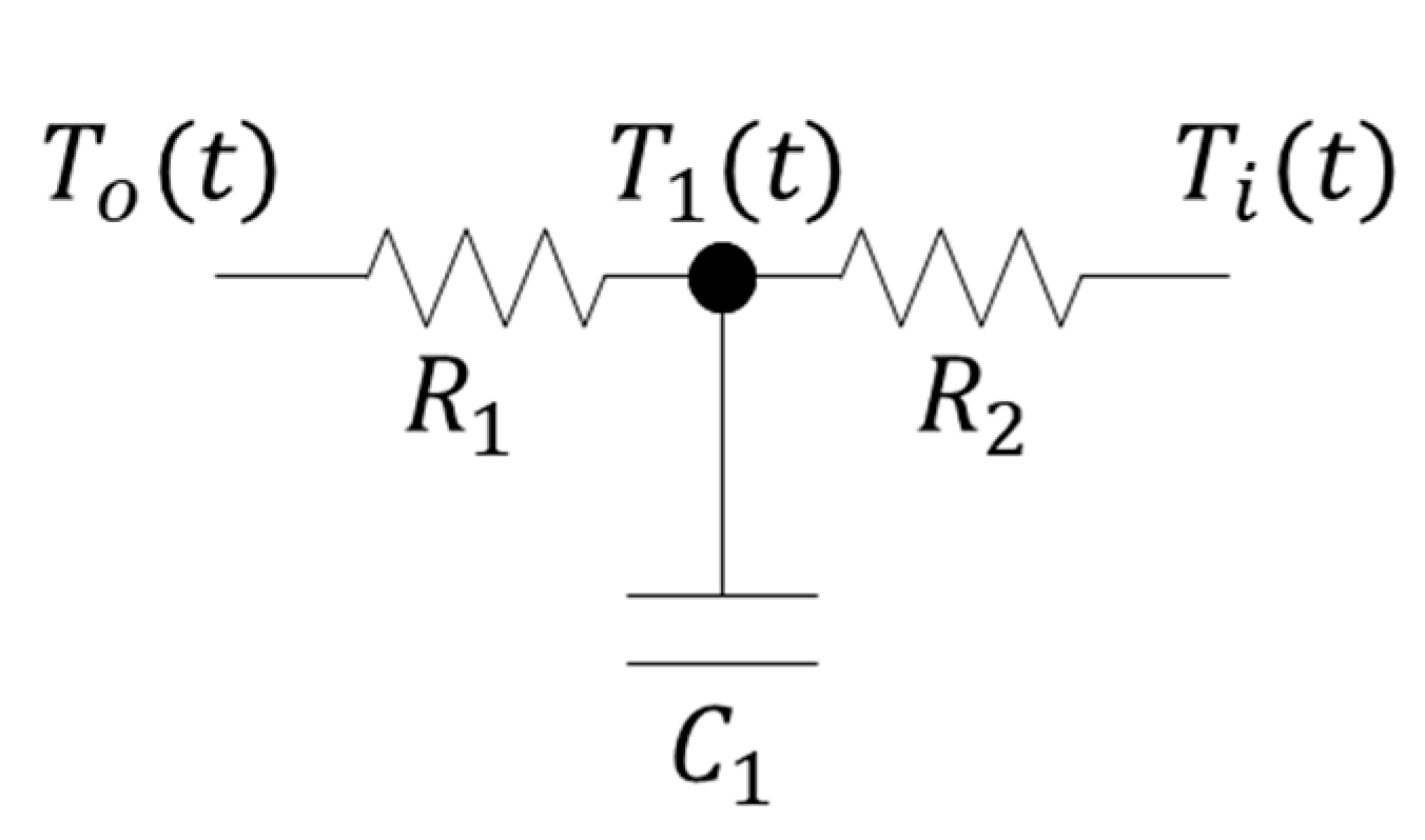
Figure 2.
The concept of the system identification process and TB transfer function form according to the indoor temperature.
Figure 2.
The concept of the system identification process and TB transfer function form according to the indoor temperature.

Figure 3.
Geometry of explanatory example: (a) the entire wall (1~9 are the material numbers in Table 1); (b) the clear wall. Red: brick, yellow: insulation (extruded polystyrene), blue: air gap, black: plasterboard, and grey: concrete “Reprinted with permission from Ref. [28]. 2020, Heegang Kim”.
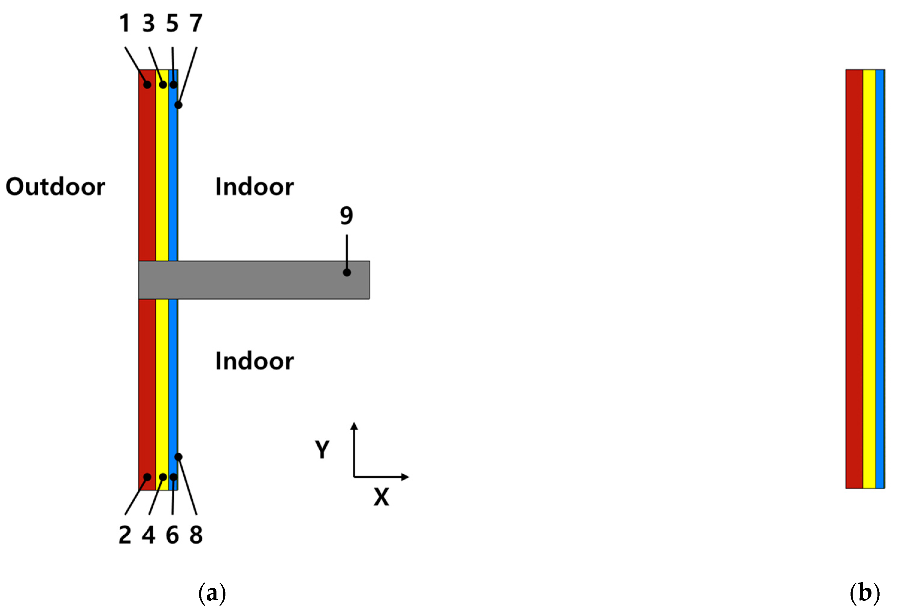
Figure 4.
Boundary conditions (the indoor temperature and the outdoor temperature) in the dynamic simulation.
Figure 4.
Boundary conditions (the indoor temperature and the outdoor temperature) in the dynamic simulation.

Figure 5.
The conceptual process for obtaining the heat flow through the TB region.

Figure 6.
Boundary conditions (the indoor temperature and the outdoor temperature) for annual simulation.
Figure 6.
Boundary conditions (the indoor temperature and the outdoor temperature) for annual simulation.
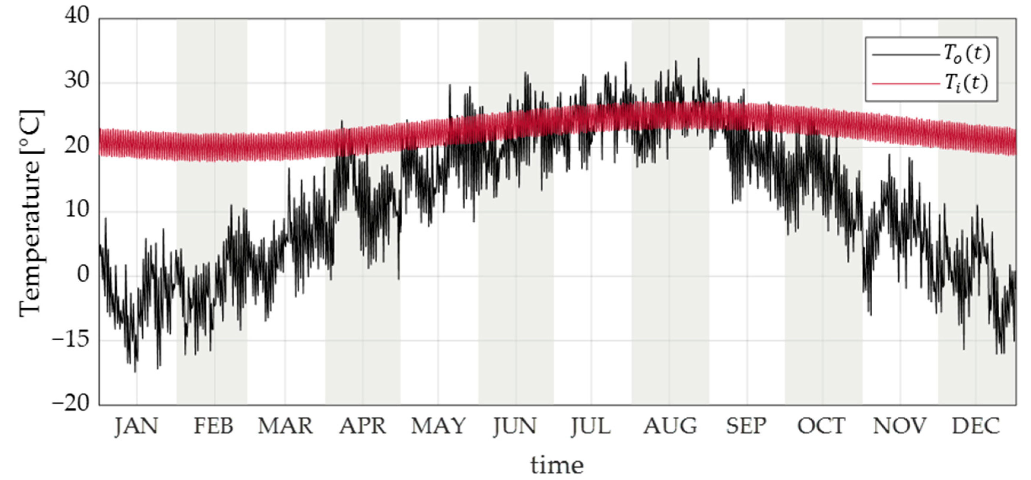
Figure 7.
The output data for system identification (dynamic simulation results).

Figure 8.
Step response of the estimated thermal bridge transfer functions for validation: (a) overall time scale; (b) zoomed time scaled around 1 day (24 h).scaled zoom at 24 h.
Figure 8.
Step response of the estimated thermal bridge transfer functions for validation: (a) overall time scale; (b) zoomed time scaled around 1 day (24 h).scaled zoom at 24 h.
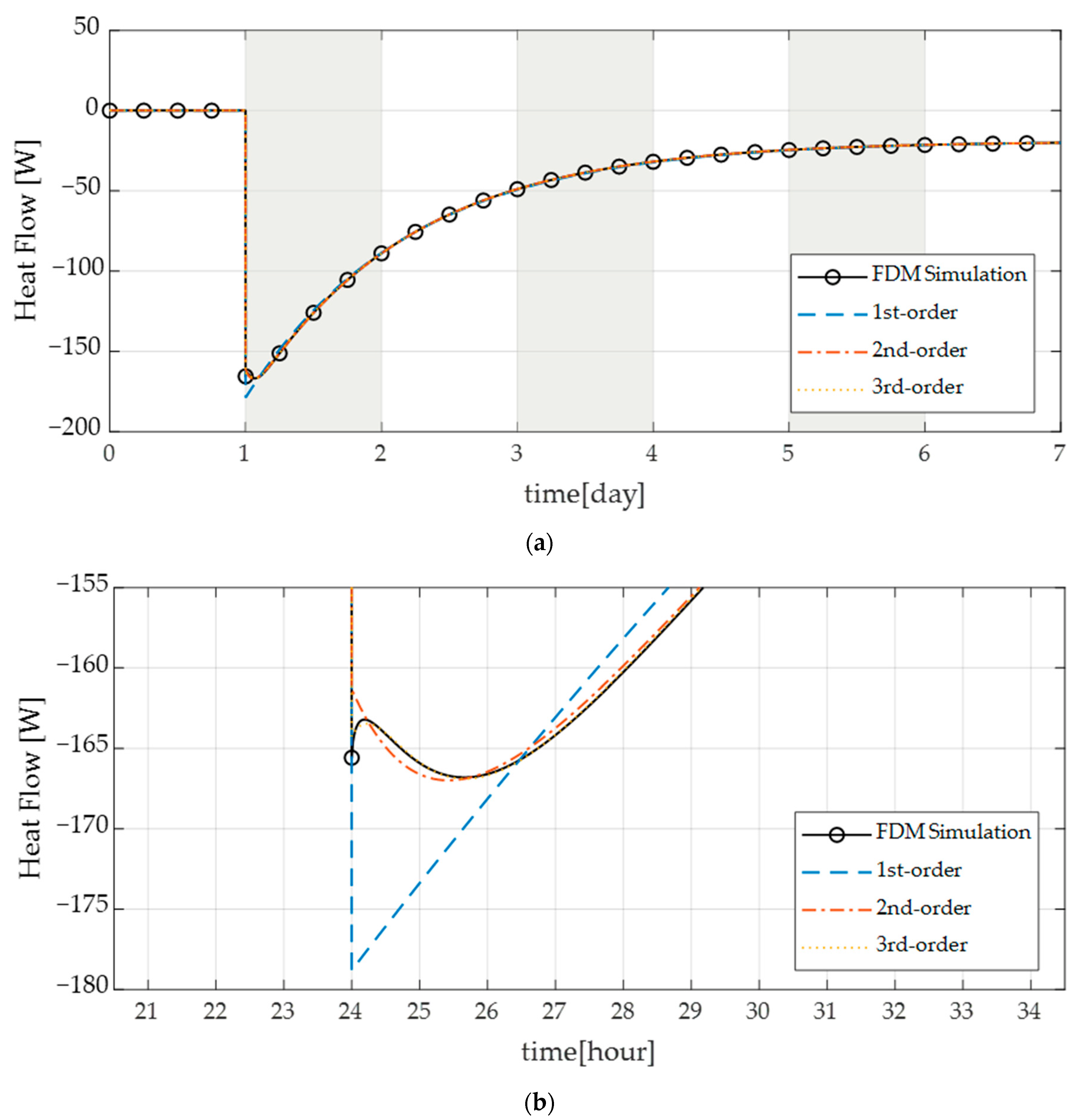
Figure 9.
Heat flow that enters the room through the TB region (annual simulation of comparative models): (a) summer; (b) winter.
Figure 9.
Heat flow that enters the room through the TB region (annual simulation of comparative models): (a) summer; (b) winter.

Table 1.
The material dimensions and thermal properties “Reprinted with permission from Ref. [28], 2020, Heegang Kim”.
Table 1.
The material dimensions and thermal properties “Reprinted with permission from Ref. [28], 2020, Heegang Kim”.
| # 1 | Material | Lx 2 (mm) | Ly 3 (mm) | 4 (W/mK) | 5 (kg/m3) | 6 (J/kgK) |
|---|---|---|---|---|---|---|
| 1 | Brick | 135 | 1500 | 0.700 | 1600.0 | 850.0 |
| 2 | 135 | 1500 | 0.700 | 1600.0 | 850.0 | |
| 3 | Extruded polystyrene | 100 | 1500 | 0.035 | 25.0 | 1470.0 |
| 4 | 100 | 1500 | 0.035 | 25.0 | 1470.0 | |
| 5 | Air gap | 65 | 1500 | 0.560 | 1.185 | 1004.4 |
| 6 | 65 | 1500 | 0.560 | 1.185 | 1004.4 | |
| 7 | Plasterboard | 10 | 1500 | 0.500 | 1300.0 | 840.0 |
| 8 | 10 | 1500 | 0.500 | 1300.0 | 840.0 | |
| 9 | Concrete | 1810 | 300 | 2.600 | 2300.0 | 930.0 |
1 #: number. 2 Lx: length (x-direction). 3 Ly: length (y-direction). 4 : thermal conductivity. 5 : density. 6 : specific heat.
Table 2.
Steady-state analysis results (grid size: 20 mm).
| Dimensional System | Thermal Transmittance | Heat Flow | ||||
|---|---|---|---|---|---|---|
| Entire Wall (W/m2K) | Clear Wall (W/m2K) | TB Region (W/mK) | Entire Wall (W) | Clear Wall (W) | TB Region (W) | |
| External | 0.6945 | 0.2980 | 1.3086 | 45.8376 | 19.6657 | 26.1719 |
Table 3.
Simulation configuration.
| Time Step | Duration | Initial Condition | Boundary Condition |
|---|---|---|---|
(20 days) | All structures and | (1 day) (1 day) |
Table 4.
Comparative models for the annual simulation.
| Model # 1 | Description |
|---|---|
| Model 0 | FDM model as exact solution |
| Model 1 | Steady-state model (T) |
| Model 2 | Only 3rd order TB transfer function |
| Model 3 | Only 3rd order TF with arithmetic correction of |
| Model 4 | 3rd order TB transfer function + 1st order TB transfer function |
| Model 5 | 3rd order TB transfer function + 2nd order TB transfer function |
| Model 6 | 3rd order TB transfer function + 3rd order TB transfer function |
1 #: number.
Table 5.
Estimated parameters for thermal bridge transfer functions (system identification results).
Table 5.
Estimated parameters for thermal bridge transfer functions (system identification results).
| System Order | First-Order | Second-Order | Third-Order | |
|---|---|---|---|---|
| Transfer Function | ||||
| # 1 of poles | 1 | 2 | 3 | |
| # 1 of zeros | 1 | 2 | 3 | |
| −9.1193 × 10⁻⁶ | −1.8796 × 10⁻⁹ | −1.7402 × 10⁻¹² | ||
| −8.9426 | −1.8304 × 10⁻³ | −1.6960 × 10⁻⁶ | ||
| - | −8.0620 | −8.0498 × 10⁻³ | ||
| - | - | −8.2158 | ||
| 9.6066 × 10⁻⁶ | 1.9727 × 10⁻⁹ | 1.8266 × 10⁻¹² | ||
| - | 2.1032 × 10⁻⁴ | 1.9551 × 10⁻⁷ | ||
| - | - | 9.9425 × 10⁻⁴ | ||
| NRMSE 2 | 0.0254 | 0.0024 | 0.0008 | |
| FPE 3 | 0.4573 | 0.0041 | 3.5690 × 10⁻⁴ | |
| MSE 4 | 0.4572 | 0.0041 | 3.5665 × 10⁻⁴ | |
1 #: number. 2 NRMSE: normalized root mean square error. 3 FPE: final prediction error for the model. 4 MSE: mean square error.
Table 6.
Accuracy of comparative model based on Model 0.
| Model 1 | Model 2 | Model 3 | Model 4 | Model 5 | Model 6 | |
|---|---|---|---|---|---|---|
| RMSE | 13.3204 | 24.9975 | 12.8481 | 1.8147 | 1.6967 | 1.6951 |
| NRMSE | 0.8772 | 1.6424 | 0.8461 | 0.1195 | 0.1117 | 0.1116 |
| R2 | 0.2396 | 0.2996 | 0.2845 | 0.9857 | 0.9875 | 0.9875 |
Publisher’s Note: MDPI stays neutral with regard to jurisdictional claims in published maps and institutional affiliations. |
© 2022 by the authors. Licensee MDPI, Basel, Switzerland. This article is an open access article distributed under the terms and conditions of the Creative Commons Attribution (CC BY) license (https://creativecommons.org/licenses/by/4.0/).
Share and Cite
MDPI and ACS Style
Kim, H.; Kim, J.; Yeo, M. Thermal Bridge Modeling According to Time-Varying Indoor Temperature for Dynamic Building Energy Simulation Using System Identification. Buildings 2022, 12, 2178. https://doi.org/10.3390/buildings12122178
AMA Style
Kim H, Kim J, Yeo M. Thermal Bridge Modeling According to Time-Varying Indoor Temperature for Dynamic Building Energy Simulation Using System Identification. Buildings. 2022; 12(12):2178. https://doi.org/10.3390/buildings12122178
Chicago/Turabian StyleKim, Heegang, Jihye Kim, and Myoungsouk Yeo. 2022. "Thermal Bridge Modeling According to Time-Varying Indoor Temperature for Dynamic Building Energy Simulation Using System Identification" Buildings 12, no. 12: 2178. https://doi.org/10.3390/buildings12122178
Note that from the first issue of 2016, this journal uses article numbers instead of page numbers. See further details here.