Wall Crack Multiclass Classification: Expertise-Based Dataset Construction and Learning Algorithms Performance Comparison

Abstract

Wall crack detection is one of the primary tasks in determining the structural integrity of a building for both restorative and preventive attempts. Machine learning techniques, such as deep learning (DL) with computer vision capabilities, have gradually become more prevalent as they can provide expert assessments with an acceptable performance when the crack detection involves a considerable number of structures. Despite such a prospective application, classification on different types of wall cracks is relatively less common, possibly due to the absence of the professional-standard-to-dataset translation. In this work, we utilised a complete pipeline, starting from novel dataset construction, ground truth formulation based on civil engineering standards, and training and testing steps. Our work focused on multi-class classification with regard to the binary classification (i.e., determining only two categories) used in previous studies. We implemented transfer learning based on VGG16 and RestNET50 for feature extraction, combined them with an ANN and kNN for the classifier, and compared their prediction performances. Our results indicate that the developed models can distinguish images that contain wall cracks into three categories of features based on the degree of damage: light, medium, and severe. Furthermore, since greyscale images offer more precise readings and predictions, the use of augmentation in dataset generation is critical. Although ResNet50 is the most stable network in terms of accuracy, it performs better when paired with kNN.

1. Introduction

The impacts of wall cracks on buildings’ reliability and aesthetics are the two most talked about points in discussions concerning building structures. Any severity level of a crack indicates an alarming situation, and can be worsened if left unchanged. As an example, a fracture in a brick wall might allow water to permeate its surface, and potentially its entire above structure. Similarly, cracked brickwork and cemented plaster can lead to various problems, such as failures in building function [1]. When the masonry becomes saturated, it can become more exposed to cold weather, causing the water to freeze and expand, and then destroying the entire structure. These examples indicate that it is imperative to make a prompt diagnosis of any cracks as early as possible to avoid further damage.

The scanned surface may show cracks and other discontinuities indicative of a poor technical condition. Fissures in walls that appear vertically or diagonally usually indicate foundation cracking. Diagonal cracks are typically found near the door and window frame corners, whereas vertical and horizontal cracks appear at the wall–column joint and in the middle of the masonry wall. Fine cracks up to 1 mm can be easily hidden by surface repair and finishing works, but larger cracks require additional measures to prevent against corrosion from the environment [2]. An examination of the crack’s orientation will help to classify the severity of the crack to determine the best method or procedure for repairing the damages [3]. Scanning for wall cracks can be one of the initial steps in the building assessment.

Analysing the amount of physical stress and its effect on materials is one of the main tasks of structural engineering assessment. In addition to studying the pattern of cracking and the rate of crack growth (or closure), a structural engineer can pinpoint the source of the problem and suggest possible solutions. This assessment process can take a long time to complete and require laborious effort as it involves various staff, especially if it applies to a bigger building. Buildings that are poorly maintained will suffer more damage and require more expensive repairs if left without attention [4]. To assess the safety and performance of the current state of concrete structures, non-destructive evaluation (NDE) techniques are commonly employed [5]. Moreover, recent studies have shown that the use of an intelligent system can aid the building assessment process [6], and can be considered as an NDE method.

Artificial intelligence (AI) has gained huge attention from many researchers in various fields. AI technology attempts to simulate and mimic human cognitive capabilities to learn and absorb information and use it to solve problems. The development of the AI area has created diverse fields, namely computer vision (CV), natural language processing (NLP), expert systems (ES), speech recognition (SR), etc.

Various methods have been developed to achieve the goal of AI to replicate human ability in a machine. The rapid development of AI created several subsets of AI that, in general, can be illustrated by Figure 1. However, in general, the main direction of AI development is to create a method that can allow machines to learn the available data. In this term, the terminology of machine learning (ML) was introduced. ML learns the data by identifying the pattern in the dataset and uses this pattern information as the basic knowledge for solving problems.

A system mixture of deep learning (DL) and computer vision can replicate various expert actions in complex building quality evaluation as envisioned in [7]. A combination of a lightweight DL model and mobile edge computing resources can serve as a remote building inspection service. A similar approach can also be applied to the inspection of passageway quality as envisaged in [8]. According to the study, a proposed model can be used to model the enclosure of a building based on the thermal property. Then, enclosures can be modelled more accurately than by using the Fourier method. As a result, the actual energy consumption of the building can be estimated more accurately [9].

Due to the importance of data, the ML performance relies on domain expertise to identify key features in the dataset. Hence, the ML technique cannot be easily implemented in different cases since it still requires human intervention for its performance. Deep learning comes later to address this problem and enhance the performance of machine learning in learning the data. Unlike conventional ML, deep learning can automatically extract the key features in the dataset and improve the pattern recognition process [10]. The key aspect of the learning process in DL methods is that it learns the data from raw representation to abstract representation with a similar procedure. Its architecture consists of multiple stacks of simple modules that map the representation of the features of the data at each level. Hence, the extraction of data representation can be simplified and automated [11]. Another work that developed a stacking-based machine learning method that is capable of detecting cracks is presented in [12]. The work assessed various most-popular object detection algorithms and then proposed a new stacking method to detect cracks near levees. As a comparison, the method performed best at 90.90%, whereas the stacking method performed comparably well at around 85%. However, the DL processes consume much more computational power than the stacking method. Therefore, without sacrificing too much accuracy, the stacking method would work better on smaller devices [12]. On the other hand, a semantic segmentation-based crack detection method exhibits a high accuracy in crack detection [13]. Despite that, fully supervised segmentation requires the manual annotation of enormous volumes of data, which is time-consuming. To address this issue, Wang (2021) presented a semi-supervised semantic segmentation network [8].

DL application on building crack detection has been proposed and evaluated in numerous works due to its ability to generalise the pattern from a dataset. The main enabler component is convolutional neural networks (CNNs), which can learn the intrinsic features of cracks from surfaces’ images. The developed capabilities make it possible to distinguish between cracks and the normal structure as reported in [14]. The study benchmarked the performance of the existing DL architecture, e.g., MobileNetV2, Restnet101, VGG16, and InceptionV2.

Similarly, the work in [15] evaluates whether a concrete segment has a crack from its visual documentation by using an artificial neural network. To perform such a task, a 10-layer CNN-based classifier was developed and trained using a dataset of 40,000 concrete crack images. The work also considered various characteristics of the concrete surface, such as the illumination and surface finish (i.e., paint, plastering, and exposed), in developing its proposed classifier. According to the study’s observation, the classifier fails to recognise cracks in images that have (1) a crack located in the corner of inputs; (2) a low resolution; (3) too small a crack.

Wall crack detection using a less complex CNN with informative reporting was proposed in [6]. The work utilised an eight-layer CNN classifier that was able to return crack segments in an image. To achieve this, the trained classifier is operated in a sliding window to detect larger resolution images. Any parts of the image that contain cracks will be assembled into a new image. A slightly different crack detection was carried out in [8], where image segments of a pavement crack were returned to user. Compared to the above-mentioned previous studies, the work applied an existing DL framework to build a classifier for an object detection purpose. The authors also investigated the effect of various sizes of the network model on the crack detection application.The image recognition method that uses the deep learning model has shown promising results in a variety of applications, including the detection of pavement cracks [16]. Several studies have pointed out the application of machine learning. Hafiz et al. showed that machine learning has surpassed the popularity of image processing for crack detection applications [17].

One of the most notable deep learning techniques that have been successfully implemented in many fields is the convolutional neural network (CNN) [18]. It has been remarkably successful in the field of computer vision. Since the beginning of its introduction, the CNN was designed to process multiple arrays in the form of an image [19].

Adha et al. used transfer learning based on CNN architecture to identify and classify buildings using the FEMA-154 classification [20]. In this work, the authors used transfer learning from the VGG16 network as the basis for developing a new model for building classification. The result from this work shows that the transfer learning technique is effective at reducing the computational effort during the model training.

Similar attempts were also performed by Pamuncak et al. by employing a transfer learning technique to reduce the computational effort on training the CNN model [21]. The authors retrained the existing CNN pre-train model to identify the bridge’s load rating. Although the bridge size only implicitly represents the bridge capacity, the trained model can still successfully extract the visual representation of the bridge capacity based on the image.

In the transfer learning process, the existence of datasets is absolutely essential and vital. Regarding crack detection on walls, researchers such as Özgenel have shared their dataset containing pre-classified images of wall cracks publicly online. Özgenel’s dataset has been used to train the deep learning algorithm [22]. Other datasets related to cracks that have also been developed include, among others: the CCIC dataset [23], the SDNET dataset [24], and the BCD dataset [25]. CCIC is collected from various buildings on the METU campus. CCIC contains 40,000 RGB images with a resolution of 227 × 227 pixels. The SDNET dataset contains more than 56,000 annotated images of cracked and non-cracked concrete bridge decks, walls, and pavements [26].

Despite the contributions made in the aforementioned works, these works mainly focus on a two-case evaluation that outputs the existence of cracks in an image input. None of these works assess the severity level of wall cracks, which can be critical in highly disaster-affected locations. In these areas, it is preferred to have a finer granularity inspection because it helps local authority to (1) survey the local buildings’ quality and (2) estimate post-disaster damage. In addition, in less-frequent disaster regions, the multi-classification system enables building tenants to self-assess and then prepare the required maintenance, avoiding potential severe damage. The following items conclude our contributions:

• We constructed a dataset of wall crack images that were collected online and then labelled according to civil engineering professional standards.
• We propose a systematic and verifiable step to construct the ground-truth data based on a combination of civil engineering standards.
• We developed eight DL models, one of which is a combined version of an existing feature extraction and classification kernel. Then, we evaluated the performance of these techniques, not only by comparing standard metrics, but also by training the convergence rate.

The remaining part of this work is organised as follows. Section 2 presents the materials and methods that were implemented in this work, including the data collection method, data pre-processing method, machine learning method for feature extraction and the classifier, and evaluation method for the trained model. Then, the results and discussion of the DL technologies used are provided in Section 3. Finally, Section 4 concludes our work.

2. Materials and Methods

2.1. Data Collection

Using a web scraper, information from websites in the form of numbers, text, images, or videos can automatically be collected. This is possible to perform by applying the web-scrapping algorithm in Python environment using Chrome driver [27]. The Chrome driver is used to control the access to web browser, and its integration with Python can automate access and save website images.

To create the dataset used in this study, several keywords were used to find related images, which are shown in

Table 1. Keywords used for the web-scrapping step.

Keywords	Number of Images Collected
#hair_crack	377 images
#wall_crack	364 images
#wall_spalling	364 images
#dinding_retak_halus*) = light wall crack	330 images
#kerusakan_plasteran_dinding*) = damage on wall plaster	350 images
#retak_dinding_non-struktural*) = non-structural wall crack	358 images
#retak_dinding_struktural*) = structural wall crack	373 images

*) keyword in Bahasa Indonesia.

. A total of 2516 images with 224 × 224 pixels with RGB channels were collected to be further processed.

2.2. Data Preprocessing

The dataset for this work was obtained by the method illustrated in Figure 2. In this work, the dataset of wall cracks was generated by the web-scraping method to extract various images in the websites based on a specific keyword that is related to the type of wall crack. However, since this scrapping technique only detects the file name and keyword of the image, many images that are not relevant to the wall crack need to be taken out from this raw data. Hence, in this phase, a screening process based on image hash and pixel similarity was conducted to remove the unsuitable and duplicate images. A total of 604 images of various types of cracks were sorted from the raw data.

The images were then manually labelled and grouped into three categories: light crack, medium crack, and severe crack. Figure 3 depicts an example of the sorting results, which illustrates the classification of cracks according to the degree of wall damage. These figures are also intended to convey the severity of the damage that occurred. The degree of crack damage on the wall was assessed using an examination of the crack pattern and visual appearance as criteria. As an outline for sorting and classification, light and moderate damage can be considered for cracks that only occur on the wall plaster. Furthermore, pictures of walls with peeling plaster and cracks in the bricks were categorised as walls with a severe degree of damage. Peeling plaster indicates that the damage to the wall has reached an alarming stage and needs to be dismantled for further investigation to be repaired.

The first author used his professional and academic experience in the field of building structure and construction to categorise the various types of cracks depicted in the collected images. In addition, to reduce bias when categorising, the first author used the current standard criteria (Table 2) as a reference. The crack size might be less convincing because the images used to make the dataset were taken from the Internet, where the shooting distances were likely to be different. On the other hand, the width of the crack was based on assumptions made by comparing the sizes of things around the crack pattern, such as door frames, windows, bricks, and others. The main focus of this article was on using machine learning to find cracks with multiclass detection using a dataset made from the images collected from the Internet, which is the limitation of this current research. For the next research stage, suggestions can be made based on improving the dataset using images with the same scale and resolution.

Due to the lack of variety in the dataset, the image augmentation technique was adopted to improve image diversity. This is important for improving the learning process and avoiding overfitting. Hence, image augmentation by rotating, flipping, and noising techniques was implemented to obtain augmented images in each class. The effect of colour in influencing the performance of the model may differ from each classification problem. One example is the use of colour information in image-based object recognition. When the recognition task is required to distinguish between instances of the same object class (intra-class classification) that normally differ in colour, the use of colour images is essential. In contrast, when the objects to be classified are from different classes that vary in shape and texture (extra-class classification), especially when objects from the same class may come in different colours, the use of colour images may be redundant. In many cases, greyscale images that preserve essential shape and texture information from their original RGB representation may be sufficient for describing classes of objects. In such cases, the use of greyscale images for classification may be more efficient [28]. However, the effect of model’s sensitiveness to colour variation to classify crack is still not fully investigated. This topic is important because using the low-quality or greyscale image will reduce the requirement for computational resources and improve the flexibility of implementing the trained model on low-resource platforms such as cellphone, Raspberry pi, etc. In summary, there were 800 images and 200 images in each class for training and validation data, respectively. Meanwhile, 50 images for each class were used as testing data. The colour transformation was then conducted to generate a greyscale dataset that contains greyscale images from the original RGB dataset.

Table 2. Crack categorisation adopted from [29,30,31].

Description	Damage Level	Numeric Literal (Class ID)
Cracks that are found in surface levels that include plaster, cement paste, mortar, and concrete. These cracks look fine and thin to human eyes, and are near but irregular in intervals. In addition, these cracks do not threaten any structural integrity and, thus, can be regarded as cosmetics cracks. Typical names that belong to this group are hairline crack, hair crack, plastic shrinkage crack, craze crack, checking, and map cracks. In addition, these cracks can possibly appear to exhibit a chequerboard pattern. Due to the minimal threat, these cracks can be easily fixed by normal decoration.	Light	0
Relatively simple cracks with a size of 1–5 mm, and up to 6 mm wide. This type of crack can be easily filled with linings to conceal its recurrent. An experienced mason can patch this crack, which requires some opening. If the cracks are less visible externally, then repointing may be needed to ensure a tight level of water.	Medium	1
This category includes cracks larger than 6 mm, and various noticeable wall damages, such as expansion and popping. Wall expansion includes swelling, softening, layer cracks, and plaster spalling. Meanwhile, popping damage encompasses fragments of conical shape that break away from the surface of the plaster, leaving behind holes of varying sizes. This crack category exhibits major wall damage, requiring partial or full reconstruction process, including sections of wall replacement.	Severe	2

Table 2. Crack categorisation adopted from [29,30,31].

Description	Damage Level	Numeric Literal (Class ID)
Cracks that are found in surface levels that include plaster, cement paste, mortar, and concrete. These cracks look fine and thin to human eyes, and are near but irregular in intervals. In addition, these cracks do not threaten any structural integrity and, thus, can be regarded as cosmetics cracks. Typical names that belong to this group are hairline crack, hair crack, plastic shrinkage crack, craze crack, checking, and map cracks. In addition, these cracks can possibly appear to exhibit a chequerboard pattern. Due to the minimal threat, these cracks can be easily fixed by normal decoration.	Light	0
Relatively simple cracks with a size of 1–5 mm, and up to 6 mm wide. This type of crack can be easily filled with linings to conceal its recurrent. An experienced mason can patch this crack, which requires some opening. If the cracks are less visible externally, then repointing may be needed to ensure a tight level of water.	Medium	1
This category includes cracks larger than 6 mm, and various noticeable wall damages, such as expansion and popping. Wall expansion includes swelling, softening, layer cracks, and plaster spalling. Meanwhile, popping damage encompasses fragments of conical shape that break away from the surface of the plaster, leaving behind holes of varying sizes. This crack category exhibits major wall damage, requiring partial or full reconstruction process, including sections of wall replacement.	Severe	2

2.3. Feature Extractor

2.3.1. VGG16 Model

Simonyan et al. (2015) proposed a ConvNet model known as VGG16 for the image classification problem that was trained by the ImageNet data set [32]. The VGG16 model accepts a 224 × 224 RGB image size as the input for the network. This model processes the input image through 18 layers constructed from convolutional and maxpooling layers to extract the most important features from the image classes. These stacks of layers are sometimes called convolution processes. The convolutional layers use a 3 × 3 kernel filter, whereas the maxpooling employs 2 × 2-pixel filters. The convolution process is followed by two fully connected layers with a size of 4096 nodes and one fully connected layer with a size of 1000 nodes. The last layer is a softmax function that transforms the result from the fully connected layer into a normalised probability distribution that can represent the probability of each output classes. Since VGG16 was trained by the ILSVRC-2012 dataset, all layer parameters in the VGG16 pre-trained model were adjusted to correctly predict the input based on ILSVRC image classes. Whilst the crack dataset is different from the ILSVRC dataset, further modifications are required to adjust the existing layer parameters in the VGG16 model to identify the wall crack classification.

In this work, the last part of the fully connected layer from the original model was then modified by reducing 1000 nodes to just 3 nodes, which represents the number of classes in our wall crack classification task. The weight of this fully connected layer was then adjusted by the re-training process using the dataset obtained from the web-scrapping technique. Accordingly, the Softmax layer output will return the probability proportion of three classes based on the forwarded output from the modified layer.

2.3.2. ResNet50 Pre-Trained Model

Deeper neural network allows for further detailed high-dimensional data interpretation for more accurate feature extraction. However, the deeper layer of the neural network will also substantially increase the complexity for model training, which may also lead to an inferior model performance. The work by He et al. [33] tried to address that problem by introducing a deep residual learning method to train the deep neural network model. The result significantly improved the training process of the deep neural model and increased the performance of the neural network model. The neural network model, named ResNet50, that was trained using the deep residual learning method won the ILSVRC 2015 and outperformed the winner from the previous year’s ILSVR competition. Since then, the ResNet50 pre-trained model has been applied to many classification tasks, and, according to a study in [34], RestNet-50 performs better in achieving a higher accuracy and lower error rate than the performances by AlexNet, GoogleNet, and VGG16 (Figure 4).

2.4. Classifier

In this work, the effectiveness of feature extraction from the pre-trained model was comparatively evaluated by two classifiers: the artificial neural network (ANN) and k-nearest neighbours (kNN). Both methods have caught the significant attention of many researchers in various fields, and there are many impressive developments in the implementation of machine learning based on both methods.

2.4.1. Artificial Neural Network (ANN)

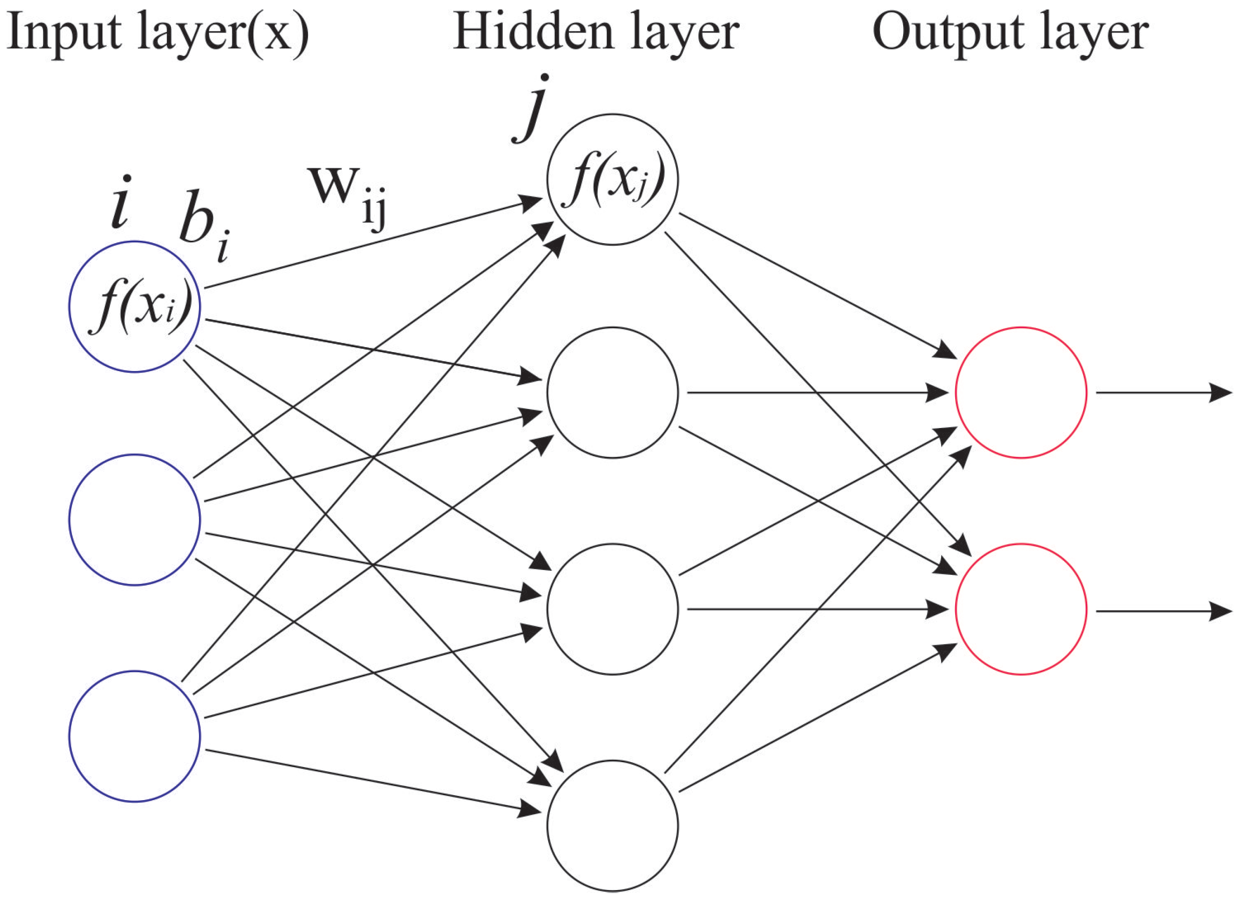
An artificial neural network is a classifier algorithm that mimics the biological process in the brain to extract any information from the external input. In general, the ANN is developed by layers of node that are divided into input, hidden, and output layers. Each node is connected to another node to receive, process, and send the impulse to the final output layers. The node is associated with its weight and activation threshold. The activation threshold is utilised as a marker to activate the node to send the signals or data to the next nodes.

In general, the artificial neural network’s layers can be illustrated by Figure 5. The process transmits signals from the receptive layers to the output layer and can be expressed as

$$x_i=f\left(\sum _j{x}_{i-1}\times w_{ij}+b_i\right),$$

where $w_{ij}$ represents the weight of the neuron connecting the nodes and $b_i$ refers to the bias value. The weight shows the important level of the input nodal contribution to the final result. Meanwhile, a bias is a constant that offsets the total product of the weight and input toward the desired result. The product of the signal process with the input, weight, and bias, which is called the activation unit, activates the nodal to transmit the signal. This activation process is determined by the threshold, which is called an activation function ($f()$). The introduction of the activation function in the neural network enables the neural network to model with a non-linear function based on the linear relation between the input, weight and bias. There are several types of activation functions introduced for the neural network, and the selection of the activation function depends on the nature of the data set. In this work, a softmax activation function was implemented, as the softmax activation function is designed for multi-class classification [36]. The softmax activation function is defined as

$$\sigma \left(z_i\right)=\frac{exp{z}_i}{{\sum }_{j}exp{z}_j}.$$

The model training process aims to optimise the neural network’s parameters, i.e., the weight and bias, so that the model can have a high performance with a high accuracy and minimum loss. Hence, the optimisation concept was implemented in the neural network to achieve that goal. The optimization process depends on the learning rate, which will direct the variable adjustment to achieve a higher model performance. After several iterations, we found that stochastic gradient descent (SGD) is more suitable for the dataset on this work as the convergence is reached faster than other optimiser methods. SGD is an extension of the gradient descent method. The general function of SGD can be mathematically written in Equation (1). However, the main difference is that, rather than checking the true gradient of the optimised function based on all data points, SGD only uses a gradient of random data points ($\nabla f_{i\left(k\right)}\left(x_k\right)$) to determine the direction of the function.

$$x_{k+1}=x_k-{\eta }_k\nabla f_{i\left(k\right)}\left(x_k\right)$$

(1)

The SGD convergence performance depends on the learning rate ratio (${\eta }_k$), which will drive the iteration to find the optimum solution. However, due to the nature of SGD, where it only employs the gradient of a random point to determine the direction of iteration, it is difficult for SGD to reach the most optimum solution, and it is sometimes stuck on endless iteration roaming around the solution or trap in local optima. Hence, determining the best learning rate is significantly important in the SGD method. There is no basic rule to determine the learning rate; however, for the problem in this work, a learning rate of 0.001 showed a good impact on the training process. Furthermore, an additional variable called momentum $\left(\beta \right)$ was also applied in this algorithm for a faster correction to reach convergence, which, in general, can be expressed by Equation (2). In this work, a momentum of 0.9 was applied on the model training process.

$$x_{k+1}=x_k-{\eta }_k(\nabla f_{i\left(k\right)}\left(x_k\right)+\beta z_{k-1})$$

(2)

2.4.2. k-Nearest Neighbor (k-NN)

Pattern recognition techniques such as k-NN have been around for a long time. This algorithm was introduced by Fix and Hodges [37]. The basic assumption of k-NN is that the things in similar classes will have similar attributes. The main process of predictions based on k-NN is to determine the closest known data to the investigated data and decide the appropriate class. The label of benchmark data should be known; thus, k-NN is also considered as a supervised machine learning algorithm. k-NN has been implemented in many fields, such as image classification [38,39,40], damage detection [41], language processing [42,43], etc.

In general, the k-NN algorithm is divided into four steps, which can be described as follows. First, the arrangement of how many neighbours (k) that will be considered to determine the class of the investigated data point. Currently, there is no qualitative research on the best k number for the general problem. However, using an odd number of neighbours is more desired in order to avoid balance counting from each classes. In this work, the classification of each data point was determined based on the class of its three neighbours. Following the procedure is the distance measurement between the selected neighbour and the investigated point according to the preferred distance formula. Here, the distance $D(x,z)$ between the investigated data point $\left(x_i\right)$ and its neighbours $\left(z_i\right)$ was calculated by using Minkowski distance Formula (3), which is described as

$$D(x,z)={\left(\sum _{i=1}^d{|x_i-z_i|}^p\right)}^{1/p}.$$

(3)

The extracted features obtained from the VGG16 and ResNet50 pre-trained model have a 1096 and 2403 dimension, respectively. Thus, the Minkowski formula was determined in the order (p) of 2 since the extracted feature from both classifiers are considered as being in high-dimensional Euclidean space. Next, the number of neighbours in each classes needs to be qualified before finally assigning the investigated data point into the class that most of the neighbours are grouped in.

2.5. Training and Validation

The training of the ANN model can take a large number of iterations/epochs. More epochs in training will increase the accuracy of the model in predicting the given training data. However, performing too many iterations in training with the same data can lead the model to overfitting the trained data. Hence, the early stopping algorithm was implemented to stop the iteration before the model overfits.

2.6. Evaluation Matrices

In this work, several evaluation matrices were used to evaluate the performance of the machine learning model. Metrics of accuracy, precision, recall, and F1 score were utilised to evaluate the model performance and to see how the model can recall the trained features and precisely utilise the feature to accurately predict the testing input. These variables can be mathematically written as follows:

$$\begin{array}{cc}\hfill \mathrm{accuracy}& =\frac{TP+TN}{TP+TN+FP+FN}\hfill \\ \hfill \mathrm{precision}& =\frac{TP}{TP+FP}\hfill \\ \hfill \mathrm{recall}& =\frac{TP}{TP+FN}\hfill \\ \hfill {\mathrm{F}1}_{score}& =2\times \frac{\mathrm{precision}\times \mathrm{recall}}{\mathrm{precision}+\mathrm{recall}}\hfill \end{array}$$

accuracy represents the proportion of correct predictions made in every class. The precision metric denotes the ratio of correct positive predictions over the total number of predicted positive labels, which represents the bias of positive predictions from the model to differentiate one class from other classes. Meanwhile, recall measures the ratio of the correctly predicted positive labels over the total real positive labels, which means the performance of the model in correctly identifying a specific class. Finally, ${\mathrm{F}1}_{score}$ is used to measure the overall performance of the model by considering the effect of precision and recall.

Furthermore, to confirm the performance of the models against the imbalance test set, the receiver operating characteristic (ROC) curve was established to illustrate the relative relationship between the true positive rate (TPR) and false positive rate (FPR) [44]. Both variables can be calculated as follows:

$$\begin{array}{cc}\hfill \mathrm{FPR}& =\frac{FP}{TN+FP},\hfill \\ \hfill \mathrm{TPR}& =\frac{TP}{TP+FN}.\hfill \end{array}$$

The true positive ($TP$), true negative ($TN$), false positive ($FP$), and false negative ($FN$) can be evaluated based on the confusion matrix described in Figure 6:

The evaluation of the model by the ROC graph was performed by transforming it into a scalar area under curve (AUC) of ROC value, which represents the expected performance. By using this scalar value, the performance of each model can be easily compared. The AUC ROV value is always between 0 and 1.

3. Result and Discussion

In this section, we present the performance metrics of the above-mentioned DL models, such as VGG16 and ResNet50, and our classifier that originates from the ANN and k-NN algorithm. There are two main observations made during the simulation: (1) the impact of a dataset’s colourspace during its training process, and (2) the impact of colour variation in the prediction.

3.1. The Effect of Colours in Model Training and Validation

Four models were investigated to evaluate their sensitivity to the colour variation. In this work, the dataset was compiled into the RGB and greyscale dataset. Before collecting the performance from the models, each model was trained by both datasets.

In terms of the learning process, the VGG16-ANN model trained with the RGB dataset reached convergence faster than the similar model trained with greyscale dataset. On training and validation datasets, the training process monitors the fluctuation in the prediction accuracy and loss of the model. The training process of the VGG16-ANN with the RGB dataset stopped on epoch 16 whereas the respective model with the greyscale dataset continued the training process until epoch 23, resulting in a higher training accuracy with lower loss. However, the investigation of Figure 7 found that the discrepancy in the accuracy caused by the variation in colour in the training dataset is not significant. The training accuracies of the last epoch of the VGG16-ANN trained with the RGB and greyscale dataset achieved 99.95% and 99.91%, respectively, whereas the loss was steady from epoch 5, with the final epoch resulting in a low loss of 1.69% for RGB and 1.49% for greyscale. A similar behaviour was shown by the VGG16-ANN model performance during its validation step. The accuracy of the last model on its validation process achieved 95.31% and 94.99% for the RGB and greyscale dataset, respectively.

On the other hand, the effect of colour variation showed a contradictory result in the ResNet50-ANN model. As depicted in Figure 8, the ResNet50-ANN model trained with the greyscale dataset can converge faster than the other model trained with RGB. The learning curve of models with th ResNet50 feature extractor increases more gradually than that of the model with the VGG16 feature extractor. However, the last epoch still resulted in the model having an accuracy of 91.05% and 88.44% for the RGB and greyscale dataset, respectively. The loss during training also gradually dropped and reached convergence, with a loss of 25.93% for RGB and 31.09% for greyscale. However, similar to the behaviour in the VGG16-ANN model, both datasets did not significantly increase the accuracy of the model. Meanwhile, in terms of the validation test, the learning process of the last epoch resulted in a validation accuracy of 93.12% and 89.06% on RGB and greyscale data, respectively, whereas the losses achieved 26.69% for RGB and 29.37% for greyscale data.

The effect of colour on the learning process of models with the kNN classifier is depicted by Figure 9. The learning performance of the kNN classifier was evaluated by investigating its cross-validation accuracy. As the pre-trained VGG16 and ResNet50 models were trained by colour images from the ImageNet dataset, the training process only affected the kNN classifier. Based on Figure 9, the learning performance of the ResNet50-kNN model is higher than the VGG16-kNN model, which means that the ResNet50 can learn faster than the VGG16 model. This behaviour is similar to the respective models with the ANN classifier. Another behaviour that can be seen from Figure 9 is that the greyscale data negatively impacted the performance of the VGG16-kNN model, whereas, in contrast, the ResNet50-kNN model was positively improved by the greyscale data. This result is in line with the training of the ANN model. Therefore, we conclude that variations in colour affect the learning process, but not in a significant manner.

The results displayed in Figure 10 show that the accuracy of all investigated models is relatively similar. However, in general, the accuracy of the model that was trained with the greyscale dataset is slightly higher than that of models trained with the RGB dataset. This finding is potentially caused by the properties of the greyscale dataset having less ambiguity in colour perception, which helps the model to better extract the feature. Furthermore, in the RGB dataset, the feature extractor should also find the feature from the crack colour, which makes the feature extraction process become more difficult compared to the feature extraction with the greyscale dataset. The greyscale model also has the advantage of having less demand for computational resources to be spent on the training process rather than RGB. This advantage is very useful for implementation in crack identification using a portable device that has a low computation capacity. Further investigation into the models’ accuracy shows that the implementation of the greyscale dataset significantly improves their accuracy, where the ResNet50-kNN models gain the highest rise by 4.5%. However, the greyscale dataset negatively affects the accuracy of the VGG16-ANN model, which reduces the accuracy by 2.44%. Thus, this result shows that implementing the ResNet50-kNN model with the greyscale dataset is a suitable combination for the crack classification task.

3.2. The Colour Variation Effect in Prediction Performance in Each Class

3.2.1. Results on RGB Model (Test 1)

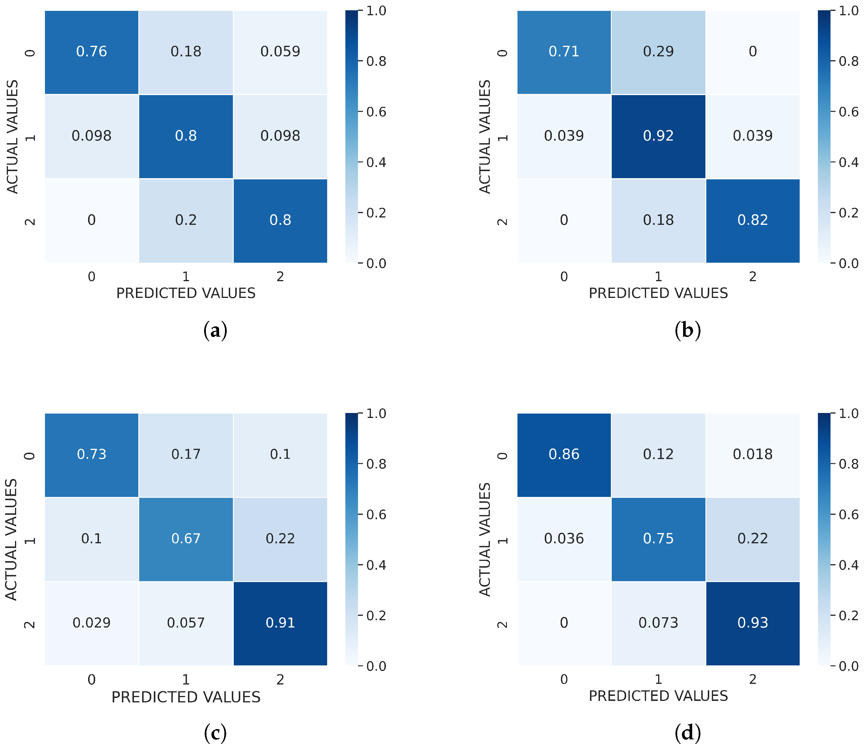
The evaluation of the model performance can be described by the confusion matrices in Figure 11.

Generally, all models can identify the input image and classify it into an appropriate class. The performance of the model in predicting each class is considerably balanced, which can be noticed by the fact that there is no high discrepancy in the correct prediction ratio in each class. The least correct prediction only appears in the ResNet50-kNN model when predicting the “Medium” class, with 66% correct predictions. Most of the highest accurate predictions appear when predicting the “Severe” class, which may be due to the noticeable features in the “Severe” class since this class is denoted by a large crack, spalling, and damaged wall. Based on the confusion matrix in Figure 11, the precision, recall, and $f{1}_{score}$ for each model are generated as shown in

Table 3. Classification performance of four models in test 1 using RGB dataset.

Description	Precision
	VGG16-ANN	ResNet50-ANN	VGG16-kNN	ResNet50-kNN
Light	0.98	0.89	0.71	0.86
Medium	0.74	0.73	0.66	0.7
Severe	0.8	0.85	0.89	0.85
Description	Recall
	VGG16-ANN	ResNet50-ANN	VGG16-kNN	Resnet50-kNN
Light	0.8	0.76	0.78	0.86
Medium	0.82	0.78	0.78	0.75
Severe	0.84	0.9	0.63	0.8
Description	F1-Score
	VGG16-ANN	Resnet50-ANN	VGG1-kNN	ResNet50-kNN
Light	0.88	0.84	0.75	0.86
Medium	0.78	0.74	0.71	0.72
Severe	0.82	0.86	0.74	0.83

.

From Table 3, the VGG16-ANN model has a greater balance performance compare to the other models based on the F1-score of 0.88. The VGG16-ANN has a higher performance in predicting “Light” and “Medium” cracks, whereas its performance for the “Severe” crack is outperformed by the ResNet50-ANN and ResNet50-kNN model.

In this work, the model performance also evaluated by using the ROC curve can be depicted as shown in Figure 12:

The ROC graph is useful for investigating the performance of the developed models in an imbalanced dataset. In this work, the imbalanced dataset was mitigated by a set of image augmentation processes to generate more augmented images in classes with fewer data. However, this augmented image may or may not significantly improve the variation in the dataset. Hence, the ROC curve was used to evaluate the performance of the model. Based on the ROC graph in Figure 12, by comparing the performance of models with the same classifier, it appears that ResNet50 performs better in extracting features than VGG16. This conclusion is drawn from the average AUCROC score of the models listed in

Table 4. Area under curve of ROC for each class based on RGB dataset.

Description	VGG16-ANN	ResNet50-ANN	VGG16-kNN	ResNet50-kNN
Light	0.97	0.98	0.87	0.92
Medium	0.91	0.91	0.84	0.85
Severe	0.93	0.96	0.83	0.9
Average AUCROC	0.94	0.95	0.85	0.89

below, which shows that the model with the ResNet50 feature extractor has a higher average AUCROC of 0.95 and 0.89 compared to the model with the VGG16 feature extractor, which only achieved a 0.95 and 0.85 score.

This result is consistent with the result illustrated in Table 3. Furthermore, it is also clearly observed that the ANN classifier has a better performance compared to the kNN classifier in the RGB dataset. By utilising the kNN classifier, a reduction in the prediction performance of the models compared to the ANN classifiers with the largest drop occurs when combining the ResNet feature extractor with the kNN classifier, resulting in a 10.75% performance drop in detecting the “severe” class. Meanwhile, the kNN classifier has less of an impact on the model than the ANN classifier. The performance drops are 6.12%, 6.59%, and 6.25% for “light”, “medium”, and “severe” classes, respectively.

3.2.2. Results on Greyscale Model (Test 2)

In this work, the effect of the greyscale image in the input was also investigated. We focused on increasing the performance of the model by reducing the complication in colour feature extraction by transforming RGB to greyscale data. The result from the model test with the greyscale dataset can be illustrated by the confusion matrix in Figure 13.

Comparing the confusion matrix from the models tested with the RGB (Figure 11) and greyscale dataset (Figure 13), the result shows that the greyscale dataset helps to improve the true positive rate of the models. However, the ResNet50-kNN model shows a significant improvement in all classes, with a 1.8%, 3.0%, and 8.0% increase in “light”, ”medium”, and “severe” classes respectively.

Considering

Table 5. Classification performance of four models in test 2 using greyscale dataset.

Description	Precision
	VGG16-ANN	Resnet50-ANN	VGG16-kNN	Resnet50-kNN
Light	0.89	0.95	0.73	0.86
Medium	0.68	0.66	0.67	0.75
Severe	0.84	0.95	0.91	0.93
Description	Recall
	VGG16-ANN	Resnet50-ANN	VGG16-kNN	ResNet50-kNN
Light	0.76	0.71	0.86	0.96
Medium	0.80	0.92	0.76	0.80
Severe	0.80	0.82	0.63	0.75
Description	F1-Score
	VGG16-ANN	ResNet50-ANN	VGG16-kNN	ResNet50-kNN
Light	0.82	0.81	0.79	0.91
Medium	0.74	0.77	0.72	0.77
Severe	0.82	0.88	0.74	0.83

, overall, ResNet50-kNN generally outperformed other models based on the F1-score. This outcome is significantly different from the previous test with the RGB dataset, where the VGG16-ANN performed better than other models. Implementing the greyscale dataset in the ResNet50-kNN model significantly increased the performance of the ResNet50-kNN model, with a significant increase of 4.35% for the “light” class and 4.71% for the “medium” class. On contrary, the combined VGG16-kNN model showed a negative impact on the model performance, with a drop of 3.57% occurring in the model performance for predicting the “Medium” class.

Based on the ROC curves shown in Figure 14, we can observe that there is no significant difference between the model performance for each class. The result indicates that the trained models are capable of distinguishing between different classes and that the unbalanced dataset has little effect on the model’s performance. Through further investigation on

Table 6. Area under curve of ROC for each class based on greyscale dataset.

Description	VGG16-ANN	ResNet50-ANN	VGG16-kNN	ResNet50-kNN
Light	0.96	0.98	0.89	0.96
Medium	0.88	0.93	0.81	0.89
Severe	0.92	0.97	0.82	0.91
Average AUCROC	0.92	0.96	0.84	0.92

, it can be concluded that the model using a greyscale dataset combined with the ResNet50 feature extractor performs better than the model using a VGG16 pretrained model as the feature extractor. By comparing Table 4 and Table 6, we found that the greyscale model with the ResNet50 feature extractor combined with the kNN classifier considerably improved by 3.26%, whereas the VGG16-ANN trained with the greyscale dataset dropped by 2.17%.

According to the work in [28], the discriminative power of features extracted from greyscale images was consistently higher than that of the RGB images when using single-layer neural network classifiers. However, the framework used in the work trained the complete network with the greyscale dataset. On the other hand, the findings in this work show that it is still possible to achieve a superior performance using a pre-trained model that is fully trained with the RGB dataset as long as that pre-trained model is coupled with a properly trained classifier with a greyscale dataset.

4. Conclusions

Crack detection on walls is carried out using convolutional neural networks as an automatic detector. In this study, we explored the general ability of the deep learning model to distinguish between three categories of wall crack features based on the degree of damage: light, medium, and severe. In the categorisation process, a collection of images from web scrapping were used as a dataset and then augmented to produce highly varied images, thus producing a more robust dataset.

The change in network usage from the VGG-ANN to ResNet50-ANN was able to provide an increase in the overall detection accuracy of 3.7% for RGB and 4.8% for the greyscale dataset. Moreover, changing the classifier type from an ANN to kNN had a more significant impact of 9.2% and 10.7% for the RGB and greyscale dataset, respectively.

Several things can be concluded from this work:

• Machine learning can be used to detect cracks in walls by utilising techniques used in image classification.
• The use of augmentation in dataset creation is essential, especially if the datasets/images are small in number.
• There is an effect of colour on the detection ability. The accuracy of the model that was trained with the greyscale dataset was slightly higher compared to the RGB dataset.
• The most promising network in providing the level of accuracy is ResNet50. Its performance can be further improved when it is combined with kNN.

References

1. Tahir, R.M. Building Component Defects Due to Land Settlement: A Case Study of Miri Industrial Training Institute. JIEI J. Ind. Eng. Innov. 2019, 1, 1–8. [Google Scholar]
2. Klimina, V.; Yurgaitis, A.; Topchiy, D. Unified classification of defects detected by the technical examination. E3S Web Conf. 2019, 110, 6–12. [Google Scholar] [CrossRef] [Green Version]
3. As’ad, S.; Mukahar; Sukiman, M. Investigation on wall crack damage and its proposed repair method. Procedia Eng. 2013, 54, 165–175. [Google Scholar] [CrossRef]
4. Suffian, A. Some common maintenance problems and building defects: Our experiences. Procedia Eng. 2013, 54, 101–108. [Google Scholar] [CrossRef] [Green Version]
5. Ohno, K.; Ohtsu, M. Crack classification in concrete based on acoustic emission. Constr. Build. Mater. 2010, 24, 2339–2346. [Google Scholar] [CrossRef]
6. Cha, Y.J.; Choi, W.; Büyüköztürk, O. Deep Learning-Based Crack Damage Detection Using Convolutional Neural Networks. Comput. Aided Civ. Infrastruct. Eng. 2017, 32, 361–378. [Google Scholar] [CrossRef]
7. Salehi, H.; Burgueño, R. Emerging artificial intelligence methods in structural engineering. Eng. Struct. 2018, 171, 170–189. [Google Scholar] [CrossRef]
8. Wang, W.; Su, C. Semi-supervised semantic segmentation network for surface crack detection. Autom. Constr. 2021, 128, 103786. [Google Scholar] [CrossRef]
9. Aznar, F.; Echarri, V.; Rizo, C.; Rizo, R. Modelling the thermal behaviour of a building facade using deep learning. PLoS ONE 2018, 13, e0207616. [Google Scholar] [CrossRef] [Green Version]
10. Majaj, N.J.; Pelli, D.G. Deep learning—Using machine learning to study biological vision. J. Vis. 2018, 18, 2. [Google Scholar] [CrossRef] [Green Version]
11. Lecun, Y.; Bengio, Y.; Hinton, G. Deep Learning. Nature 2015, 521, 436–444. [Google Scholar] [CrossRef] [PubMed]
12. Kuchi, A.; Panta, M.; Hoque, M.T.; Abdelguerfi, M.; Flanagin, M.C. A machine learning approach to detecting cracks in levees and floodwalls. Remote Sens. Appl. Soc. Environ. 2021, 22, 100513. [Google Scholar] [CrossRef]
13. Yamane, T.; Chun, P.J. Crack detection from a concrete surface image based on semantic segmentation using deep learning. J. Adv. Concr. Technol. 2020, 18, 493–504. [Google Scholar] [CrossRef]
14. Ali, S.B.; Wate, R.; Kujur, S.; Singh, A.; Kumar, S. Wall Crack Detection Using Transfer Learning-based CNN Models. In Proceedings of the 2020 IEEE 17th India Council International Conference, INDICON 2020, New Delhi, India, 10–13 December 2020. [Google Scholar] [CrossRef]
15. Le, T.T.; Nguyen, V.H.; Le, M.V. Development of deep learning model for the recognition of cracks on concrete surfaces. Appl. Comput. Intell. Soft Comput. 2021, 2021, 8858545. [Google Scholar] [CrossRef]
16. Hu, G.X.; Hu, B.L.; Yang, Z.; Huang, L.; Li, P. Pavement Crack Detection Method Based on Deep Learning Models. Wirel. Commun. Mob. Comput. 2021, 2021, 5573590. [Google Scholar] [CrossRef]
17. Munawar, H.S.; Hammad, A.W.; Haddad, A.; Soares, C.A.P.; Waller, S.T. Image-based crack detection methods: A review. Infrastructures 2021, 6, 115. [Google Scholar] [CrossRef]
18. LeCun, Y.; Boser, B.; Denker, J.; Henderson, D.; Howard, R.; Hubbard, W.; Jackel, L. Handwritten Digit Recognition with a Back-Propagation Network. In Advances in Neural Information Processing Systems; Touretzky, D., Ed.; Morgan-Kaufmann: Burlington, MA, USA, 1989; Volume 2. [Google Scholar]
19. LeCun, Y.; Bottou, L.; Bengio, Y.; Haffner, P. Gradient-based learning applied to document recognition. Proc. IEEE 1998, 86, 2278–2324. [Google Scholar] [CrossRef] [Green Version]
20. Adha, A.; Pamuncak, A.; Qiao, W.; Laory, I. Automated building classification framework using convolutional neural network. Cogent Eng. 2022, 9, 2065900. [Google Scholar] [CrossRef]
21. Pamuncak, A.; Guo, W.; Khaled, A.S.; Laory, I. Deep learning for bridge load capacity estimation in post-disaster and -conflict zones. R. Soc. Open Sci. 2019, 6, 1–7. [Google Scholar] [CrossRef] [Green Version]
22. Ko, P.; Prieto, S.A.; García de Soto, B. ABECIS: An Automated Building Exterior Crack Inspection System using UAVs, Open-Source Deep Learning and Photogrammetry. In Proceedings of the 38th International Symposium on Automation and Robotics in Construction (ISARC), Online, 2–4 November 2021; pp. 637–644. [Google Scholar] [CrossRef]
23. Özgenel, Ç.F. Concrete Crack Images for Classification, V1. Mendeley Data 2018. [Google Scholar] [CrossRef]
24. Maguire, M.; Dorafshan, S.; Thomas, R.J. SDNET2018: A Concrete Crack Image Dataset for Machine Learning Applications; Utah State University: Logan, UT, USA, 2018. [Google Scholar] [CrossRef]
25. Xu, H.; Su, X.; Wang, Y.; Cai, H.; Cui, K.; Chen, X. Automatic Bridge Crack Detection Using a Convolutional Neural Network. Appl. Sci. 2019, 9, 2867. [Google Scholar] [CrossRef] [Green Version]
26. Yang, Q.; Shi, W.; Chen, J.; Lin, W. Deep convolution neural network-based transfer learning method for civil infrastructure crack detection. Autom. Constr. 2020, 116, 103199. [Google Scholar] [CrossRef]
27. Chromium. Getting Started with ChromeDriver on Desktop. Available online: https://chromedriver.chromium.org/home (accessed on 13 September 2022).
28. Bui, H.M.; Lech, M.; Cheng, E.; Neville, K.; Burnett, I.S. Using grayscale images for object recognition with convolutional-recursive neural network. In Proceedings of the 2016 IEEE Sixth International Conference on Communications and Electronics (ICCE), Ha Long, Vietnam, 27–29 July 2016; pp. 321–325. [Google Scholar] [CrossRef]
29. Farzam, H.; Hogan, M.B.; Holub, E.P.; Kaetzel, L.J.; Luther, M.D. ACI 116R-00 Cement and Concrete Terminology Reported by ACI Committee 116 2000. pp. 1–73. Available online: http://dl.mycivil.ir/dozanani/ACI/ACI%20116R-00%20Cement%20and%20Concrete%20Terminology_MyCivil.ir.pdf (accessed on 13 September 2022).
30. Harris, C.M. Dictionary of Architecture & Construction, 4th ed.; McGraw-Hill: New York, NY, USA, 2006. [Google Scholar] [CrossRef]
31. Pool, R. Assessment of damage in low-rise buildings—Digest 251. Build. Res. Establ. 1995, 8. [Google Scholar]
32. Simonyan, K.; Zisserman, A. Very deep convolutional networks for large-scale image recognition. In Proceedings of the 3rd International Conference on Learning Representations, ICLR 2015—Conference Track Proceedings, San Diego, CA, USA, 7–9 May 2015. [Google Scholar]
33. He, K.; Zhang, X.; Ren, S.; Sun, J. Deep Residual Learning for Image Recognition. arXiv 2015, arXiv:1512.03385. [Google Scholar]
34. Ma, Y.; Zhang, P.; Tang, Y. Research on Fish Image Classification Based on Transfer Learning and Convolutional Neural Network Model. In Proceedings of the 2018 14th International Conference on Natural Computation, Fuzzy Systems and Knowledge Discovery (ICNC-FSKD), Huangshan, China, 28–30 July 2018; pp. 850–855. [Google Scholar] [CrossRef]
35. Meng, C.; Song, Y.; Ji, J.; Jia, Z.; Zhou, Z.; Gao, P.; Liu, S. Automatic classification of rural building characteristics using deep learning methods on oblique photography. Build. Simul. 2022, 15, 1161–1174. [Google Scholar] [CrossRef]
36. Bishop, C.M.; Nasrabadi, N.M. Pattern Recognition and Machine Learning, 1st ed.; Springer: Berlin/Heidelberg, Germany, 2006; Volume 4, p. 738. [Google Scholar]
37. Fix, E.; Hodges, J.L. Discriminatory Analysis. Nonparametric Discrimination: Consistency Properties. Int. Stat. Rev./Rev. Int. De Stat. 1989, 57, 238–247. [Google Scholar] [CrossRef]
38. Eyupoglu, C. Implementation of color face recognition using PCA and k-NN classifier. In Proceedings of the 2016 IEEE NW Russia Young Researchers in Electrical and Electronic Engineering Conference (EIConRusNW), St. Petersburg, Russia, 2–3 February 2016; pp. 199–202. [Google Scholar] [CrossRef]
39. Sundararaj, G.K.; Balamurugan, V. Robust classification of primary brain tumor in Computer Tomography images using K-NN and linear SVM. In Proceedings of the 2014 International Conference on Contemporary Computing and Informatics (IC3I), Mysore, India, 27–29 November 2014; pp. 1315–1319. [Google Scholar] [CrossRef]
40. Jóźwik, A.; Serpico, S.; Roli, F. A parallel network of modified 1-NN and k-NN classifiers—Application to remote-sensing image classification. Pattern Recognit. Lett. 1998, 19, 57–62. [Google Scholar] [CrossRef]
41. Feng, K.; González, A.; Casero, M. A kNN algorithm for locating and quantifying stiffness loss in a bridge from the forced vibration due to a truck crossing at low speed. Mech. Syst. Signal Process. 2021, 154, 107599. [Google Scholar] [CrossRef]
42. Kassner, N.; Schütze, H. BERT-kNN: Adding a kNN search component to pretrained language models for better QA. arXiv 2020, arXiv:2005.00766. [Google Scholar]
43. Rieger, S.A.; Muraleedharan, R.; Ramachandran, R.P. Speech based emotion recognition using spectral feature extraction and an ensemble of kNN classifiers. In Proceedings of the 9th International Symposium on Chinese Spoken Language Processing, Singapore, 12–14 September 2014; pp. 589–593. [Google Scholar] [CrossRef]
44. Fawcett, T. An introduction to ROC analysis. Pattern Recognit. Lett. 2006, 27, 861–874. [Google Scholar] [CrossRef]
Figure 1. Illustration of the interrelation of different intelligent computational techniques [7].
Buildings 12 02135 g001
Figure 2. A general overview of the project.
Buildings 12 02135 g002
Figure 3. Example of collected images from web scrapping: (a) light; (b) medium; (c) severe.
Buildings 12 02135 g003
Figure 4. ResNet structures with 50 layers (left), adapted from [35]; VGG-16 architecture (right).
Buildings 12 02135 g004
Figure 5. Schematic of artificial neural network.
Buildings 12 02135 g005
Figure 6. Confusion matrix and possible outcome of binary classification.
Buildings 12 02135 g006
Figure 7. Side-by-side comparison of the (a) training and (b) validation of VGG16-ANN models being trained on the RGB and greyscale dataset.
Buildings 12 02135 g007
Figure 8. Comparison of (a) training and (b) validation of ResNet50-ANN models trained by RGB and greyscale dataset.
Buildings 12 02135 g008
Figure 9. Comparison of cross-validation accuracy of VGG16-kNN and ResNet50-kNN models trained by RGB and greyscale dataset.
Buildings 12 02135 g009
Figure 10. Comparison of accuracy from each model in RGB and greyscale dataset.
Buildings 12 02135 g010
Figure 11. Comparison of confusion matrix for trained (a) VGG16-ANN, (b) ResNet50-ANN, (c) VGG16-kNN, and (d) ResNet50-kNN in the RGB dataset.
Buildings 12 02135 g011
Figure 12. ROC for (a) VGG16-ANN, (b) ResNet50-ANN, (c) VGG16-kNN, (d) ResNet50-kNN model in the RGB dataset.
Buildings 12 02135 g012
Figure 13. Comparison of confusion matrix for the trained (a) VGG16-ANN, (b) ResNet50-ANN, (c) VGG16-kNN, and (d) ResNet50-kNN in the greyscale dataset.
Buildings 12 02135 g013
Figure 14. ROC for (a) VGG16-ANN, (b) ResNet50-ANN, (c) VGG16-kNN, (d) ResNet50-kNN model trained with greyscale images dataset.
Buildings 12 02135 g014