Prediction of Blast-Induced Structural Response and Associated Damage Using Machine Learning

Abstract

Terrorist bombing-induced casualties are not only related to immediate fatalities but also to structural deterioration, damage, or even collapse that might occur and may lead to tremendous loss of life. Efficient assessment of blast-induced structural damage following explosion events is becoming a growing problem in modern societies. An attempt based on machine learning is made in this study to anticipate structures’ responses and the associated structural damage to reinforced concrete (RC) buildings exposed to extremely short-duration explosive loads. A program is developed to generate a set of analytically derived data for nonlinear building models subjected to explosive loads. Common machine learning models and Python libraries were utilized during the development of our program implementation to learn from a dataset. The latter has different features or input parameters, such as the amount of explosive charge, the distance from the building, fundamental period, and the building’s mass and rigidity, as well as the soil type. Our database is thus used, along with our regression-and-classification based implementations, to generate an output index that estimates and categorizes the state of damage based on the several most-important parameters of the explosion exposure. In the input database, the state of damage, based on the values of captured damage indices, is classified into one of four cases. Our code efficiently predicts those cases using a model that learns from the database. The prediction rates of the presented model reach an overall high accuracy. Therefore, the proposed model provides an accurate prediction of the level of structural damage by using the computed damage indices.

1. Introduction

Over the past several decades, the rate of terrorist attacks on civilian structures has increased all over the world. This phenomenon has become hazardous to the attacked structures and may lead to severe damage or collapse, and consequentially, social panic and loss of lives [1,2]. The challenge faced by structural designers is to design important and government structures to provide safety against numerous terroristic threats of explosion. Based on an assessment of the damage that could be caused to civil structures by terrorist attacks, quick-reconstruction strategies can be developed in which the damaged elements can be quickly restored.

Meanwhile, the dynamic response of engineering structures subjected to explosive loads has attracted more and more attention in the field of structural engineering. Several studies were conducted to appropriately investigate the intrinsic dynamic behavior of different structural components under high-intensity explosions [3]. Zhang et al. [4] studied the nature and level of damage to RC beams subjected to close-in explosive loads. Anas and Alam [5] conducted a comprehensive review of the blast response of RC slabs, and further investigation was carried out on methods of repair. Yan et al. [6] investigated the impact of explosive loads and failure characteristics on CFRP-strengthened reinforced concrete columns using numerical and experimental approaches. Additionally, a substantial number of studies were carried out to explore the effects of explosive loads on whole structures under uniform or localized blast loading [7,8].

Due to the prohibitively significant expense, explosion tests on structures cannot be easily conducted, which is especially problematic in developing countries. Furthermore, obtaining reasonably credible estimations of testing data such as explosion overpressure and structural component deformation during the explosion test is somewhat more difficult [9]. As a result, analytical or numerical approaches are commonly used to model and forecast the dynamic responses of structures under blast load. Various numerical methodologies for studying the responses of structures under blast loading in particular have been devised [10,11,12]. Nevertheless, numerical methods may still require long research plans, manpower skills, and perhaps long computation times. Nowadays, applications that are based on machine learning (ML) techniques or their older brother, artificial intelligence (AI), are literally innumerable, and they are also becoming more indispensable. Applied ML is in fact a numerical discipline, where an optimization problem is broadly nested in the core of a learning model: a search for the unknown values of the parameters that best solve or approximate the problem’s solution or fill in the numerical equation based on observed samples of data. A learning model predicts a set of terms that (hopefully) helps in calculating the relevant equation using the available data. It is not always easy to make an accurate prediction because of the nature of these data, which is typically noisy, limited, and partial, making predictions prone to inaccuracy. Nonetheless, the learning model attempts to interpret the data in order to solve the problem by creating a mapping between input and output. The accuracy of such a mapping is typically less than 100%. Like many technical fields, the booming field of ML has recently been supported by not only technological advancements but also by many researchers and developers who build on one another’s work in various pathways and disciplines. Two major drivers are the wider availability of greater data and constantly increasing computing power. The concepts of ML algorithms are not new, and neither are concerns about safety. However, predicting the effect of explosive threats on structural behavior by utilizing both numerical methods and emerging ML concepts is more contemporary and crucial. There has been a significant amount of research in the academic literature on using extensive learning techniques to identify corrosion in civil infrastructure. Convolutional neural networks (CNNs), which are one type of neural network, have particularly promising applicability for the automatic detection of image features that are less impacted by picture noise. Munawar et al. [13] suggested a modified version of extensive hierarchical CNN architecture, built on 16 convolution layers and CycleGAN, to predict pixel-wise segmentation end-to-end photos of Victoria’s Bolte Bridge and sky rail locations (Melbourne). Building damage poses a substantial threat to the structural integrity and usability of structures. Jdrzejczyk et al. [14] compared CNN and SVM algorithms for predicting multistory reinforced concrete building damage. Their research focused on a collection of residential buildings that had been subjected to mining impacts such as surface deformations and rock mass tremors throughout their technical life cycle. To create a more advanced rapid risk-based analysis methodology, Kumari et al. [15] have attempted to combine some of the most modern soft computing techniques with conventional rapid visual screening methods. The methodology offers the potential of analyzing the vulnerability of the structures in light of the aspects associated with the significance and exposure of the buildings.

Artificial neural networks (ANN), for instance, can be used to solve complicated civil engineering problems that cannot be handled by analytical methods such as analysis and design of the structures [16,17,18], damage assessment of structures [19,20], or structural control and earthquake engineering [21,22]. However, the black-box behavior of ANNs is not negligible in our case: if researchers are to think about the effects of a blast load, then they must be sure what process is going on. Afterall, the main strategic objective is to develop reconstruction strategies. Moreover, using ANNs does not provide acceptable accuracy when the dataset contains a small number of samples (unlike this research). Models that perhaps show a clearer formulation or a better efficiency than ANNs have also been considered in recent years. For instance, an evolutionary-based algorithm has been applied in [23] to evaluate the damage caused to H-section steel columns under impulsive blast loads. The results of [23] show that a classic strategy (which is based on implementing numerical investigations of a parametric finite element model using gene expression programming) offers an acceptable level of accuracy and high calculation efficiency. Additionally, in recent years, the ANN approach has been used in a number of studies, for example as shown in references [24,25,26,27,28]. A more recent ML-based model is introduced in [29] to predict the maximum displacement of reinforced concrete columns exposed to blast loading. This study is close to ours, but it uses 13 features pertaining to imperative column and blast properties based on a dataset consisting of 420 examples. Unlike [29], the study in this paper uses a larger data set to support the efficiency estimation, with a smaller number of features that are shown, both theoretically and empirically, to have a noticeable effect on classifying damage indices with the help of a simpler tree-based ML model. All this encouraged the authors of this research to further study the role that specific ML ideas would play in the dynamic response of engineering structures subjected to explosive loads based on the numerical study of their describing equations.

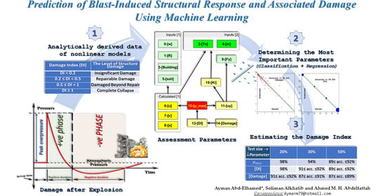
The main objective of this study is to investigate the viability of employing machine learning algorithms to anticipate the dynamic response and associated damage state of building structures subjected to bomb attacks. For this purpose, closed-form analytical solutions to the nonlinear equations of motion that govern the responses of a structure under explosive loads are first derived in order to provide a set of input data that classifies the state of damage. Consequently, a quick assessment of the damage state is conducted to identify which items are damaged and which are not, as well as to develop reconstruction procedures that provide the speedy recovery of damaged structures. The results of this study were obtained without taking the strain rate effect into consideration, and more attention should be paid in using the results in cases where strain rate effects are taken into account.

The paper is organized as follows: Section 2 presents a brief description of the blast wave pressure profile, Section 3 reports the structural damage and associated damage indices, Section 4 describes the generalized nonlinear single degree-of-freedom (SDOF) model and the closed-form solution under accidental blast loads is derived, and Section 5 connects the more theoretical part of the work to the practical part by explaining in detail how specific machine learning strategies are utilized. This longest section of the paper also presents our code implementation methodology and discusses the obtained results in detail. Finally, Section 6 summarizes the main conclusions of the work and gives suggestions for future work.

2. Blast Wave Pressure Profile

Large amounts of energy may be released after the detonation of a highly explosive chemical in an open environment. Extremely high temperatures and shock waves rapidly propagate into the surrounding air as the released energy. Shock blast waves travel at supersonic speeds and account for a significant portion of the energy produced. These waves are the most important to consider in building structural design because they reflect a building’s damage probability in an explosive event in which the front of the waves encircles the structure, exposing it to blast pressure. Figure 1 depicts the ideal blast wave pressure-time history that reaches a specific distance from the detonated charge’s center. An explosion has two distinct phases: a positive one and a negative one. During the positive phase, the pressure is higher than the ambient air pressure, and the value of the peak overpressure $P_{so}$ declines exponentially with increasing distance from the detonation center until it meets atmospheric pressure at the end of the positive phase. On the other hand, during the negative phase period (which lasts longer than the positive), the pressure falls below the ambient atmospheric pressure, generating suction on the building’s surface.

The hazard of an explosion is essentially determined by two factors, both of which are of comparable significance: (i) the explosive weight; and (ii) the stand-off distances. Hopkinson’s law converts the charge weight of the explosive $W$ in kilograms of equivalent TNT into a scaled distance $Z$ at any distance $R$ as follows (Baker et al. [30]):

$$Z=\frac{R}{W^{1/3}},$$

(1)

According to Kinny and Graham [31], the blast pressure can be described mathematically as:

$$P\left(t\right)=P_{so}\left(1-\frac{t}{t_o}\right)e^{\left(\frac{-bt}{t_o}\right)},$$

(2)

where $P_{so}$ represents the peak overpressure to represent the duration of the blast load’s positive phase, b represents the decay parameter, which is available with tabulated data varying with scaled distance $Z$ [21], and $P\left(t\right)$ represents the pressure at time $t$.

On the basis of the atmospheric pressure $P_a$ and the scaled distance $Z$, it is possible to calculate the peak overpressure $P_{so}$for an air blast in pascals as follows [31]:

$$P_{so}=\frac{808P_a\left[1+{\left(\frac{Z}{4.5}\right)}^2\right]}{{\left\{\left[1+{\left(\frac{Z}{0.048}\right)}^2\right]\left[1+{\left(\frac{Z}{0.32}\right)}^2\right]\left[1+{\left(\frac{Z}{1.35}\right)}^2\right]\right\}}^{0.5}},$$

(3)

Furthermore, the positive loading duration $t_o$ in milliseconds can take the following form [31]:

$$t_o=\frac{980W^{1/3}\left[1+{\left(\frac{Z}{0.54}\right)}^{10}\right]}{\left[1+{\left(\frac{Z}{0.02}\right)}^3\right]\left[1+{\left(\frac{Z}{0.74}\right)}^6\right]\sqrt{1+{\left(\frac{Z}{6.9}\right)}^2}},$$

(4)

3. Damage Indices

Unexpected structural responses to explosive events are of great concern nowadays. Due to the fact that the primary damage to structures is based on ductility capacity, deformation, and the global dissipated energy, these response characteristics might reflect the damage caused by destructive loads. By comparing the explosive load response characteristics to the structural capacity, a general damage index $DI$ may be calculated. Powell and Allahabadi [32] proposed a formula to define the damage index in terms of the maximum displacement $x_{max}$, the yield displacement $x_y$, and the ultimate displacement $x_u$:

$$DI=\frac{x_{max}-x_y}{x_u-x_y}=\frac{{\mu }_{max}-1}{{\mu }_u-1},$$

(5)

In Equation (5), ${\mu }_{max}$ is the maximum ductility (demand), while ${\mu }_u$ is the ultimate ductility (capacity). Buildings’ structural damage can be classified into one of the following four damage levels based on the values of the damage indices: insignificant damage, repairable damage, damaged beyond repair, and complete collapse. All the aforementioned levels of structure damage and associated damage indices are presented in

Table 1. The damage indices and associated levels of structure damage [33]. The four values in the last column are used in the implementations and results.

Damage Index ([DI])	Level of Structure Damage	[Damage] Value
DI < 0.2	insignificant damage	1
0.2 ≤ DI < 0.5	repairable damage	2
0.5 ≤ DI < 1	damaged beyond repair	3
DI ≥ 1	complete collapse	4

along with the associated values that should be used instead.

4. Modelling and Idealization

4.1. Building the Damage Model

This paper’s primary objective is to provide a two-fold way to predict the degree of damage that will be caused to building structures as a result of explosive loads. Using the measured structural responses of the mathematical models of the structures, the damage index of these structures is determined. When structures receive sudden extreme loads such as blast loads, it is inevitable that they behave extremely nonlinearly, and the dynamic response of structures goes to an inelastic range. Thereupon, nonlinear analysis is a more suitable approach capable of evaluating the realistic behavior of these structures by combining geometrical and material nonlinearities under blast loads. The simplest way to model and discretize such complex applications is via an equivalent SDOF building model that may be conveniently described by an idealized mathematical model, such as the one shown in Figure 2. The dynamic nonlinear equation of motion governing the structural response of the single-story building structure shown in Figure 2 to the blast loads shown in Figure 1 can be written as

$$m\ddot{u}\left(t\right)+c\dot{u}\left(t\right)+r\left(t\right)=f\left(t\right),$$

(6)

where $m$ and $c$ are the mass representing the inertial characteristic of the building and the viscous inherent damping coefficient representing the energy dissipation of the building, respectively; $\dot{u}\left(t\right) and \ddot{u}\left(t\right)$ denote the velocity and acceleration responses of the structure, respectively; $r\left(t\right)$ is the nonlinear restoring force, and $f\left(t\right)$ is the applied blast force to the SDOF system.

Structures always respond nonlinearly when subjected to unexpectedly extreme loads such as blast loads, and the dynamic response of the structural system goes into an inelastic region. As a result, the nonlinear analysis, which combines geometrical and material nonlinearities, provides a better approach for assessing the actual behaviors of these structures under blast loads. The SDOF building model has been regarded as elastic-perfectly plastic with elastic unloading, as illustrated in Figure 3. The relation between the SDOF system’s resistance, which is denoted by $r\left(t\right)$, and its lateral degree of freedom, which is denoted by $u$, may be divided into three different phases. During the elastic phase, resistance is expressed as $r\left(t\right)=k\times u$, whereas in the plastic phase it is expressed as $r\left(t\right)=\pm f_y$, where $k$ and $f_y$ are the structural stiffness and yield force for the structure, respectively [34]. The values of structural stiffness and damping coefficient of the SDOF building model in terms of the natural period $T_n$ and the structural damping ratio $\xi$ are determined by the following equations [35]:

$$k=\frac{4{\pi }^{2}m}{T_n^2}, c=2\xi \sqrt{k m}$$

(7)

On the other hand, the resistance force during the elastic unloading phase is given by $r\left(t\right)=u_m-k\left(u_m-u\right),$ where $u_m$ represents the structure’s maximum displacement. Depending on the magnitude and stand-off distance of the blast, the maximum displacement could be well inside the elastic range. However, if the building enters a plastic state as a result of a blast, it is presumed that the structural elements have succumbed and are damaged. Consequentially, two scenarios have been selected for analysis. In Case 1, the SDOF system’s response remains elastic during an explosion, and the maximum displacement $x_m$ occurs in an elastic condition. The blast in Case 2 occurs in an elastic state, but the maximum response occurs in a plastic state.

According to Equations (2) and (6), the explosion-loaded building model’s motion equation is

$$m\ddot{u}\left(t\right)+c\dot{u}\left(t\right)+r\left(t\right)=\left[P_{so}\left(1-\frac{t}{t_o}\right)e^{\left(\frac{-bt}{t_o}\right)}\right]A_{eq},$$

(8)

Exact solutions are obtained in the basic references for the displacement, velocity, and acceleration of the SDOF [36,37].

4.2. Formalized System Parameters

The examined building model parameters as well as the blast wave parameters used to excite the building model are defined in this section to gain further insight into the dynamic response of buildings and associated structural damage under blast loads. The dynamic characteristics of the one-story shear building models considered in the current study are listed in

Table 2. Values describing the dynamic characteristics of building models [38,39,40].

Dynamic Parameters for Building Models
Type of Parameter	Flexible [Building]	Rigid [Building]
Yielding force (N)	1.369 × 105	1.442 × 107
Damping coefficient (N-sec/m)	6.699 × 104	1.058 × 107
Range of mass (ton)	25–75	100–200
Range of natural periods (sec)	1.0–1.5	0.3–0.5

. Depending on the rigidity of the analyzed building models, the natural period of the simulated buildings ranges from roughly 0.3 to 1.5 s. Short-period vibration will occur in rigid buildings. The period of a flexible building may be larger than one second. Table 2 shows the natural period ranges for flexible and rigid buildings. Furthermore, the masses of the flexible building models ranged from 25 to 75 ton, while the rigid model mass ranged from 100 to 200 ton. Regarding the building model’s foundation, two key situations are postulated. In one of the scenarios, the supporting soil is assumed to be extremely stiff (fixed base model). In the second scenario, the effect of the soil’s flexibility is taken into account by taking into consideration the soil’s rotational and horizontal movements to account for the soil’s flexibility effect. Accordingly, there are two types of supporting soil considered in the analysis, i.e., rigid soil and flexible soil.

The story height of all models is h = 3.5 (m). It is assumed that the suggested models are fixed at their bases when analyzed during seismic occurrences, without taking into account the impact of soil-structure interaction.

In addition, the advice of several structural engineers was also adopted to determine the ranges of the explosive weights W and stand-off distances, which are presented in

Table 3. Blast load parameters used in the analysis and their ranges [2].

Parameters	Units	Ranges	Selected Values
TNT weight [w]	kg	10–2000	10, 50, 100, 500, 1000, 2000
Stand-off distance [R]	m	1.0–9.0	1, 2, 3, 5, 7, 9

. A decrease in the pressure value is represented by a wave decay coefficient (b), depending on the scaled distance Z according to W and R values listed in Table 3.

4.3. Validation

On the basis of the analytical solutions described in the preceding sections, MATLAB codes were generated for each of the analyzed cases. The proposed analytical solutions were validated by conducting a comparison of the findings acquired from the proposed methodology with those obtained in earlier studies. This served the purpose of determining whether or not the findings gained from the proposed methodology were reliable. The results were compared to those found by Li et al. [41] for the numerical system parameters in terms of mass $m$ = 100 kg, stiffness $k$ = 10000 N/m, peak explosive load $P_{so}$ = 1000 N, duration of the blast $t_o$ = 0.04 s, and maximum resistance $f_y$ = 20.042 N. As can be seen from Figure 4, the present solutions show good agreement with the solution by Li et al., and the two solutions are also clearly identical.

5. Data Treatment, Implementation Details, and Analysis

Following the presentation of the closed-form solution, an implementation pipeline for the treatment of data in cases like ours usually consists of the following steps: preparing and cleaning the data, deciding upon characteristics of the data and learning model, training the model, and evaluating the model. This section describes the cleaned data collection, gives hints on the implemented programs, shows some of the obtained results, and analyzes the results.

The dataset and its accompanying value ranges are thoughtfully chosen, which resulted in recording 1170 different cases (or table rows) of calculated observations from exciting building models in a dataset. In our investigation, two types of viscoelastic shear-type structures were modeled: fixed-base and flexible-base. A suite of reflected pressure time-histories with different TNT charge weights located at different stand-off distances ranging from 1 to 9 m are used in the analysis. The analyzed building models have fundamental periods ranging from 0.3 to 1.5 s. Our own finalized dataset consists of column labels that serve as ‘features’ of the 1170 data cases. The labels correspond to either (1) input parameters, (2) calculated parameters, or (3) output values. Elaborations on how these types and their values are put into relations can be reviewed in the equations given in the previous sections.

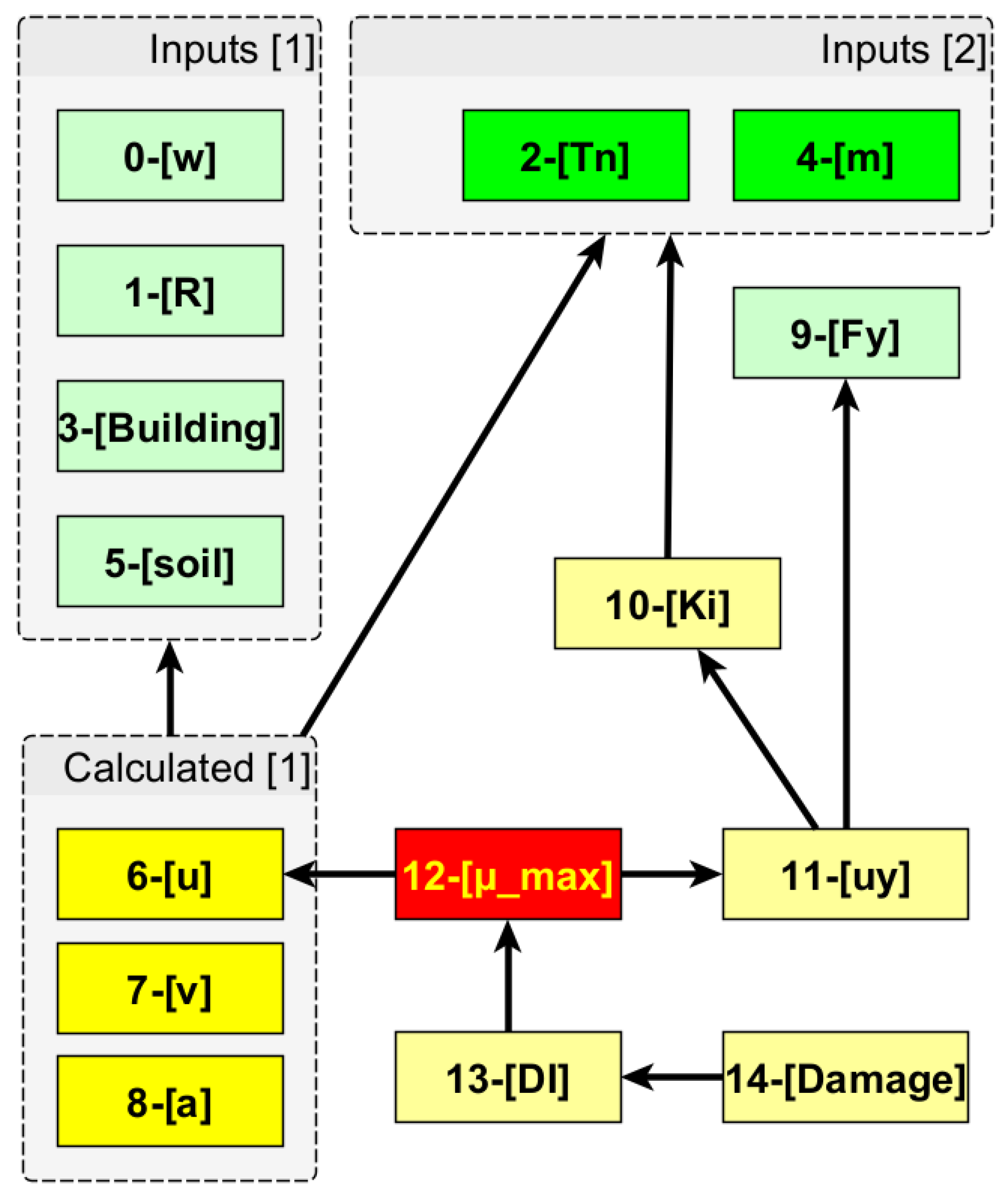
The parameters, their labels, their arrangements, and their dependency graphs are all illustrated pictorially in Figure 5 and are further verbally described in the following. Note that terms like ‘parameters’ and their ‘labels’ are commonly used in computer scientific contexts to indicate what ‘features’ would automatically be learned about the data from within the data itself. ‘Hyperparameters’ are another term used in the same contexts to indicate configurations that the program developers externally customize (manually or using heuristics; not within the data) to control or improve the learning process and its outcomes. Examples of hyperparameters are the training size and the cross-validation value (see [42] and the next subsection).

• The six ‘input parameters’ are abbreviated in the following sorted order: [w] the amount of TNT explosive charge; [R] the stand-off distance from the building; [Building] rigidity (flexible/rigid); [soil] the type of soil; [Tn] the fundamental period; and [m] the building’s mass. The subset comprising the first four labels is referred to as ‘Inputs [1]’, and the subset containing the other two input features, [Tn] and [m], as ‘Inputs [2]’ (see the top part of Figure 5).
• Except for the damage index values [DI] and the corresponding four textual labels, or [Damage] level descriptions (which are further described in the next item), the five feature parameters [u], [Fy], [Ki], [u_y], and [${\mu }_{max}$] are referred to as the ‘directly calculated parameters’. [v] and [a] are the ‘indirectly calculated’ parameters, which, together with [u], form the set of features referred to as ‘Calculated [1]’ in Figure 5.
• [DI] and [Damage] are the two ‘output’ values. [Damage]’s possible different levels are only four values, whereas [DI] values constitute a whole range of floating-point numbers. In our computer programs, [Damage] could either be treated as textual labels or four different values, depending on the need; the association is shown in Table 1.

Python was the programming language used for the development of our scripts, mainly to implement models that would efficiently learn reliable estimations of the damage levels in terms of the available input values. Both regression and classification are types of supervised learning that were implemented [43,44] depending on the cases explained below. The reader is reminded that the foundations of ML describe both regression and classification as algorithms that help predict the value of an output by finding the correlations between the dependent and the independent variables. Regression finds an approximation to a function of the input to the continuous output (e.g., a real value of the damage index [DI]), whereas classification is more of a categorization process that finds a discretizing mapping that divides the dataset into classes (e.g., when the output is one of the possible four values of the damage level [Damage]). The efficiency of the modeling is evaluated based on the resulting ‘train/test’ learning accuracy and other performance metrics of the used model, such as confusion matrix, precision, and recall [42,45]. In a regression model for example, the higher the learning accuracy, the better the estimation of further damages. Accuracy is calculated based on training the model using part of the data and testing what has been learned using the other withheld part. There is however more to this, as accuracy is a useful metric when all the classes to be learned are equally important. The situation is different in classification learning, where accuracy is not the only (or the best describing) metric. Thus, the tests performed assumed that all the classes were equally important, but the results in different situations were also studied and analyzed, particularly those where the data samples neither showed well-balanced distributions nor good representatives of the classes. For example, among the 1170 calculated samples constituting the whole dataset, only 86 belonged to the class of ‘repairable damage’, whereas as many as 208 belonged to the class of ‘total damage’. This is an important factor of analysis that should be considered in later evaluations.

5.1. Learning Damage While Considering ${\mu }_{max}$

In our computational attempts to understand how the damage index correlates to subsets of parameters using supervised machine learning [40,42], computer program feeding was tested with subsets of both ‘input’ and ‘calculated’ parameters and then determining how the learning of the output values [DI] and [Damage] was achieved.

• Learning [DI]’s (continuous) values using ‘multivariate regression’ is one way to also ‘classify’ the (discrete) level of structure [Damage] into the four categories that were taken into account, and from any given [DI] value, one immediately finds its corresponding [Damage] level (1, 2, 3, or 4) using Table 1.
• As another way, one can learn the [Damage] category using regression by assigning a value to each category, such as 1.0, 2.0, 3.0, or 4.0.
• A third way to estimate the [Damage] is to directly use a ‘classification’ algorithm (instead of regression) to learn the level of damage itself.

Different combinations of input and calculated parameters were examined to confirm the transitive dependency that is already readable from Figure 5 and our discussion in earlier sections. Keep in mind that the features should be independent in a multivariate regression. For example, it is obvious from Figure 5 that ${\mu }_{max}$ (directly) depends on both the parameters [u] and [$u_u$], which themselves depend (directly, in turn) on all the directly calculated parameters and the input parameters. The equations in Section 4 give the closed forms of such transitive dependency, but the mere values in the dataset are not enough to directly inform a supervised learning algorithm about such closed forms. The dependency, alone, does not tell us which parameters play the most- (or least-) important roles in affecting or controlling the learning result. This is exactly where the power of machine learning comes into play: the coefficients of a multivariate regression play the role of prioritizing the parameters used. This is a key goal of this research, where the data are fed into a well-designed model that uses carefully-selected parameters, then the model implementation both recognizes the indirect relationships and estimates future calculations with an evaluated accuracy. The algorithm’s ability to function through automatic learning has given us better insights into the scenario.

It is, thus, immediately noticeable from the outputs of our programs that the inclusion of μ_max among the labels to learn from is an extremely prominent situation: whenever the continuous range of [DI] values is learned using that of the calculated parameter [μ_max] (alone or in combination with other parameters) from our dataset in a regression model, an accuracy of 100% is always obtainable. This seems to be a result of overfitting, since the many values of [DI] and [μ_max] are strongly related through [DI] = 0.2 μ_max (see Section 5). The 1-1 strong link (between the many [μ_max] and [DI] values) cancels the noisy effect of the remaining parameters, whose discretized values are lower than [DI]’s or [μ_max]’s. For example, the whole dataset has only 6 different possible values for [w], [m], or [R], as well as only 2 different possible values for [soil], [Building], or [Fy]; but around 1138 different [DI] values and 1146 different [μ_max] values. Thus, and although the data have very few samples, one may even use a half of the whole dataset as training (585 representative samples) and use only four out of the six input parameters (namely: Inputs [1]), yet still obtain a nearly-perfect accuracy (again, with an obvious case of overfitting). This is true even with a ‘linear’ regression model (see Figure 6). Note that a linear regression algorithm assumes that (i) the input residuals (or errors) are normally distributed, and (ii) the input features are mutually independent (no co-linearity). According to the dependency graph in Figure 6 and the dataset experiments, both assumptions are indeed not satisfied in this case.

Although there is a nearly one-to-one correspondence between the maximum ductility ${\mu }_{max}$ values and those of [DI], there is no one-to-one correspondence between the many ${\mu }_{max}$ values and the four [Damage] values. When the [Damage] levels are represented as continuous values, the supervised learning of [Damage] (as regression) has no inherent tie in this case between the inputs to our program ([${\mu }_{max}$] in particular) and [Damage]. The obtained accuracy is still 100% as long as [${\mu }_{max}$] is among the parameters to learn from. The left chart of Figure 7 shows that the accuracy of learning is 100% using a decision tree regression model and one-fourth of the data as training samples. A linear regression model performs worse here, of course, because the relation between ${\mu }_{max}$ and [Damage] is many-to-one.

Unless explicitly specified otherwise, the ‘default assumptions’ from now on are to use a decision tree regressor or classifier (which always achieves the maximum achievable performance metrics) and 50% of the data for training, and 10-fold cross-validation.

To summarize, Equation (5) is crucial to reliably compute and learn [DI] (or, for what matters, and classify the level of structure [Damage] label). However, using available inputs, one should avoid using ${\mu }_{max}$ among the supervised learning parameters from which damage is computationally estimated. Many regression and classification algorithms will give a 100% accuracy because of overfitting. Therefore, the next ideas to learn [Damage] should take ${\mu }_{max}$ out of the equation and ask: what parameters could be important in learning the damage level?

5.2. Dropping the Role of ${\mu }_{max}$

What about directly learning [Damage] from the inputs without relying on either ${\mu }_{max}$ or [DI] values? Afterall, this is the ultimate goal: to estimate the needed output based on the available inputs. An answer is outlined in

Table 4. Highest accuracies achieved in the supervised learning of the most-important parameters that efficiently estimate the outputs: the case when all six direct inputs are used.

Test Size→ Parameter↓	20%	30%	(Default) 50%
${\mu }_{max}$	93%	90≤ acc. ≤92%	89≤ acc. ≤92%
[DI]	93%	91≤ acc. ≤92%	89≤ acc. ≤92%
[Damage]	87≤ acc. ≤90%	87≤ acc. ≤91%	87≤ acc. ≤89%

and

Table 5. Highest accuracies achieved in the supervised learning of the most-important parameters that efficiently estimate the outputs: the case when four direct inputs are used with [Ki].

Test Size→ Parameter↓	20%	30%	(Default) 50%
${\mu }_{max}$	98%	94%	89≤ acc. ≤92%
[DI]	98%	91≤ acc. ≤92%	89≤ acc. ≤92%
[Damage]	91≤ acc. ≤92%	87≤ acc. ≤91%	87≤ acc. ≤89%

and described in the following. It can be seen that the [Damage] level is learned well from specific parameters. This learning accuracy is even comparable to that of learning with ${\mu }_{max}$ or [DI].

Broadly speaking, it is more effective in reality when one anticipates the damage level based only on the purely given inputs. This avoids overfitting and unnecessary effects of the calculated parameters that are usually not readily available. This is the one side of the coin whose flip side is the closed forms and equations that were presented in earlier sections. This (i) proves that the earlier equations are applicable and (ii) increases the level of reliability of our implementations. The inherent relationships among the non-input parameters are encoded anyway in the calculated [${\mu }_{max}$], which is already in a near one-to-one relation with the [DI] values. The dataset is relatively small, which makes it sensitive to tiny changes.

Different supervised learning algorithms were applied to learn [DI] from all the parameters on which ${\mu }_{max}$ depends. An accuracy that ranged from 89% to 92% was achieved, depending on the type of algorithm used, the training-to-test ratios, and whether or not the data was normalized. A similar method was performed in order to learn [Damage] (where relatively better results were obtained).

Using only those six input parameters, it is possible to learn [DI] values as ‘features’, and we achieved a maximum accuracy of 92% using our default assumptions (i.e., using a decision tree model and 50% training). Various regressor algorithms and training/test percentages were also tested but found negligible differences. The range of obtained accuracies (for different combinations) is overall similar, with maximally ±2% difference, except in extreme cases, of course. For example, with a training set that is approximately less than 20%, the accuracy of learning [DI] values drops below 82%. With a testing set that is as low as 1%, the accuracy could reach 98%. The input combination Inputs[1] was found to always give the best accuracy, particularly when combined with [Ki], which itself encodes the two inputs of Inputs[2].

When the four [Damage] levels were learned from [${\mu }_{max}$] alone, a 99% accuracy was achieved. This is very close to the 100% achieved in the cases of the previous subsection. Unlike the previous subsection, where we included other parameters and [${\mu }_{max}$] in the learning, we learned [Damage] here only from [${\mu }_{max}$]. This further supports our earlier arguments.

With the graph dependency of Figure 5 in mind, we know that [${\mu }_{max}$] directly depends on both [u] and [$u_y$]. However, such dependency is not explicitly visible in the values of the small dataset (at least not directly visible to a machine learning-based program). Thus, when we dropped [${\mu }_{max}$] and learned [Damage] levels using only [${\mu }_{max}$]’s substitutes (namely: [u] and [$u_y$]), we did not reach 99% accuracy but rather a maximum of 96% accuracy, which could be improved to 98% with a 10% testing size, but this is not the point here. The point is that there is now some noise, and the learning model no longer has enough data samples to link [Damage] with [u] and [$u_y$] in an overfitted way.

This method of unlinking is continued by replacing one parameter with those it directly depends on (according to Figure 5) and testing the accuracy of learning the four [Damage] levels (or the [DI] values) in several ways using several combinations of parameters. In the following list, we summarize the highest accuracies obtained when some of those possible combinations were tested. Each item in the following list substitutes a parameter with those it directly depends on (see also Figure 5):

• Deciding not to overfit the learning of [DI] or [Damage] from [${\mu }_{max}$], we started learning [Damage] from [${\mu }_{max}$] alone: a 99% accuracy was achieved as described.
• Substituting [${\mu }_{max}$] with [u] and [$u_y$] in the previous combination: the maximum accuracy achieved in learning [Damage] was 96% under our ‘default assumptions’. Learning the many [DI] values from the same labels achieved a maximum accuracy of 92%. This means (according to our dataset) that it is better to learn [Damage] levels directly from [u] and [$u_y$] using a decision tree regressor and a test size of 50% than to learn the nearly one thousand [DI] values (and then use Table 1 to find corresponding [Damage] levels).
• Substituting in the previous combination for [$u_y$] (i.e., learning [Damage] from [u], [Fy], and [Ki]): the maximum accuracy achieved was still 96%. Learning [DI] values from the same labels achieved a maximum accuracy of 90%. Again, it seems better to learn [Damage] than to learn [DI] (using the current adjustments and the examined combination of labels).
• Substituting [Ki] with [Tn] and [m] in the previous combination: the maximum accuracy achieved for learning [Damage] from the labels [u], [Fy], [m], and [Tn] was 95%. Learning [DI] values from the same labels achieved a maximum accuracy of 89%
• Substituting [u] with the remaining four inputs in the previous combination: the maximum accuracy achieved for learning [Damage] from the labels [w], [R], [Building], [soil], [Fy], [m], and [Tn] was substantially lowered (from 95% in the previous case) to 89%. Learning [DI] values from the same labels, on the other hand, increased to a maximum accuracy of 92%.
• Maximum accuracy of 89% was maintained even after further reducing [Fy] and learning [Damage] in terms of only the six direct input parameters.

The existence of [Fy] does not very much affect the accuracy in any of the studied cases. Remember that [Fy] has exactly two possible different values. One would conjecture that the ‘decision’ about the damage level is not very much affected by yield force as much as it is affected by structural stiffness [Ki] in cases of explosion. For this, we tested the cases where we used neither of the two inputs on which both [Ki] and [u] depend (namely: [Tn] and [m]), but rather only learned from: (i) Inputs [1], (ii) [Ki], and (iii) [Fy]. The results were found to be exactly the same whether or not [Fy] was included. In other words, (1) [Damage] is learned with a maximum accuracy of ≤ 90%; and (2) [DI] is learned with a maximum accuracy of ≤ 93%. Furthermore, the five labels to learn from (namely Inputs [1] and [Ki]) yield better accuracies than those obtained while using all of six inputs or while using only ‘Inputs [1]’.

To sum up, based on the results in this subsection, it is both normal and advisable to use only input parameters to estimate a [Damage] level. However, the accuracy of estimation is empirically at its best when only the five combinations of parameters Inputs [1] and [Ki] are all included in the learning, while at the same time dropping the parameters [Fy], [Tn], and [m] (see Table 4 and Table 5). Table 4 lists the highest accuracies achieved when learning ${\mu }_{max}$, [DI] values, and [Damage] levels when all six input parameters were directly used. As shown in Table 5, the outcomes were similar when learning was based solely on the combination of Inputs [1] and [Ki]. It is clear from comparing the results in the two tables that the latter approach gives better results.

6. Conclusions

The findings of this study shed light on various aspects of the significant problem of blast-induced structural damage that occurs following explosive events. The aspects are investigated in a dual way, coupling ideas from numerical techniques and artificial intelligence. Equations governing the quintessential relations between the problem parameters are given, along with computer implementations that efficiently estimate damage levels based on learning of the considered parameters. First, a set of input data that classifies the state of damage is obtained by deriving closed-form analytical solutions to the nonlinear equations of motion that govern the responses of the structure under explosive loads. Then, a quick assessment of the damage state is conducted to identify which items are damaged and which are not, which helps in developing reconstruction procedures that provide speedy recovery of damaged structures. The machine learning-based implementations help in efficiently estimating levels of damage with more than 90% accuracy, and also provide further insights into relationships between the most important ones of the various parameters already captured in the given equations.

Explosion tests on structures cannot easily be conducted, yet are literally vital, and still require more extensive studies that would save time, money, and lives. Although our approach demonstrates the ability to devise reconstruction strategies based on a relatively small dataset, we suggest in the future building bigger datasets, enabling this line of attack to explore properties and learn more of their interrelationships by applying modern decision-making techniques and hopefully increasing the accuracy level or adopting more-adequate measures of accuracy.