Abstract
This paper presents new research in the field of nonlinear static seismic analysis and the N2 method for soil-structure systems. The rationale for this study stems from the inclusion of soil-structure systems in simplified displacement-based design methods. The conducted research comprises three parts, including original experimental investigations, the development of numerical models and the validation of results. A new methodology is presented that provides a step-by-step procedure for the implementation of the N2 method on soil-structure systems. Results of a dynamic shake-table test on a simplified scaled structural model founded on compacted dry sand are presented, and a numerical model of the experiment is developed and calibrated with the inclusion of soil-structure interaction effects. This indicates one main significance of this paper, which is the variation between the experimental and the analytical model and how they can be compared. Lastly, a case study was conducted on a numerical model of a 3D steel building. The building was analysed using pushover analysis for a fixed base-case and by considering soil-structure interaction effects. The results of both observed cases were mutually compared and further examined by validating them with nonlinear dynamic analyses. A comparison was conducted considering the inter-story drifts, calculated according to the N2 method and time-history analyses. The results show good agreement when the N2 method is used for buildings on compliant soils. Overall, it was observed that a decrease in the inter-story drifts appears at ground level of the building. This research also provides a framework for future research in the examined field, for instance, on different types of buildings, building typologies and irregularities of the structural system.
1. Introduction
In engineering practice, it is common to design buildings assuming that the structures are fixed to a nondeformable base. Although this simplification speeds up the design process, it is well known that the dynamic response of a structure supported on flexible soil may differ significantly from the response of the same structure when supported on a rigid base [1]. Buildings on flexible bases have longer periods of vibration [2] and changed damping, which all can lead to changes in the value of seismic forces and overall response [3]. Therefore, soil–structure interaction (SSI) defines the dynamic interaction problem among the structural systems through the soil-ground. Theoretically, only a rock-founded structure, i.e., one with foundation soil of category A according to Eurocode 8 [4], can be considered as fixed base.
The structural design practice also leans towards the use of simplified methods for the design of structures for earthquake resistance, since they are computationally less demanding and require a smaller set of modelling parameters. Moreover, the development of performance-based earthquake engineering (PBEE) procedures in recent decades has led to the quantification of performance measures that are useful for decision-makers, which in turn prompted the development of displacement-based design (DBD) methods. In Europe, the N2 method [5,6] is most used, since it is also included in Eurocode 8 and can be employed on almost any type of building [5,7,8,9,10]. It was initially developed for uncoupled systems, meaning that fixed-base conditions were assumed at the interface of the building with the foundation soil. The method was later extended to also include buildings with base-isolation [11,12,13,14], where the researchers concluded that the coupled system should be modelled as an equivalent linear elastic structure with an effective period and equivalent viscous damping. The damping in this case depends not only on the dissipation of energy in the base-isolation layer but also on the damping of the building itself.
It should be pointed out that the N2 method determines the building’s performance point based on its capacity curve, which is obtained by means of a nonlinear static analysis (pushover analysis). This analysis is useful for assessing inelastic strength and deformation demands in the structure, and for exposing design weaknesses. Furthermore, it facilitates the design engineer’s ability to recognise important seismic response quantities and to use engineering judgement to alter suitably the force and deformation demands and capacities that control the seismic response close to failure [5,7]. Since the pushover analysis is approximate, it does not directly account for the dynamic characteristics of the building. For instance, hysteretic behaviour is not considered, and lumped plasticity models require different sets of parameters that are not always easy to assess. Moreover, it was suggested that the use of the pushover analysis should be limited solely to structures with short and medium periods of vibration [5,15], paying special attention to the vertical distribution of lateral forces [5,7,16,17,18,19,20,21,22,23].
In terms of SSI, the first theoretical concepts for modelling this behaviour date back to the late 19th century, when the Winkler model was conceived [24], which can be easily implemented in numerical models using specially designed springs. This model has undergone various forms of idealization, yet it is still commonly used today [25,26,27,28,29]. After the finite element method was introduced in the 1960s [30], the idea of soil modelling as a continuum was developed, and various comprehensive soil models were then defined: linear elastic model, Mohr’s elastic perfectly plastic model, nonlinear elastic model, i.e., (Duncan Chang model), etc. [31]. It should be pointed out that in many cases within SSI, the soil nonlinearity is influenced by soil liquefaction [32]. In these cases, a probabilistic approach based on fragility curves to consider the role of SSI in the assessment of structural and infrastructural seismic behaviours should be adopted [33,34,35].
The aim of this research is to extend the applicability of the N2 method to also include SSI, since buildings erected on the soil surface are also subjected to the phenomenon of wave propagation in a coupled system. Due to the complexity of the topic at hand, the soil liquefaction effects are not considered in this study.
Although the problem of SSI implementation in the N2 method has not been fully investigated and defined, there are certain studies on this topic [36,37,38,39]. Researchers [36,38,39,40] suggest improving the N2 method into the so-called N2-SSI method, which takes into account the influence of the nonlinear response of the soil. Validation of this method was proven by comparison with nonlinear dynamic time history analysis in time [37,40]. Similarly, for the standard N2 method, the following data is required: the seismic demand on the structure, the capacity of the structure and the target displacement. Existing research suggests taking into account the subsoil flexibility in the N2 method, but it is based on numerical and analytical calculations and requires verification with experimental research.
The research presented in this paper introduces a new methodology for applying the N2 method to soil-structure systems. In the first part, results of experimental research consisting of dynamic shake-table tests on a simplified, scaled structural model founded on compacted dry sand are presented. Based on these results, a numerical model for soil behaviour from existing literature was selected and calibrated. In the second part of the paper, a numerical case study on an inelastic 3D model of a steel building was conducted. The examined building was analysed utilising a nonlinear static (pushover) analysis for two distinct cases. In the first case, nondeformable soil conditions were considered (fixed-base case). In the second case, the soil model from the first part of the research was applied to the case-study building and analysed (SSI case). The results of both models were compared in terms of inter-story drifts that were calculated by two methods. Firstly, the N2 method was used and, secondly, a nonlinear time-history analysis was conducted to critically assess the accuracy of the N2 method for the SSI case. In the final part of the paper, a step-by-step procedure for the implementation of the N2 method on soil-structure systems is presented.
2. Development of Simplified SSI Numerical Models via Experimental Research
2.1. Existing Experimental Research in the Field of Soil Structure Interaction
Experimental research is commonly used in academia to validate and calibrate design ideas. Table 1 shows examples of experiments conducted for the purpose of investigating the effects of soil-structure interaction. It is possible to see how certain types of experiments are used: (i) centrifuge tests, (ii) shaking table tests and (iii) in situ and laboratory pull/push tests of the structure.

Table 1.
An overview with a description of the experiments carried out with the aim of research in the field of interaction between soil and structures.
Using the information and suggestions from the research conducted previously by other authors, experimental research was designed and conducted as described in the following chapters.
2.2. Model Structure and Soil Deposition
The variations in mass, stiffness and strength, and the structural system used are important parameters in seismic engineering. In the study at hand, a simplified structural model was defined based on results from previous research by the authors that are given in [48] but also in the doctoral thesis of the first author [49]. In this study, the procedure for including nonlinear behaviour in the foundation soil in the numerical model was demonstrated. Further research is ongoing.
Dynamic tests were carried out on a reduced-scale model with different foundation conditions (Figure 1). The model geometry was based on experimental research of a similar character and scale [50,51,52], and it represents a scaled-down, simplified model of a frame that can be found in a real-size building studied in [12]. A scale model of a one-story steel frame consisting of two columns connected by a rigid foundation and a rigid beam was used. The clear span of the frame bay was equal to 160 mm, while the total length of the frame, including foundations, was 250 mm. The height of the frame, including its foundations and the rigid beam, was 267.5 mm. Mild structural steel of grade S275JR was used for all structural parts of the model. The columns were created with steel sheets 20 mm wide and 2 mm thick and were welded with full penetration welds at the foundation base to a rectangular steel pipe with cross-sectional dimensions of 60/40/5 mm and at the top to a rigid beam, which was created by joining 10 steel plates 65 mm wide and 6 mm thick. The scale model had a total mass of 8.68 kg, the majority of which was concentrated in the rigid beam. The first period of vibration was equal to T1 = 0.48 s (translation in the out-of-plane direction), and the second period of vibration was equal to T2 = 0.19 s (torsional). The modal response was measured with accelerometers measuring the free oscillations of the model after the model was manually induced with a hammer.
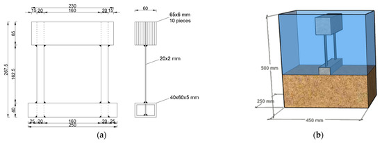
Figure 1.
(a) Physical experimental model, (b) sand container.
The model was excited by a time-varying sinusoidal waveform (sine sweep function), which is presented in Figure 2c in the out-of-plane direction to determine its fundamental frequency. The model structure was tested for two support cases. First, the tested model was attached directly to the shaking table platform (Figure 2a). Second, the examined model was placed on a layer of compacted sand (Figure 2b) embedded in sand container (Figure 2d marked number 1) The measured experimental data were later used for the calibration of the numerical models, specifically for the parameters regarding SSI.
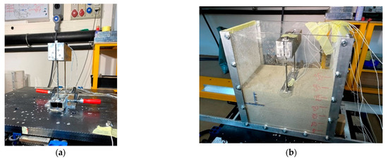
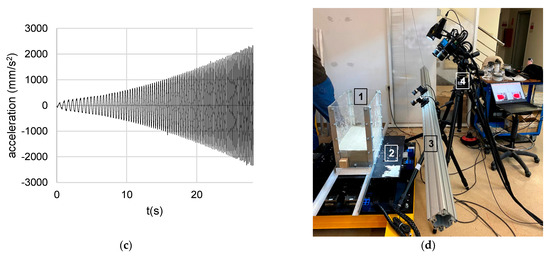
Figure 2.
Physical model tested as fixed at the base (a), and founded on the sand bed (b), excitation function (c) and testing setup (d).
The River Drava sand used in this experiment represents uniformly graded sand. The mean grain size diameter (D50) is approximately 0.28 mm, and the effective grain diameter (D10) is 0.18 mm. The coefficient of curvature, Cu, is approximately 1.67. The minimum void ratio (emin) and maximum void ratio (emax) of the tested sand are 0.627 and 0.951, respectively. The friction angle was measured to be 33.75°. Completely dry sand was embedded in 5-cm-thick layers. After the installation of each layer, the seismic platform was activated in order to compact the sand layers. The mass of sand for each placed layer was determined by weighing before installation in the container, and the volume of installed sand was determined after compacting. The mass and volume measured in this way were used to determine the density of 1510 kg/m3.
2.3. Test Setup
A large number of measuring instruments were used for the purpose of testing. Accelerometers were placed on top of the structure model, on the foundation and on the shaking table. Accelerometers were used to obtain shear wave velocity in sand and to determine the period of vibration of the model before the dynamic test was conducted. The accelerometers had a sensitivity of 4.91 mV/g. Displacements were measured with two optical measuring systems. The first system (marked with number 4 in Figure 2d) was used to measure displacements of the structural model, and the other for measuring the displacement of the soil model (marked with number 3 in Figure 2d). The dynamic response of the structure model was recorded by an optical 3D displacement and deformation measurement system GOM Aramis and Pontos with frequency recording up to 160 fps in full resolution. The measuring volume covered by the system is 2000 mm × 1000 mm × 500 mm. Soil displacement was measured using a GOM Aramis 12 M noncontact optical 3D displacement and deformation measurement system with 12 mm focal length lenses and a speed of 3 images per second.
Dynamic tests were carried out by applying dynamic ground excitation via the Quanser ST-III earthquake platform (marked with number 2 in Figure 2d), which has dimensions of 70 cm × 70 cm and the possibility of a maximum acceleration of 1 g in both directions with a maximum load of 120 kg.
2.4. Numerical Models
Experimental results from the experiment presented in the previous chapter were used to develop, calibrate and validate numerical models used for realistic shallow foundation structures founded on compliant soils. This research is a continuation of the research [48] that the authors conducted earlier using data from TRISEE experimental research [53,54] conducted in Italy.
The SAP2000 [55] software was used to create numerical models. This software was chosen because it enables effective numerical modelling of the nonlinear behaviour of the structure and is also effective in modelling the effects of soil-structure interaction under seismic loading [43,56,57,58].
Soil modelling is a very complex task since the soil is not an engineered material, and a quantitative description of its mechanical and chemical interactions requires a large set of stochastic parameters. Numerous geotechnical computer programmes and modelling approaches provide very realistic assessments of soil behaviour [45,59,60], but they require relatively large sets of input data and often complex and time-consuming numerical calculations. Taking this into account and aiming to keep soil models as simple as possible, the Winkler soil model [61] was chosen, which simulates soil behaviour using springs. The authors used nonlinear springs following the principles described in the following chapter.
To create a Winkler soil model, it is initially necessary to define the stiffness of the soil. A study [62] was conducted to decide on the selection of a model to be used in further research. Based on the aforementioned study, the soil model proposed in [63] was selected, where expressions for the calculation of the stiffness of translational and rotational springs were given. These expressions were also studied by Brandis et al. [48], where good agreement between the numerical calculation results and the experimentally obtained results was observed. Further research on the models tested with dynamic loads replaced the springs’ stiffness calculation according to Pais and Kauesl [64], which is very similar to the expressions used earlier [63] but also provides expressions for adjusting stiffness for dynamic loads and buried foundations. Expression (1)–(3) describe the stiffness of the underlying soil under the foundation, while Expression (4)–(6) refer to the adjustment of stiffness in the case of an embedded foundation [63]:
The symbols in Equations (1)–(6) indicate: kz,sur is the soil stiffness in the vertical z direction, ky,sur is the soil stiffness in the horizontal y direction, kx,sur is the soil stiffness in the horizontal x direction, G is the shear modulus, B represents half the width of the foundation, L represents half the length of the foundation, D is the depth of the lower surface of the foundation, ν is the Poisson’s ratio. The positions of the foundation coordinate system and the geometric characteristics of the foundation are shown in Figure 3.
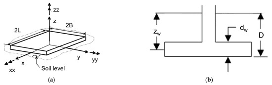
Figure 3.
Foundation geometry: axonometry (a) and cross-section (b) [63] (edited by the authors).
Nonlinear link elements in the computer programme SAP2000 [55] were used to model soil behaviour in the vertical direction. These elements require information regarding the stiffness, force-displacement relationship and type of hysteretic behaviour of the soil. The force-displacement curve was adopted according to the recommendation given by Rees and Van Imp [65], which is primarily defined for modelling the soil around the piles. The curve describing the behaviour of the soil is shown in Figure 4a, and the following expressions were used to calculate the points at which a change in stiffness occurs [65,66]:

Figure 4.
P-y curve created according to Reese and Van Impe [65] (a) and force-displacement curve used for horizontal link elements (b).
The symbols in Equations (7)–(10) indicate: b is the foundation width, z is the foundation depth, γ is the specific weight of the soil and φ is the internal friction angle of the soil.
All other parameters, such as α, β, k0, ka, are determined using existing soil information [66], while the quantities (), () are read from the diagram given in [66] as well as k_py which is read depending on the type and compaction of the soil [65].
To describe the hysteretic behaviour of the soil, Takeda’s model [67] was chosen. Takeda’s model was primarily developed for modelling the response of reinforced concrete structures, but it can also be used for nonlinear soil modelling [68].
To model the behaviour of the soil in the horizontal direction, the bilinear elastic link elements were used, where the friction force Ffr on the contact surface between the foundation and the soil was used as the limit value of proportionality (Figure 4b). The friction force was calculated as the product of the total weight of the model and the coefficient of friction. The value of the coefficient of friction was determined by calculation from the experimentally obtained angle of internal friction of sand and it was equal to μ = 0.50.
Given that the physical model was relatively small, its numerical model needed to be created on an enlarged scale (10:1). As all the soil models were developed for real-size structures, it is not possible to implement them directly in the case of the scale model. Therefore, for the purpose of numerical modelling, a scaled version of the experimental model was considered by applying scaling coefficients as suggested in [45,59,69]. Table 2 gives the expressions and scaling coefficients. A scaling factor of λ = 10 was chosen, so that the final dimensions of the enlarged model would more realistically reflect the dimensions of the real buildings.
Table 2.
Considered scaling coefficients.
Structural members were modelled with 3D finite beam elements, considering their cross-sectional (Table 3) and material properties. For the rigid beam, a rectangular solid steel element was used. To realistically describe the behaviour of the columns that were fixed to the beam elements at their ends, the “offset end” function was used.
Table 3.
Numerical model dimensions.
2.5. Comparison of Experimental and Numerical Results
Firstly, the results of the modal analysis were compared. For the fixed-based numerical model, two predominant vibration modes were observed: the first was in the direction perpendicular to the plane of the model (T1 = 1.51 s), and the second was torsional (T2 = 0.61 s). The measured values of the periods of vibration of the experimental fixed-base model that were scaled considering the scaling coefficient were T1 = 1.52 s and T2 = 0.60 s. Moreover, by observing the free vibrations of the model after the dynamic load test, the damping of the fixed-base physical model was measured and calculated at 0.66%, which was also used in the numerical model.
Damping was determined from the free oscillations measured after the sine sweep excitation had stopped. The record is first smoothed, and then Expression 11 [70] is used.
If Expression (11) is observed, j is the number of waves between the observed chosen points of free oscillations, ui is the displacement at the beginning of the observation and ui+j is the displacement at the end.
Secondly, a time-history analysis was conducted on the fixed-base numerical model with the sine sweep function as the input. Figure 5a shows the lateral displacements of the top beam. For comparison, the lateral displacements from the shake table test of the scaled model subjected to the same time-history input are also presented. Additionally, the floor response spectra are shown and compared in Figure 5b. In both comparisons shown in Figure 5, good agreement between the experimental and numerical results is observed.
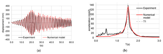
Figure 5.
Fixed-base results for sine sweep excitation: (a) displacement of the top beam and (b) floor spectra.
In the next phase, the numerical model of the structure was upgraded to include the foundation and the soil model, by adding vertical links that were distributed along the foundation at equal intervals, as shown in Figure 6a. The links were connected to the foundation model via massless rigid cantilever finite elements (Figure 6a). The length of rigid finite elements corresponded to half of the width of the foundation. To connect the columns with the foundation beam and keep the realistic geometry of the model, an additional massless rigid element was added at the bottom of the column.
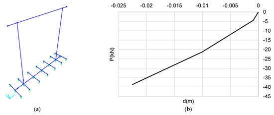
Figure 6.
Numerical model of the SSI case (a) and force-displacement curve for the soil links (b).
The model amounted to a total of 21 vertical and 7 horizontal link elements calculated using soil properties given in Table 4. The inelastic properties of the vertical links were assigned in terms of the P-y curve (Figure 6b), and the vertical stiffness was equal to kz = 82,288.7 kN/m.
Table 4.
Soil properties for definition of P-y curve.
To the horizontal links, a stiffness of ky = 277,745.6 kN/m was assigned, and the limiting value of the friction force FTR, at which a change in stiffness occurs, was equal to 7.58 kN. A kinematic hysteresis loop was considered for the energy dissipation of horizontal links.
Two predominant periods of vibration of the model, equal to T1 = 1.51 s and T2 = 0.61 s were observed. The measured values of the periods of vibration of the experimental SSI model that were scaled considering the scaling coefficient were T1 = 1.54 s and T2 = 0.38 s.
Certain differences in the vibration period of the numerical and enlarged physical models were evident, and the beam displacement results showed a satisfactory match. In the case of the physical model SSI, a large change in the vibration period of the system was observed during the test due to the changes created in the sand by compaction, which is not possible to model and describe with a numerical model of this kind.
The numerical model of the soil-foundation-structure system was later excited by the same time records as the fixed base model. The response of the experimentally tested and numerical model was compared by comparing the horizontal displacements of the top of the beam (Figure 7a) and the floor spectra (Figure 7b).

Figure 7.
SSI model results for sine sweep excitation: (a) displacement of the top beam and (b) floor spectra.
A comparison of the displacements at the top of the beam during loading with the time-history loading gives a satisfactory match, which is shown in Figure 7a. For the numerical models, damping in the amount of 4.66% was used. The increase in damping compared to the fixed-base physical model occurs due to the influence of dry sand under the structure. The increase in damping was also observed by other researchers [39,71,72,73].
The comparison between the numerical and scaled results of the experimental model is shown in Table 5. In terms of the floor spectrum, they were compared for the first 11.3 s of excitation. Up to this point in the dynamic loading, there has been no pronounced change in the properties of the foundation soil, and it is possible to compare the floor spectra. For this range, the numerical model shows good agreement with the physical model. Changes in the underlying soil occur due to the displacements of the scaled model and vibrations from the seismic platform, which cause additional soil compaction and consequently changes in the soil’s dynamic properties over time. These changes cannot be properly accounted for by the considered numerical model.
Table 5.
Comparison between the scaled experimental results and numerical results.
3. Proposed Step by Step Procedure for Conducting the N2 Method with SSI
This chapter provides a proposal for the implementation of soil-structure interaction effects into the N2 method. An algorithm shows the necessary steps to include SSI effects in the N2 method.
The advantage of the new application of the N2 method, compared to the conventional N2 method, can be seen in the fact that the proposed extension allows insight not only into the inelastic behaviour of the load-bearing elements of the structure, but also provides insight into the behaviour of the foundation soil. It is also possible to obtain information on the rotation of the foundation and the structure at different acceleration levels. The biggest difference between the proposed new extension of the N2 method and its classical form manifests in the numerical modelling of the structural system and its supporting system. Initially, the N2 method was developed without consideration of the compliance of the soil under the building’s foundations. For the purpose of implementing the new application of the N2 method, it is necessary to design the foundations following the procedures from Eurocode 7—Part 1 [74].
With all previous information considered, the following steps, also presented in Figure 8, should be followed to implement the N2 method for soil-structure systems:

Figure 8.
Algorithm for implementing the new application of the N2 method on soil-structure systems.
- Calculation and design of the structure and its foundation. Calculation of soil stiffness, force-deformation relationship and definition of the hysteresis model so that the soil and foundation can be included in the numerical analysis. The stiffness can be determined according to NIST [63], the force-deformation relationship as it is used for the design of piles [65], and the hysteresis should be chosen to match the soil hysteresis loop as closely as possible.
- Creation of an inelastic numerical model with the addition of foundations.
- Definition of the vertical distribution of the lateral loads based on the mode of vibration corresponding to the observed direction of the pushover analysis. The mass of the foundation level should be included as an additional floor of the structure.
- Pushover analysis to obtain the capacity curve in the force-displacement form for the MDOF system.
- Idealization of the capacity curve and transformation of the idealised capacity curve into the acceleration-displacement form.
- Definition of the required response spectrum using data from the foundation soil and PGA with the appropriate return period. The spectrum defined in this way is given in an acceleration-period format.
- Transformation of the response spectrum into acceleration-displacement form.
- Definition of the inelastic response spectrum.
- Determining the intersection point of the curves from steps 5 and 8, which indicates the target displacement. If the intersection is located on the elastic branch of the capacity curve, the elastic response spectrum can be used, while otherwise it is necessary to use the inelastic response spectrum.
- Transformation of the target displacement for the corresponding MDOF system.
- Conducting the pushover analysis of the numerical model up to the value of the target displacement for the purposes of designing or assessing structural damage.
4. Nonlinear Static Analysis—Case Study with Soil-Structure Interaction
4.1. Examined Case Study Building
In the second part of the study, the seismic response of a 5-story steel building was investigated using 3D finite element numerical simulation. A fixed-base (FB) analysis as well as soil–structural interaction (SSI) were considered in this research. The selected case study building was designed in accordance with Eurocode 8—Part 1 for the FB case [75,76]. The building consists of three moment-resisting frames with 9-m bay spans in the longitudinal direction (X-direction) and braced frames with 9-m bay spans in the transverse direction (Y-direction), where diagonal bracing was installed on the outermost frames (Figure 9). All elements were composed of steel-grade S275JR. The structure was rock-founded, which corresponds to soil category A according to Eurocode 8—Part 1 [4]. Peak ground acceleration (PGA) used for building design was equal to 0.30 g. The design of the building was created following EN Eurocodes.
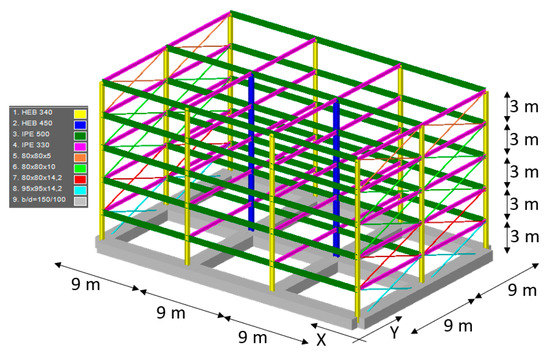
Figure 9.
Analysed steel frame building.
The structure was initially designed for the gravity and wind loading scenarios. The structure’s self-weight and the weight of the floor finishing, both equal to 2.00 kN/m2, were considered in addition to an imposed load of 3.00 kN/m2. Discrete loads were assigned to the joints in the form of concentrated forces. A seismic design was considered by using the equivalent forces method. Furthermore, the adopted behaviour factor was 6.5 and refers to multi-story moment frames for which high ductility is proposed. The participating seismic mass of the building consisted of 100% permanent and 30% variable load. Numerical models were created using the software SAP2000 v21.0.2 [55].
Material nonlinearity in accordance with Eurocode 8—Part 3 [77] was considered in the form of lumped plasticity by employing plastic hinges at the endpoints of the columns and beams. Plastic hinges were modelled with a trilinear moment-rotation relationship, while the yield moment (My) and plastic moment (Mp) were determined for each section separately and were manually assigned to the elements of the numerical model.
Table 6 shows the values of My and Mp, together with the corresponding yield rotation θy and rotation at full plastification θp. It was determined that the axial force in the columns does not affect the load capacity (N_Ed/N_cr < 4%), therefore, pure biaxial bending was considered. The building was designed according to the principles of capacity design. Therefore, the plastic hinges first appear in the beams, followed by plastic hinges in the columns.
Table 6.
Plastic hinges properties.
In diagonal bracing elements, the plastic hinges followed compressive and tensile limits for axial tensile displacements Δt and axial compressive displacements Δc.
Rigid diaphragms were assigned to each floor of the structure, and in the centre of gravity of each floor, additional nodes were added to which lateral forces for pushover analysis were applied.
To study the effects of SSI on the numerical model of the building, RC foundation strips were designed and added to the model. It was assumed that the building foundation soil corresponded to the soil considered in the experimental campaign presented in Section 2. Therefore, the soil layer under the foundations was modelled using data from Table 4. The foundations were designed following guidelines from Eurocode 7 [74] and the Croatian National Annex [78], which imply the use of design approach number 3 from Eurocode 7 [74]. The mass of each floor was 290 t, while the mass of the strip foundations was 976 t.
The designed foundation strips were 1.50 m wide and 1.00 m deep. The strips formed a foundation grid, connecting all columns in both the X and Y directions, respectively. The soil was modelled using three link elements under each column. The properties of every link are given separately in Table 7 and Table 8 and Figure 10.
Table 7.
Link elements—stiffness.
Table 8.
Properties of horizontal link element.

Figure 10.
Force-deformation (P-y) relation assigned to corner column, edge column and middle column.
The governing modes of vibration of the fixed-base model are T1 = 1.11 s (X-direction), T2 = 0.53 s (Y-direction) and T3 = 0.41 s (torsional), while for the SSI numerical model the governing modes of vibration are T1 = 1.13 s (X-direction), T2 = 0.57 s (Y-direction) and T3 = 0.44 s (torsional).
4.2. Pushover Analysis and Target Displacement Based on the N2 Method
The pushover analysis was conducted for both directions of the building, by considering the normalised horizontal displacements corresponding to the first mode of vibration and the modal masses of each floor (Figure 11 and Table 9). The capacity curve for both governing directions is presented in Figure 11.

Figure 11.
Vertical distribution of lateral forces for pushover analysis.
Table 9.
Normalized values of lateral pushover forces.
In the same manner, the lateral forces for the SSI model were calculated and are shown in Figure 11 and Table 9. For the SSI case, the capacity curves (Figure 12b) exhibit slightly lower stiffness, when compared to the fixed base case (Figure 12a). Moreover, a slightly higher bearing capacity is also achieved due to the inclusion of the foundation and soil in the calculation.

Figure 12.
Capacity curves for the fixed base model (a) SSI model for X and Y directions (b).
The target displacement, also called the seismic demand displacement (dD), which represents the displacement of the top floor in a seismic event, was determined by using the N2 method. Two levels of the peak ground acceleration (PGA) were considered, namely PGA = 0.215 g, for a return period of 475 years and PGA = 0.10 g, for a return period of 95 years.
The considered foundation soil is classified as category E in Eurocode 8—Part 1 [4]. Soils in this category are characterised by a pronounced change in stiffness with depth, which can be classified into almost all soil models used in experimental research on the effects of soil-structure interaction [47,79,80,81]. Generally, experimental research on the effects of soil-structure interaction carried out on seismic platforms consists of a soil container and a soil model, in which case the soil model has significantly lower stiffness than the stiffness of the suspended container [46,47].
The capacity curves obtained within the pushover analysis were originally given as force-displacement ratios. Since the N2 method considers the inelastic spectrum in the acceleration–displacement format, the ordinate of the capacity curve (the base-shear force) needs to be divided by the value of the participating seismic mass of the structure. After the capacity curve in the said format is defined, it is also necessary to define the corresponding inelastic response spectrum based on Eurocode 8—Part 1 [4] in this format. From the intersection of the capacity curve and the inelastic response spectrum, the dD can be obtained, which is the result of the N2 method.
4.3. Comparison between the FB and SSI Models
By comparing the periods of vibration of the FB model and the SSI model, an increase in the period of vibration of roughly 3% was observed for the models based on a flexible support. The comparison of target displacements is shown in Table 10. An increase in the target displacement of approximately 7% for the SSI model was observed.
Table 10.
Target displacements at a PGA level of 0.10 g and 0.215 g.
The capacity curves are shown in Figure 13. It is possible to observe a slight difference between the stiffness and the bearing capacity for both observed cases of supports. Fixed base models have higher stiffness than models on the soil due to deformability of the soil itself when subjecting the soil-structure system to lateral loading. It should be pointed out that the apparent higher loadbearing capacity of the SSI model, stems from the coupled system comprising of the superstructure and the foundation layer and not from the increase in the capacity of the structure itself, since an additional lateral force is included at foundation level.

Figure 13.
Capacity curves (a) full range and (b) only linear-elastic part.
To further analyse the effects of SSI, a comparison of inter-story drifts was also conducted. Although it can be concluded that the target displacement of the SSI model is larger, this does not necessarily mean an increase in inter-story drifts, as the soil is also deformable and contributes to the overall response of the structure. The values of the limit inter-story drifts for the direction of the moment frame (X-direction) and the braced frame (Y-direction) are shown in Table 11. The limit values of the story-drifts in the moment-resisting frames were defined through the chord rotations of the columns, while in the braced frame the limit elongation of the brace in tension was used to determine the limit value of the story drift. A more detailed procedure and selection of threshold values are given in the literature [77,82]. According to the adopted Eurocode norm [77], limit inter-story drifts should be checked for: (i) a seismic return period of 475 years, i.e., the limit state of significant damage (SD), and (ii) the limit state of damage limitation (DL), which corresponds to a return period of 95 years.
Table 11.
Limit values of inter-story drifts.
Figure 14a,b show the inter-story drifts for the target displacement cases shown in Table 10. More specifically, the inter-story drifts for the corresponding one of the two considered PGA values are shown. It can be concluded that generally, the inter-story drifts for the SSI models are larger than those of the FB models in the first story. Thus, for SSI models, a reduction in the inter-story drifts was observed at the ground floor level, while the middle floors mostly had either the same or greater inter-story drifts when compared to the FB model. It is important to note that none of the models resulted in inter-story drifts greater than the limit values, but displacement changes should be taken into account because it is not possible to conclude unambiguously whether including soil in the calculation results in a reduction or increase in inter-story drifts.
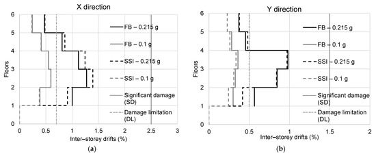
Figure 14.
Inter-story drifts: (a) X-direction, (b) Y-direction.
In the observed case, the level of inter-story drift is lower on the ground floor for the model if the flexibility of the foundation soil is considered, but the inter-story displacements are greater by 10% for higher floors (Table 12). This is important to keep in mind when designing buildings, especially when considering the impact on partition (masonry) walls and installations.
Table 12.
Comparison of inter-story drifts.
Moreover, a comparison based on the seismic return periods shown in Figure 15 was also carried out for each calculated target displacement. By comparing the corresponding pairs of data for the SSI and FB models for the same PGA, a trend in the increase in the return period was observed for SSI models for the structure to reach a certain damage grade. For some cases, this increase is less pronounced. Thus, in the case of the Y-direction and the PGA = 0.215 g, the increase was approximately 1.5%, while in the X-direction and the PGA = 0.215 g, the increase in the return period was approximately 30%.

Figure 15.
Return periods for all cases according to the N2 method shown on a logarithmic scale.
5. Nonlinear Time-History Analysis
5.1. Input Data and Selection of Ground-Motion Records
The validation of the results obtained by the pushover analysis was conducted by means of nonlinear time-history analysis since it is well known that this type of analysis gives the most accurate response estimation of a structure under seismic excitations [83]. This method can reproduce the inelastic dynamic behaviour of structures with a high degree of accuracy and is, therefore, often implemented for validation purposes [84].
An important step in any time-history analysis is always the selection of input ground-motion records. In general, time-history records of ground acceleration can be recorded during real earthquake events or are artificially generated. Building codes impose the minimum number of records that must be used during the calculation and provide criteria for compliance of the records with the required seismic spectra. For example, Eurocode 8—Part 1 [4] requires at least three records to assess the seismic response of the structure by means of a time-history analysis. However, it is often the case in studies [85,86], that at least seven records are considered necessary to minimise the dispersion of results. By using a larger number of records, it is possible to interpret the average values of results, and not only their maximum values.
The computer software REXEL [87] was used to select appropriate ground-motion records. This software is publicly available and enables the selection of seismic records from the European Strong Motion Database [88] that correspond to the defined elastic spectrum in European building codes. Seven earthquake records were selected by considering the site class and properties of the response spectra used for the N2 method. Each record was later modified by using the computer software SYNTH [89], to match the characteristics of the required response spectrum even more closely (Figure 16). In this way, a total of 14 ground-motion records were obtained, which were used during the nonlinear time-history calculation. All records were initially scaled to PGA = 0.215 g, which corresponds to a seismic return period of 475 years. Additionally, the records were also scaled to PGA = 0.10 g to correspond to a seismic return period of 95 years.

Figure 16.
Elastic demand spectrum and average spectrum according to REXEL and SYNTH (TR = 475 yrs).
It can be seen from Figure 16 that the overlap of the average response spectra of the REXEL and SYNTH records is in good agreement with the code-based elastic spectrum, especially in the areas of the periods of vibration related to the observed structure. This is important because it significantly affects the response of the structure during the numerical calculation.
Rayleigh type damping was assumed by considering the recommendations for steel structures given by Satake and co-authors [90]. The considered damping values are presented in Table 13. Additionally, hysteretic damping was included in the inelastic response of the plastic hinges, where the kinematic hysteresis loop was considered.
Table 13.
Considered viscous Rayleigh damping values.
5.2. Analysis Results and Comparison with N2 Results
The validity of the applicability of the N2 method on the SSI model was checked by comparing the results with the results of the nonlinear time-history analyses. Target displacement was determined graphically, as it is shown for certain cases in Figure 17a for FB and Figure 17b for SSI for a PGA value of 0.215 g. The graphical representation shows values of target displacement for an equivalent single degree of freedom system (marked with *), which need to be transformed to values for building using the transformation factor Γ. Transformation factors are given in Table 14. The target displacement that was calculated by the means of the N2 method in Section 4 is compared in Table 15 with the average value of the largest peak displacement obtained by nonlinear dynamic analysis. Comparisons were made for both observed PGA values, which are shown in Table 15. By comparing these values, it is possible to observe that the target displacement mostly exceeded the lower PGA, while the displacements for the dynamic and N2 method analyses are very similar for the higher PGA.

Figure 17.
Graphical representation of the N2 method for PGA 0.215 g and for FB (a) and SSI (b).
Table 14.
Values of transformation factors.
Table 15.
Comparison of target displacements and average maximal displacements.
Furthermore, inter-story drifts were also observed, which were compared with the limit values defined by the Eurocode 8—Part 3 [77].
For PGA = 0.215 g, it is possible to observe a decrease in inter-story drifts for the SSI model on the ground floor (Figure 18a), while in the case of higher floors, an increase in inter-story drifts was observed. This trend is repeated for the results obtained by the N2 method and both dynamic analyses, but with slightly different values.
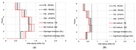
Figure 18.
Comparison of inter-story drifts for: (a) X-direction, PGA = 0.215 g and (b) X-direction, PGA = 0.10 g.
For PGA = 0.10 g, a similar shape of inter-story drifts was obtained (Figure 18b), implying more pronounced displacements of the second and third storeys and very small drift values on the ground floor. In this case, it is not possible to discern the results of all performed analyses in the same way because, for example, a slight decrease in the story drift was observed for both dynamic analyses, while the results of the N2 method showed an increase in the inter-story drift for the SSI model. Observing only these results, it is not possible to conclude whether the inclusion of SSI diminishes or amplifies the seismic load.
For the braced frame (Figure 19), shear behaviour is expected in the case of lateral loading. Therefore, a reduction in inter-story drifts at the ground floor level was observed for SSI models at both PGA levels. Generally, the N2 method gives larger inter-story drifts, when compared to time-history analyses of the FB model. For all storeys above the ground floor, the dynamic analysis of the soil-structure system forecast a decrease in inter-story drifts, while the results of the N2 method showed an increase in the drifts. The shape of the story-drifts with respect to the height of the building is similar in all analysed models, with more pronounced values of drifts in the higher storeys.

Figure 19.
Comparison of inter-story drifts for: (a) Y-direction, PGA = 0.215 g and (b) Y-direction, PGA = 0.10 g.
6. Conclusions
The main goal of this research is to extend the applicability of the N2 method to soil-structure systems. One of the advantages of the N2 method is that it can be used as a graphical method to obtain the target displacement for a selected PGA. The method can be used when designing new buildings or for assessing the seismic performance of existing buildings.
The main hypothesis of this research states that the application of N2 methods is possible for soil-structure systems. It is built on the assumption that the soil can be seen as a damper under the structure, which indicates a coupled system. It is assumed that the coupled system oscillates predominantly in the first eigenmode, which is also the main assumption of the N2 method. This assumption already made it possible to extend the N2 method for the purposes of assessing the behaviour of buildings with base-isolation. These assumptions led to the idea of using the N2 method for evaluating the behaviour of soil-structure systems, which behave in a similar manner. The hypothesis was verified and tested with the support of the results of experimental research conducted on scaled models that were fixed into the ground or founded on compliant soil. Additionally, the experiments have been supported by a numerical study on a 3D spatial model of a steel-framed building.
The new application of the N2 method requires the design and modelling of the foundation as well as the modelling of the soil. For the numerical modelling of the soil, it is necessary to use nonlinear springs, the definition of the force-displacement relationship for the observed foundation, and the hysteric behaviour that includes the dissipation of seismic energy in the soil.
The results obtained by this new application of the N2 method, validated by nonlinear dynamic time-history analysis, show good agreement and prognosis when this method is used for buildings on compliant soils. Overall, it was observed that a decrease in the inter-story drifts appears at ground level of the building while the value of the inter-story drift is kept the same or is larger at higher storeys of the building.
The new application of the method has two additional steps compared to classic N2 method: (i) design of foundations and (ii) definition of the soil numerical model. In order to define the soil numerical model, it is necessary to know the geometry of the foundation, density of the soil, shear modulus, hysteresis shape and poisons ratio.
Future work on this topic should focus on how different types of buildings and building typologies, as well as irregularities in the structural systems, are affected by this approach. The approach can be further developed to also include liquefaction effects and the effects of SSI on the building collapse, as well as innovative approaches that, for instance, consider structure–soil–structure dynamic interaction with multiple adjacent buildings in dense urban areas.
Author Contributions
Conceptualization, A.B., I.K. and S.P.; methodology, A.B., I.K. and S.P.; software, A.B.; investigation, A.B.; writing—original draft preparation, A.B.; writing—review and editing, I.K. and S.P. All authors have read and agreed to the published version of the manuscript.
Funding
This work was carried out within the framework of the SYNERGY research project and supported by grant No. IZIP_A_02 by Josip Juraj Strossmayer, University of Osijek, Faculty of Civil Engineering and Architecture, Croatia, and co-funded by the Slovenian Research Agency (ARRS), grant number P5-0068. The support of both institutions is gratefully acknowledged.
Institutional Review Board Statement
Not applicable.
Informed Consent Statement
Not applicable.
Data Availability Statement
Not applicable.
Acknowledgments
The experimental activity presented herein was part of the SYNERGY research project funded by Josip Juraj Strossmayer University of Osijek, Faculty of Civil Engineering and Architecture, Croatia.
Conflicts of Interest
The authors declare no conflict of interest.
References
- Lou, M.; Wang, H.; Chen, X.; Zhai, Y. Structure–soil–structure interaction: Literature review. Soil Dyn. Earthq. Eng. 2011, 31, 1724–1731. [Google Scholar] [CrossRef]
- Khalil, L.; Sadek, M.; Shahrour, I. Influence of the soil–structure interaction on the fundamental period of buildings. Earthq. Eng. Struct. Dyn. 2007, 36, 2445–2453. [Google Scholar] [CrossRef]
- Fiamingo, A.; Bosco, M.; Massimino, M.R. The role of soil in structure response of a building damaged by the 26 December 2018 earthquake in Italy. J. Rock Mech. Geotech. Eng. 2022, in press. [Google Scholar] [CrossRef]
- CEN. Eurocode 8: Design of Structures for Earthquake Resistance—Part 1: General Rules, Seismic Actions and Rules for Buildings, Design Code EN 1998-1; European Committee for Standardisation: Brussels, Belgium, 2005. [Google Scholar]
- Fajfar, P. A Nonlinear Analysis Method for Performance-Based Seismic Design. Earthq. Spectra 2000, 16, 573–592. [Google Scholar] [CrossRef]
- Sullivan, T.J.; Welch, D.P.; Calvi, G.M. Simplified seismic performance assessment and implications for seismic design. Earthq. Eng. Eng. Vib. 2014, 13, 95–122. [Google Scholar] [CrossRef]
- Čaušević, M.; Zehentner, E. Nelinearni seizmički proračun konstrukcija prema normi EN 1998-1: 2004. Građevinar 2007, 59, 767–777. [Google Scholar]
- Bhatt, C.; Bento, R. Assessing the seismic response of existing RC buildings using the extended N2 method. Bull. Earthq. Eng. 2011, 9, 1183–1201. [Google Scholar] [CrossRef]
- Fajfar, P.; Fischinger, M.; Isaković, T. Metoda procjene seizmičkog ponašanja zgrada i mostova. Građevinar 2000, 52, 663–671. [Google Scholar]
- Krolo, P.; Čaušević, M.; Bulić, M. The extended N2 method in seismic design of steel frames considering semi-rigid joints. In Proceedings of the Second European Conference on Earthquake Engineering, İstanbul, Turkey, 25–29 August 2014; pp. 1–10. [Google Scholar]
- Koren, D.; Kilar, V. The applicability of the N2 method to the estimation of torsional effects in asymmetric base-isolated buildings. Earthq. Eng. Struct. Dyn. 2011, 40, 867–886. [Google Scholar] [CrossRef]
- Kilar, V.; Koren, D. Simplified inelastic seismic analysis of base-isolated structures using the N2 method. Earthq. Eng. Struct. Dyn. 2010, 39, 967–989. [Google Scholar] [CrossRef]
- Kilar, V.; Koren, D. Usability of Pushover Analysis for Asymmetric Base-Isolated Buildings; COMPDYN: Corfu, Greece, 2011. [Google Scholar]
- Kilar, V.; Petrovčič, S.; Šilih, S.; Koren, D. Financial aspects of a seismic base isolation system for a steel high-rack structure. Inf. Construcción 2013, 65, 533–543. [Google Scholar] [CrossRef]
- Krawinkler, H. Pushover analysis: Why, how, when, and when not to use it. In Proceedings of the 65th Annual Convention of the Structural Engineers Association of California, Maui, HI, USA, 1–6 October 1996; pp. 17–36. [Google Scholar]
- Ruggieri, S.; Uva, G. Accounting for the Spatial Variability of Seismic Motion in the Pushover Analysis of Regular and Irregular RC Buildings in the New Italian Building Code. Buildings 2020, 10, 177. [Google Scholar] [CrossRef]
- Fujii, K. Assessment of pushover-based method to a building with bidirectional setback. Earthq. Struct. 2016, 11, 421–443. [Google Scholar] [CrossRef]
- Fischinger, P.F.M. N2—A method for non-linear seismic analysis of regular buildings. In Proceedings of the Ninth World Conference in Earthquake Engineering, Tokyo, Japan, 1 August 1988. [Google Scholar]
- Kilar, V.; Fajfar, P. Simple push-over analysis of asymmetric buildings. Earthq. Eng. Struct. Dyn. 1997, 26, 233–249. [Google Scholar] [CrossRef]
- Gaspersic, P.; Fajfar, P.; Fischinger, M. An approximate method for seismic damage analysis of buildings. In Proceedings of the 10th World Conference on Earthquake Engineering, Madrid, Spain, 19–24 July 1992; pp. 19–24. [Google Scholar]
- Fajfar, P.; Gašperšič, P. The N2 method for the seismic damage analysis of RC buildings. Earthq. Eng. Struct. Dyn. 1996, 25, 31–46. [Google Scholar] [CrossRef]
- Mitrović, S.; Čaušević, M. Nelinearni statički seizmički proračuni konstrukcija. Građevinar 2009, 61, 521–531. [Google Scholar]
- Kim, G.-W.; Song, J.-G. Lateral Load Distribution Factor for Modal Pushover Analysis. In Proceedings of the Earthquake Engineering Society of Korea Conference; Earthquake Engineering Society of Korea: Seoul, Republic of Korea, 2005; pp. 236–243. [Google Scholar]
- Winkler, E. Die Lehre von der Elasticitaet und Festigkeit: Mit Besonderer Rücksicht auf ihre Anwendung in der Technik, für Polytechnische Schulen, Bauakademien, Ingenieure, Maschinenbauer, Architecten, etc.; H. Dominicus, 1867. [Google Scholar]
- Cavalieri, F.; Correia, A.A.; Crowley, H.; Pinho, R. Dynamic soil-structure interaction models for fragility characterisation of buildings with shallow foundations. Soil Dyn. Earthq. Eng. 2020, 132, 106004. [Google Scholar] [CrossRef]
- Burnwal, M.L.; Raychowdhury, P. A Comparative Study on Predictive Capability of Different SSI Models. In Seismic Design and Performance: Select Proceedings of 7th ICRAGEE 2020; Springer: Singapore, 2021; Volume 120, pp. 193–205. [Google Scholar]
- Crouse, C.; Hushmand, B.; Martin, G.R. Dynamic soil–structure interaction of a single-span bridge. Earthq. Eng. Struct. Dyn. 1987, 15, 711–729. [Google Scholar] [CrossRef]
- Aldaikh, H.; Alexander, N.A.; Ibraim, E.; Oddbjornsson, O. Two dimensional numerical and experimental models for the study of structure–soil–structure interaction involving three buildings. Comput. Struct. 2015, 150, 79–91. [Google Scholar] [CrossRef]
- Kocak, S.; Mengi, Y. A simple soil–structure interaction model. Appl. Math. Model. 2000, 24, 607–635. [Google Scholar] [CrossRef]
- Dhadse, G.D.; Ramtekkar, G.; Bhatt, G. Finite Element Modeling of Soil Structure Interaction System with Interface: A Review. Arch. Comput. Methods Eng. 2020, 28, 3415–3432. [Google Scholar] [CrossRef]
- Brinkgreve, R.B. Selection of soil models and parameters for geotechnical engineering application. In Soil Constitutive Models: Evaluation, Selection, and Calibration; Delft University of Technology: Delft, The Netherlands, 2005; pp. 69–98. [Google Scholar]
- Lopez-Caballero, F.; Farahmand-Razavi, A.M. Numerical simulation of liquefaction effects on seismic SSI. Soil Dyn. Earthq. Eng. 2008, 28, 85–98. [Google Scholar] [CrossRef]
- Forcellini, D. Soil-structure interaction analyses of shallow-founded structures on a potential-liquefiable soil deposit. Soil Dyn. Earthq. Eng. 2020, 133, 106108. [Google Scholar] [CrossRef]
- Forcellini, D. Analytical fragility curves of shallow-founded structures subjected to Soil-Structure Interaction (SSI) effects. Soil Dyn. Earthq. Eng. 2021, 141, 106487. [Google Scholar] [CrossRef]
- Forcellini, D. Seismic fragility for a masonry-infilled RC (MIRC) building subjected to liquefaction. Appl. Sci. 2021, 11, 6117. [Google Scholar] [CrossRef]
- Mekki, M.; Elachachi, S.; Breysse, D.; Nedjar, D.; Zoutat, M. Soil-structure interaction effects on RC structures within a performance-based earthquake engineering framework. Eur. J. Environ. Civ. Eng. 2014, 18, 945–962. [Google Scholar] [CrossRef]
- Avilés, J.; Pérez-Rocha, L.E. Soil–structure interaction in yielding systems. Earthq. Eng. Struct. Dyn. 2003, 32, 1749–1771. [Google Scholar] [CrossRef]
- Elachachi, S.; Mekki, M.; Breysse, D. Effects of soil-structure interaction and soil variability on RC structures within a performance-based earthquake engineering framework. In Proceedings of the 11th International Conference on Structural Safety and Reliability (ICOSSAR 2013), New York, NY, USA, 16–20 June 2013. [Google Scholar]
- Zoutat, M.; Elachachi, S.; Mekki, M.; Hamane, M. Global sensitivity analysis of soil structure interaction system using N2-SSI method. Eur. J. Environ. Civ. Eng. 2018, 22, 192–211. [Google Scholar] [CrossRef]
- Safety, I.S. Recommended Provisions for Seismic Regulations for New Buildings and Other Structures (FEMA 450); FEMA: Washington, DC, USA, 2003.
- Pender, M.; Algie, T.; Storie, L.; Salimath, R. Rocking controlled design of shallow foundations. In Proceedings of the 2013 NZSEE Conference, Wellington, New Zealand, 26–28 April 2013. [Google Scholar]
- Biondi, G.; Massimino, M.R.; Maugeri, M. Experimental study in the shaking table of the input motion characteristics in the dynamic SSI of a SDOF model. Bull. Earthq. Eng. 2015, 13, 1835–1869. [Google Scholar] [CrossRef]
- Lim, E.; Chouw, N.; Jiang, L. Seismic Performance of a Non-Structural Component with Two Supports in Bidirectional Earthquakes Considering Soil-Structure Interaction; Seismic Performance of Soil-Foundation-Structure Systems; CRC Press: Boca Raton, FL, USA, 2017; pp. 73–80. [Google Scholar]
- Martakis, P.; Taeseri, D.; Chatzi, E.; Laue, J. A centrifuge-based experimental verification of Soil-Structure Interaction effects. Soil Dyn. Earthq. Eng. 2017, 103, 1–14. [Google Scholar] [CrossRef]
- Goktepe, F.; Celebi, E.; Omid, A.J. Numerical and experimental study on scaled soil-structure model for small shaking table tests. Soil Dyn. Earthq. Eng. 2019, 119, 308–319. [Google Scholar] [CrossRef]
- Kumar, M.; Mishra, S. Study of seismic response characteristics of building frame models using shake table test and considering soil–structure interaction. Asian J. Civ. Eng. 2019, 20, 409–419. [Google Scholar] [CrossRef]
- Ahn, S.; Park, G.; Yoon, H.; Han, J.-H.; Jung, J. Evaluation of Soil–Structure Interaction in Structure Models via Shaking Table Test. Sustainability 2021, 13, 4995. [Google Scholar] [CrossRef]
- Brandis, A.; Kraus, I.; Petrovčič, S. Simplified Numerical Analysis of Soil–Structure Systems Subjected to Monotonically Increasing Lateral Load. Appl. Sci. 2021, 11, 4219. [Google Scholar] [CrossRef]
- Brandis, A. Doprinos Nelinearnom Statičkom Potresnom Proračunu Plitko Temeljenih Zgrada Uzimanjem u Obzir Međudjelovanja tla i Konstrukcije; Faculty of Civil Engineering, Josip Juraj Strossmayer University of Osijek: Osijek, Croatia, 2022. [Google Scholar]
- Knappett, J.; Haigh, S.K.; Madabhushi, S.G. Mechanisms of failure for shallow foundations under earthquake loading. Soil Dyn. Earthq. Eng. 2006, 26, 91–102. [Google Scholar] [CrossRef]
- Anastasopoulos, I.; Kourkoulis, R.; Gelagoti, F.; Papadopoulos, E. Rocking response of SDOF systems on shallow improved sand: An experimental study. Soil Dyn. Earthq. Eng. 2012, 40, 15–33. [Google Scholar] [CrossRef]
- Lee, M.; Bae, K.-T.; Lee, I.-W.; Yoo, M. Cyclic py curves of monopiles in dense dry sand using centrifuge model tests. Appl. Sci. 2019, 9, 1641. [Google Scholar] [CrossRef]
- Negro, P.; Paolucci, R.; Pedretti, S.; Faccioli, E. Large-scale soil-structure interaction experiments on sand under cyclic loading. In Proceedings of the 12th World Conference on Earthquake Engineering, Auckland, New Zealand, 30 January 2000. [Google Scholar]
- Paolucci, R.; Shirato, M.; Yilmaz, M. Seismic behaviour of shallow foundations: Shaking table experiments vs. numerical modelling. Earthq. Eng. Struct. Dyn. 2008, 37, 577–595. [Google Scholar] [CrossRef]
- CSI. SAP2000 Integrated Software for Structural Analysis and Design; Computers and Structures Inc.: Berkeley, CA, USA, 2013. [Google Scholar]
- Nitish Kumar, S.; Praveen, J.V.; Raveesh, R.M. Study of Soil Structure Interaction Effect on Multi-Story RC Frame Structures Resting Over Raft Foundation under Earthquake Caused Agitation. Int. J. Eng. Res. Technol. 2016, 5. [Google Scholar]
- Petrovčič, S.; Kilar, V. Seismic retrofitting of historic masonry structures with the use of base isolation—Modeling and analysis aspects. Int. J. Archit. Herit. 2017, 11, 229–246. [Google Scholar] [CrossRef]
- Pitilakis, D.; Rovithis, E.; Anastasiadis, A.; Vratsikidis, A.; Manakou, M. Field evidence of SSI from full-scale structure testing. Soil Dyn. Earthq. Eng. 2018, 112, 89–106. [Google Scholar] [CrossRef]
- Pitilakis, D.; Dietz, M.; Wood, D.M.; Clouteau, D.; Modaressi, A. Numerical simulation of dynamic soil-structure interaction in shaking table testing. Soil Dyn. Earthq. Eng. 2008, 28, 453–467. [Google Scholar] [CrossRef]
- Al Heib, M.; Emeriault, F.; Nghiem, H.-L. On the use of 1g physical models for ground movements and soil-structure interaction problems. J. Rock Mech. Geotech. Eng. 2020, 12, 197–211. [Google Scholar] [CrossRef]
- FrÝBa, L. History of Winkler Foundation. Veh. Syst. Dyn. 1995, 24, 7–12. [Google Scholar] [CrossRef]
- Adriana Cerovečki, I.K.; Simon, P. Validation of simplified methods for modeling of soil with comparison to experimentally tested scaled model. In Proceedings of the 7th International Conference on Computational Methods in Structural Dynamics and Earthquake Engineering, Crete, Greece, 24–26 June 2019. [Google Scholar]
- NIST. Soil-Structure Interaction for Building Structures; National Institute of Standards and Technology, US Department of Commerce, Washington DC Project Technical Committee: Gaithersburg, MD, USA, 2012.
- Pais, A.; Kausel, E. Approximate formulas for dynamic stiffnesses of rigid foundations. Soil Dyn. Earthq. Eng. 1988, 7, 213–227. [Google Scholar] [CrossRef]
- Reese, L.C.; Van Impe, W.F. Single Piles and Pile Groups under Lateral Loading; CRC Press: Boca Raton, FL, USA, 2000. [Google Scholar]
- Jagodnik, V. Behavior of Laterally Loaded Piles in Natural Sandy Gravels. Ph.D. Thesis, University of Rijeka Faculty of Civil Engineering, Rijeka, Croatia, 2014. [Google Scholar]
- Takeda, T.; Sozen, M.A.; Nielsen, N.N. Reinforced concrete response to simulated earthquakes. J. Struct. Div. 1970, 96, 2557–2573. [Google Scholar] [CrossRef]
- Erhan, S.; Dicleli, M. Effect of dynamic soil–bridge interaction modeling assumptions on the calculated seismic response of integral bridges. Soil Dyn. Earthq. Eng. 2014, 66, 42–55. [Google Scholar] [CrossRef]
- Kheradi, H.; Nagano, K.; Nishi, H.; Zhang, F. 1-g shaking table tests on seismic enhancement of existing box culvert with partial ground-improvement method and its 2D dynamic simulation. Soils Found. 2018, 58, 563–581. [Google Scholar] [CrossRef]
- Chopra, A.K. Dynamics of Structures; Pearson Education India: New Delhi, India, 2007. [Google Scholar]
- Ostadan, F.; Deng, N.; Roesset, J.M. Estimating total system damping for soil-structure interaction systems. In Proceedings of the Third UJNR Workshop on Soil-Structure Interaction, Menlo Park, CA, USA, 29–30 March 2004; pp. 1–33. [Google Scholar]
- Vivek, B.; Raychowdhury, P. Influence of SSI on period and damping of buildings supported by shallow foundations on cohesionless soil. Int. J. Geomech. 2017, 17, 04017030. [Google Scholar] [CrossRef]
- Zhang, Z.; Wei, H.; Qin, X. Experimental study on damping characteristics of soil-structure interaction system based on shaking table test. Soil Dyn. Earthq. Eng. 2017, 98, 183–190. [Google Scholar] [CrossRef]
- CEN. Eurocode 7: Geotechnical Design—Part 1: General Rules, en 1997-1; Standardisation ECf: Brussels, Belgium, 2004. [Google Scholar]
- Castro, J.M.D.F. Seismic Behaviour of Composite Moment-Resisting Frames: Imperial College London; University of London: London, UK, 2006. [Google Scholar]
- Elghazouli, A.; Castro, J.; Izzuddin, B. Seismic performance of composite moment-resisting frames. Eng. Struct. 2008, 30, 1802–1819. [Google Scholar] [CrossRef]
- CEN. Eurocode 8: Design of Structures for Earthquake Resistance—Part 3: General Rules, Seismic Actions and Rules for Buildings, Design Code EN 1998-3; European Committee for Standardisation: Brussels, Belgium, 2005. [Google Scholar]
- norme Hzz. HRN EN 1997-1:2012/A1:2014, Eurokod 7: Geotehničko projektiranje—1. dio: Opća pravila (EN 1997-1:2004/A1:2013). 2014.
- Bransby, M.; Davies, M.; Nahas, A.E. Centrifuge modelling of normal fault–foundation interaction. Bull. Earthq. Eng. 2008, 6, 585–605. [Google Scholar] [CrossRef]
- Anastasopoulos, I. Beyond conventional capacity design: Towards a new design philosophy. In Soil–Foundation–Structure Interaction; CRC Press: New York, NY, USA; Taylor & Francis Group: Oxfordshire, UK, 2010; pp. 213–220. [Google Scholar]
- Hirave, V.; Kalyanshetti, M. Seismic response of steel braced building frame considering soil structure interaction (SSI): An experimental study. J. Inst. Eng. Ser. A 2018, 99, 113–122. [Google Scholar] [CrossRef]
- Prestandard and Commentary for Seismic Rehabilitation of Buildings FEMA; FEMA: Washington, DC, USA, 2000.
- Boulanger, R.W.; Curras, C.J.; Kutter, B.L.; Wilson, D.W.; Abghari, A. Seismic soil-pile-structure interaction experiments and analyses. J. Geotech. Geoenviron. Eng. 1999, 125, 750–759. [Google Scholar] [CrossRef]
- Mwafy, A.; Elnashai, A.S. Static pushover versus dynamic collapse analysis of RC buildings. Eng. Struct. 2001, 23, 407–424. [Google Scholar] [CrossRef]
- Kappos, A. Evaluation of behaviour factors on the basis of ductility and overstrength studies. Eng. Struct. 1999, 21, 823–835. [Google Scholar] [CrossRef]
- Elnashai, A.; Mwafy, A. Overstrength and force reduction factors of multistorey reinforced-concrete buildings. Struct. Des. Tall Build. 2002, 11, 329–351. [Google Scholar] [CrossRef]
- Iervolino, I.; Galasso, C.; Cosenza, E. REXEL: Computer aided record selection for code-based seismic structural analysis. Bull. Earthq. Eng. 2010, 8, 339–362. [Google Scholar] [CrossRef]
- European Strong-Motion Data (hi.is). Available online: http://www.isesd.hi.is/ESD_Local/frameset.htm (accessed on 26 October 2022).
- Naumoski, N. Program SYNTH–Generation of Artificial Accelerograms Compatible with a Target Spectrum; Department of Civil Engineering, University of Ottawa: Ottawa, ON, Canada, 2001. [Google Scholar]
- Satake, N.; Suda, K.-I.; Arakawa, T.; Sasaki, A.; Tamura, Y. Damping evaluation using full-scale data of buildings in Japan. J. Struct. Eng. 2003, 129, 470–477. [Google Scholar] [CrossRef]
Publisher’s Note: MDPI stays neutral with regard to jurisdictional claims in published maps and institutional affiliations. |
© 2022 by the authors. Licensee MDPI, Basel, Switzerland. This article is an open access article distributed under the terms and conditions of the Creative Commons Attribution (CC BY) license (https://creativecommons.org/licenses/by/4.0/).