Abstract
The smart strand technique has been recently developed as a cost-effective prestress load monitoring solution for post-tensioned engineering systems. Nonetheless, during its lifetime under various operational and environmental conditions, the sensing element of the smart strand has the potential to fail, threatening its functionality and resulting in inaccurate prestress load estimation. This study analyzes the effect of potential failures in the smart strand on impedance characteristics and develops a 1D convolutional neural network (1D CNN) for automated fault diagnosis. Instead of using a realistic experimental structure for which transducer faults can be hard to control accurately, we adopt a well-established finite element model to conduct all experiments. The results show that the impedance characteristics of a damaged smart strand are relatively different from other piezoelectric active sensing devices. While the slope of the susceptance response is widely accepted as a promising fault indicator, this study shows that the resistance response is more favorable for the smart strand. The developed network can accurately diagnose the potential faults in a damaged smart strand with the highest testing accuracy of 94.1%. Since the network can autonomously learn damage-sensitive features without pre-processing, it shows great potential for embedding in impedance-based damage identification systems for real-time structural health monitoring.
1. Introduction
Recent research has shown that the piezoelectric-based smart strand, fabricated by attaching a highly-sensitive impedance device to an ordinary prestressing strand, could effectively monitor the prestress (PS) load in post-tensioned civil engineering structures [1,2]. In a general piezoelectric active damage identification process, the electromechanical impedance response is measured from the impedance device under a high-frequency excitation [3,4]; then, the resonant band is extracted from the frequency domain and used to identify the occurrence of structural damage [5,6]. For the smart strand technique, in particular, the resonant impedance peaks are extracted to track the PS change and estimate the present PS level [7] since the resonant frequencies of the impedance device are proportional to the PS load [8]. The smart strand technique is a cost-effective PS load monitoring solution due to the usage of inexpensive impedance devices [1,2]. Besides, the primary resonances of the smart strand can be easily controlled to be within a frequency band below 100 kHz, for which low-cost impedance analyzers can be employed [9,10,11,12].
In a structural health monitoring system, the normal operation of sensing elements such as sensors and transducers is critical to secure the reliability of the collected structural response and the success of the damage detection procedure [13,14,15,16,17]. It is primary that the sensing devices must withstand the operating and environmental conditions to which their host structure is subjected [18]. During its lifetime under static or dynamical loading conditions, harsh environments, and material deterioration, the sensing element of the smart strand has the potential to fail, threatening its normal operation [18,19,20]. The transducer of the piezoelectric-based smart strand can be cracked [21]. During the production and construction phases, falling objects may accidentally hit the smart strand, causing cracks and spalling of the transducer. Vibrational bendings of the smart strand might lead to fatigue and debonding of the transducer, causing degradation in electromechanical coupling. Such dynamic bendings may further cause degradation in the attachment capacity of the impedance device, leading to device detachment [20]. With improper installation, the shear-lag phenomenon can occur due to significant thickness of the adhesive layer of the transducer or deterioration in quality [22]. Those potential faults can modify the baseline of the electromechanical impedance of the smart strand, leading to inaccurate PS load estimation. Therefore, detecting the faults in the smart strand is important to turn this sensing technology into real-world applications.
The transducer errors and their effect on the electromechanical impedance response have been previously reported [18,23,24,25]. Generally, the spalling of the transducer causes a reduction in its stiffness, leading to changes in the resonant frequencies and a visible decrease in the susceptance slope [25]. The transducer disbond induces an increase in the slope of the susceptance response. Depending on the disbond severity, either shifts of original resonances or additional resonances could occur in the spectrum, as reported in [24,26]. For the smart strand, the shear-lag phenomenon can decrease the strain transmission between the transducer and the impedance device. As a result, slippage of the transducer can occur under a piezoelectric excitation [22]. It is reported that the presence of shear-lag can be noted by an increase in the susceptance gradient [25]. Due to its distinguishable changing trend, the slope of the susceptance response is commonly selected to diagnose the transducer faults [19,25]. Despite those previous studies, some questions remain unsolved for the health condition assessment of the smart strand. (1) Will a damaged smart strand have impedance characteristics similar to those reported in the previous studies? (2) How to automatically diagnose the potential faults in the smart strand using raw signals? and (3) Which type of response is suitable for fault diagnosis of a damaged smart strand?
To address these questions, in the present work, we investigate the influence of potential failures in the smart strand on its impedance characteristics and develop a one-dimensional convolutional neural network (1D CNN) for the automated diagnosis of those failures. Firstly, the background of the smart strand technique is presented, and the potential faults are identified. Secondly, a 1D CNN-based fault detection model with automated feature extractions is designed for the smart strand. Thirdly, a finite element model of a smart strand corresponding to the previous experimental structure is developed and verified. Fourthly, the electromechanical impedance of the smart strand subjected to the potential faults and the PS-loss is numerically simulated using the verified finite element model. From that, the impedance characteristics of the damaged smart strand are figured out and compared with the literature. Finally, the performance of the proposed 1D CNN is evaluated using the simulated impedance response. Three different types of electromechanical response are examined to identify the most promising response for fault diagnosis. Random noises are also added to the raw signals to test the model’s performance in real situations.
2. Smart Strand and Potential Faults
2.1. Smart Strand Technique
By adopting the mechanism of the smart piezoelectric interface [27], Ruy et al. [1] proposed the smart strand technique to provide a stable damage-sensitive frequency range for impedance-based PS load monitoring. The technique was applied to estimate the PS value of a T-shaped reinforced concrete girder bridge [2,8]. Figure 1a illustrates the prototype of the smart strand, which is developed by attaching a cheap highly-sensitive impedance device to an ordinary steel strand (e.g., a seven wires strand). The sensing device is designed with a flexible thin section to magnify the resonance of the electromechanical impedance response. Two clamping rings are used to mount the device to the strand. The impedance device is surface-bonded with a PZT transducer at the center of the flexible section to record high-frequency impedance response.
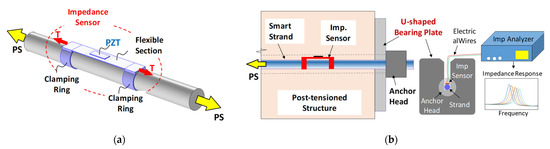
Figure 1.
Overview of the smart strand technique for post-tensioned structures. (a) Smart strand concept; (b) Measurement system.
Figure 1b shows a simple setup for the implementation of the smart strand for a post-tensioned structure. A U-shaped bearing plate is designed to prepare the space for wiring the electrical lines of the piezoelectric transducer, which are connected to an impedance analyzer to record the impedance response. As the strand is prestressed, an axial load T is induced into the impedance device through a clamping mechanism, see Figure 1a. The PS variation will alter the axial load in the impedance device, resulting in a change in its resonant frequencies [28]. Therefore, it is feasible to track the PS change by monitoring the frequency shift of the impedance response [1].
2.2. Electromechanical Impedance Response
In order to record the electromechanical impedance response from the smart strand, a harmonic voltage is applied to the PZT transducer. Under the harmonic electrical excitation, the PZT patch is harmonically deformed under the piezoelectric effect, and this deformation harmonically excites the sensing device (i.e., the flexible section of the impedance device), as illustrated in Figure 2a.
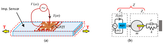
Figure 2.
Illustration of transducer and structure interaction (V(ω): applied voltage, I(ω): current, T: axial load, Za: impedance of PZT, Zs: impedance of host structure, m: mass, c: damping, and k: stiffness constant). (a) Piezoelectric deformation; (b) 1-dof system.
The electromechanical impedance response of the smart strand can be theoretically derived from a 1-dof mass-spring-daspot system, as simplified in Figure 2b [2]. The electromechanical impedance of the smart strand (Z) is a combined function of the mechanical impedance of the piezoelectric transducer (Za) and that of the sensing device (Zs), as follows [29]:
where is the complex Young’s modulus of the piezoelectric transducer (under zero electric field). The parameter is the dielectric constant (zero stress). The term d31 is the coupling constant (under zero stress). The terms wa, la, and ta are the width, length, and thickness of the PZT patch, respectively. The term I is the imaginary unit, and ω is the angular sweep frequency.
The mechanical impedance of the sensing device (Zs(ω)) is defined in the previous reference [29] as follows:
where ωn is the nth natural frequency of the sensing device, which is proportional to the axial load (T) in the impedance device, following the formula [28]:
In Equation (3), Es, Is, ls, ρs, and As are the Young modulus, the inertia moment, the length, the mass density, and the cross-section area of the sensing device (i.e., the flexible section of the impedance device).
On the other hand, the axial load (T) in the sensing device is proportional to the PS load (P), as follows:
in which α is the axial rigidity ratio between the impedance device and the steel strand. ξ is the load transfer factor, representing the amount of the PS load transferred from the strand to the impedance device through the bonded rings. ξ is ranged from 0 to 1. ξ = 1 indicates that the PS load is completely transferred from the strand to the sensing device, while ξ = 0 implies that there is no PS load transfer.
By substituting Equations (2)–(4) into Equation (1) and the resultant electromechanical impedance of the system (Z) can be obtained as [2]:
Equation (5) shows that the electromechanical impedance of the smart strand shall vary with the PS load. Once the sweep frequency matches the natural frequencies of the sensing device, resonant peaks appear in the impedance spectrum, as proved by Equation (2). Therefore, the resonant impedance peaks shift along with the variation of the PS load. The previous studies show that by quantifying those variations, it is feasible to accurately monitor the PS load and estimate the severity of PS change [2,8].
2.3. Potential Faults in Smart Strand
Under working and environmental conditions, the piezoelectric-based smart strand can be damaged, resulting in visible impedance changes, which can be misunderstood as the presence of structural damage (i.e., the PS load change). From the literature [16,21,22,25], we identify four potential fault types that may occur for piezoelectric devices such as the smart strand, including transducer breakage, transducer disbond, shear-lag phenomenon, and device detachment, as illustrated in Figure 3.
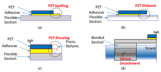
Figure 3.
Illustration of potential failures in the smart strand. (a) Transducer breakage; (b) Transducer disbond; (c) Shear-lag; (d) Device detachment.
Transducer Breakage
It is worth noting that the PZT transducer withstands the operating demands to which its host structure is subjected, such as static/dynamic mechanical loads and environmental influences [18]. The transducer is also subjected to varying electromechanical loading conditions during operation. Those might result in cracking in the PZT patches, as reported in [21] and depicted in Figure 3a. Another possible cause is that during the production process, construction phase, and long-term use, the transducer can be accidentally hit by falling objects, causing damage in terms of crack and/or spalling. The crack and spalling cause reductions in the stiffness of the transducer, leading to changes in its resonant frequencies together with a dropped capacitance. As reported in the literature [25], the transducer spalling can lead to a visible decrease in the slope of the susceptance response.
Transducer Disbond
Debonding at the adhesive region between the transducer and its host structure can lead to a degradation in their electromechanical coupling, as seen in Figure 3b. Insufficient bonding quality and debonding defects might happen right from the beginning due to a contaminated surface during the bonding process, as reported in [30]. While embedded in a post-tensioned structure, the smart strand could be forced to vibrate with the structure under an external load. Such vibrational bendings might also lead to fatigue and disbond of the transducer. The transducer disbond inevitably induces shifts in the electromechanical impedance response. Depending on the disbond severity, either the shift of original resonances or the appearance of additional resonances could occur in the spectrum, as reported in [24,26].
Shear-lag Phenomenon
Shear-lag is the phenomenon when the piezoelectric strain of the PZT is significantly higher than the strain of the host structure under working conditions, as described in Figure 3c [22]. This happens when the thickness of the adhesive layer of the piezoelectric transducer is considerable, or its shear modulus is negligible due to errors during the installation process. After long-term use, the quality of the bonding material may be degraded, causing slippage when the PZT is expanded under an applied voltage. For the smart strand, the shear-lag phenomenon decreases the strain transmission between the transducer and the flexible section of the impedance device and modifies the baseline of the impedance signature, resulting in errors in the PS load estimation.
Device Detachment
Since the impedance device is attached to the smart strand through two bonded rings, it is bent along with the bending of the smart strand. For long-term use under dynamical loads and varying environmental conditions, the attachment capacity of the rings can be degraded, leading to the detachment of the impedance device from the host strand, as illustrated in Figure 3d. It is proved by Equation (4) that the amount of PS load transferred from the strand into the impedance device is proportional to the attachment capacity factor of the bonded rings (ξ). Once the factor ξ alters, the electromechanical impedance spectrum of the smart strand can be shifted. As a result, the estimation of PS load using the impedance spectrum may have significant errors [8]. Thus, the identification of the attachment status of the impedance device is of important interest to secure the performance of the smart strand technique [1].
3. 1D CNN-Based Fault Assessment Method
3.1. Scheme of the Method
Figure 4 illustrates the overall scheme of the 1D CNN-based fault assessment method for the smart strand. The method includes two main phases: (1) data acquisition and (2) training and testing. In the first phase, the raw electromechanical impedance data is collected from the smart strand under different fault types and severities. The collected impedance data is then added by random noises to simulate realistic situations. The original impedance data is used to build the 1D training dataset, while the noise-contaminated impedance data is used to create the 1D testing dataset. In the second phase, a 1D CNN model is established for fault assessment of the smart strand. As sketched in Figure 4, the network is trained by the training dataset, and then its performance is evaluated by the testing dataset.
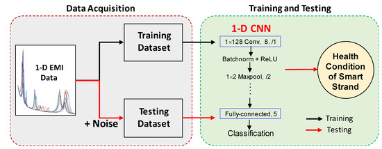
Figure 4.
The 1D CNN-based fault detection method for the smart strand.
Unlike traditional artificial neural networks such as multi-layer perceptron networks, the 1D CNN model can autonomously extract and learn the optimal features from the raw impedance responses (without pre-processing) for damage identification [31,32,33]. As one of the state-of-the-art machine learning models, the 1D CNN algorithm can outperform the conventional neural networks in terms of speed and accuracy, as demonstrated in [31,33,34]. Besides, the network has a simple and compact architecture that does not require high-performance hardware to perform convolutions [35]. Thus, it has the potential to be embedded in real-time impedance-based structural health monitoring systems [33,34,36]. Application of the 1D CNN to process the impedance data has been recently reported. Pioneering researchers made extensive contributions to interface defect classification [20], concrete damage quantification [37], PS load monitoring [38], and assessment of hydration and setting of cement mortar [39]. Nonetheless, the combination of the 1D CNN model and the impedance-based technique for assessing the health condition of the smart strand has not been reported so far.
3.2. 1D CNN-Based Fault Detector
The 1D CNN model is developed to detect and classify the fault types that may occur in the smart strand, as sketched in Figure 5. The architecture of the 1D CNN model is built following the previous well-established models [38,40]. The architecture and hyperparameters of the 1D CNN model were tuned following the practical guidance of Zhang and Wallace [41]. Input of the network has one dimension that fits with the size of the training dataset (i.e., 1D impedance signal with the size of 501 × 1), while the output is the classification of the fault types. As designed, the 1D input layer is sequentially followed by a convolutional layer with 1 × 128 kernel, a maxpooling layer with 1 × 4 kernel, a convolutional layer with 1 × 8 kernel, a maxpooling layer with 1 × 2 kernel, a convolutional layer with 1 × 4 kernel, a fully-connected layer with 128 nodes, a fully-connected layer with 64 nodes, a fully-connected (FC) layer with 5 nodes, a softmax layer, and a classification output layer. Each of those three convolutional layers is followed by a batch normalization layer and a ReLU layer, see Figure 5.
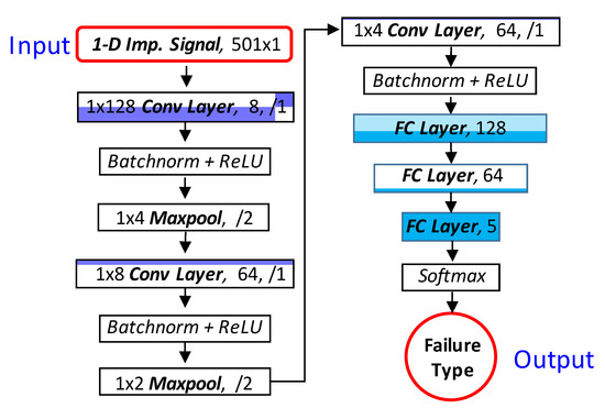
Figure 5.
The block diagram of the 1D CNN model.
The specification of the network’s layers is listed in Table 1, and the principal of the layers are briefly described as follows:

Table 1.
The specification of the layers of the 1D CNN model.
In the convolutional layer, the kernel with weights is designed to learn certain features from the input layer (i.e., the impedance response). The kernel (g) slides over the input data (f) with the strike (s), and the convolution between the kernel and the input layer is calculated (f*g) for each position (i) in the kernel, as follows:
where m is the kernel’s length. As shown in Equation (6), the convolution is accomplished by multiplying the overlapping values of the kernel and the input; the obtained values are then added together; all the results are stacked and output. The output of the convolutional layer is then passed through the ReLU layer to filter the negative values while keeping only positive values. The ReLU layer can help to reduce the computation and training costs. Afterward, the resultant is passed through the batchnorm layer, in which each channel of the input is normalized across a mini-batch to speed up the training process and minimize the sensitivity to the network’s initialization.
In the maxpooling layer, the kernel slides on the input with a strike, and the maximum value is output for each position. This layer helps to reduce the quantity of feature-map coefficients to process and to get spatial-filter hierarchies.
In the FC layer, all nodes are connected to the nodes of the previous layer. For each of the nodes in the FC layer, the dot product is performed on the input. The last fully-connected layer has the number of nodes as the same as the number of classes (i.e., potential fault types).
In the softmax layer, the probability for every possible class is computed using the softmax function [42]. This layer has the same number of nodes as the previous layer (i.e., the fully-connected layer).
In the classification layer, the cross-entropy loss is computed for classification tasks with mutually exclusive classes. The network takes the values from the softmax layer and assigns each input to one of the R mutually exclusive classes using the cross-entropy function for a 1-of-R coding scheme, as follows [42]:
where N is the number of samples, R is the number of classes, wi is the weight for the ith class, tni is the indicator that the nth sample belongs to the ith class, and yni is the probability that the network relates the nth input with the ith class (i.e., the output value from the softmax layer).
4. Finite Element Simulation
Due to the challenges in creating accurate faults in the smart strand via the experiment (such as the shear-lag phenomenon or disbond), this section aims to establish a reliable, verified numerical model that can be used to replace the experiment model for the investigation of electromechanical impedance response of a damaged smart strand. Firstly, the previous experimental test is briefly described. Secondly, a finite element model following the previous experimental structure is established using a commercial program. Finally, the numerical impedance is analyzed, and the simulation result is compared with the experimental data to verify the feasibility of finite element modeling.
4.1. Experimental Test
The impedance response of the smart strand was experimentally recorded in the previous study [2]. The experimental setup is presented in Figure 6. The test structure is a prestressed reinforced concrete girder with a span of 6 m and two overhangs of 0.2 m). A 7-wire smart strand was used for prestressing the girder, as seen in Figure 6. The dimensions and material properties of the smart strand can be found in the reference [8] and detailed in Section 3.2. An impedance device with a length of 70 mm, a width of 10 mm, and a thickness of 0.5 mm was designed and attached to a 7-wires steel tendon to prepare the prestressing smart strand. The tendon has a nominal diameter of 15.2 mm, a nominal area of 138.7 mm2, and an ultimate strength of 1900 N/mm2 [43].
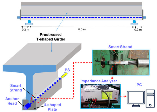
Figure 6.
The test structure and its experimental setup [2].
In the middle section, the impedance device was equipped with a PZT transducer (PZT-5A material, a length of 15 mm, a width of 5 mm, and a thickness of 0.508 mm). A U-shaped bearing plate with 10 mm thickness was also fabricated and inserted into the anchorage to make room for wiring the impedance device. The test structure was placed in a basement room where the temperature was controlled to avoid the influence of temperature change on the piezoelectric and structural properties of the smart strand.
The impedance response was recorded for different PS levels ranging from 1 ton (9.81 kN) to 5 tons (49.05 kN). A stressing jack with 50 tons capacity was used for prestressing the girder through tensioning the smart strand. The applied PS load was measured by a load cell and read by a digital indicator. A commercial impedance recorder, HIOKI 3532, was used to apply a 1V harmonic voltage on the PZT transducer and to measure the electromechanical impedance. The considered frequency band ranged from 0.5 kHz to 10.5 kHz with a 0.02 kHz frequency interval (501 sweep points).
4.2. Finite Element Modelling
The finite element model of a smart strand segment corresponding to the experimental structure was established by the commercial program COMSOL, following the well-established model [7]. We adopted the COMSOL program due to its strong capacity for modeling different complex piezoelectric devices, as demonstrated in the previous studies [44,45,46,47,48]. The solid mechanic module and the electromechanical module available in the COMSOL program were combined to model the piezoelectric effects. The frequency-domain perturbation study was conducted to analyze the electromechanical impedance of the smart strand, considering geometric nonlinearities induced by the PS load. The problem is solved by the framework of the finite-strain theory, in which the strain is represented by the Green–Lagrange strain tensor [49]. The Green–Lagrange strain method is regarded as more accurate than the engineering strain approach [50].
As shown in Figure 7a, the finite element model is a segment of the smart strand (160 mm in length) equipped with an impedance device. The PZT patch (type 5A) is bonded on the top surface of the flexible section of the impedance device via a bonding layer (thickness of 0.1 mm), and the whole piezoelectric device is attached to the strand using two elastic layers (thickness of 0.1 mm). A part of the anchor head is fixed while the PS load is applied to the other end of the strand, as shown in Figure 7a. The geometry of the finite element model follows the actual sizes of the previous experimental structure, as presented in [2] and sketched in Figure 7b. The meshed finite element model is shown in Figure 7c. To mesh the model, we used the user-control meshing type in the COMSOL program with finer meshing for the PZT patch and the impedance device. The meshed model includes 1828 elements (756 prism elements and 1072 hexahedral elements).
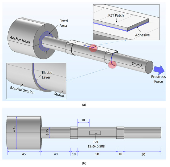
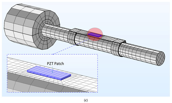
Figure 7.
Finite element modeling of the smart strand. (a) Geometry of the finite element model: 3D view (unit: mm); (b) Geometry of the finite element model: top view (unit: mm); (c) Meshing of the finite element model.
The mechanical properties of the finite element model are shown in Table 2, and the piezoelectric properties of the PZT transducer are listed in Table 3, following the data presented in the reference [7]. The 7-wire strand has a cross-section area of 138.7 mm2 which is smaller than the cross-section area of the simulated strand, 176.7 mm2. Therefore, the mass density and Young’s modulus of the simulated strand were multiplied by a ratio of 0.78. The damping ratio of 0.02 was applied for all structural elements in the whole finite element model, which is consistent with the value presented in [45,51]. The mechanical damping of the PZT patch was simulated using the Rayleigh damping with 0.2 for both frequencies at 0.75 kHz and 8 kHz. In the finite element model, two elastic layers represent the attachment capacity of the impedance device, as shown in Figure 7a. The mechanical properties of the elastic layers are the Poisson’s ratio of 0.38, the mass density of 1700 kg/m3, and the shear modulus of 15 Mpa, those are adopted from the previous study [7].
Table 2.
Mechanical properties of the smart strand [7].
Table 3.
Piezoelectric properties of the transducer [7].
Similar to the previous experiment, a 1V harmonic voltage was assigned to the top of the transducer while the zero potential was applied to the bottom of the transducer. The electromechanical impedance was numerically computed for the frequency from 0.5 kHz to 10.5 kHz (501 sweep points and 0.02 kHz interval). The impedance analysis was conducted for five testing cases, including prestress-loss tests, shear-lag tests, transducer debonding tests, transducer breakage tests, and device detachment tests.
4.3. Feasibility of Finite Element Model
Figure 8 presents the comparison of the results between the simulation and the experiment for the PS level of 5 tons (49.05 kN). Similar to the experiment, the numerical resistance (i.e., the real impedance) shows four resonant peaks, including Resonance 1 in 0.5–1.2 kHz, Resonance 2 in 2–3 kHz, Resonance 3 in 4.5–6.5 kHz, and Resonance 4 in 7.7–9.5 kHz (see Figure 8a). The numerical reactance (i.e., the imaginary impedance) also shows good consistency with the experimental result (see Figure 8b). The frequency of the four resonances was extracted from the simulated impedance response and compared to the experimental data, as shown in Figure 9. It can be observed that the simulated resonant frequencies and the experimental result are well-consistent. Although there exist gaps in the magnitude, the resonances of the resistance and the pattern of the reactance predicted by the finite element model are identical to the previous experiment. Thus, it is feasible to utilize the finite element model for the modeling of potential faults in the smart strand in the following section.
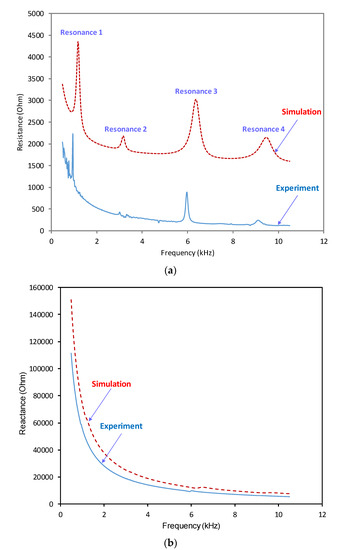
Figure 8.
Electromechanical impedance response of the smart strand: simulation vs. experiment. (a) Real impedance (Resistance); (b) Imaginary impedance (Reactance).

Figure 9.
Resonant frequencies: simulation vs. experiment.
5. Impedance Response of Smart Strand with Faults
The verified finite element model is adopted to study the electromechanical impedance response of the smart strand with faults and PS-loss events. Five simulation sets are run, including the PZT breakage, the PZT debonding, the shear-lag phenomenon, the device detachment, and the PS-loss simulations. Consequently, the effect of the faults and PS-loss on the resistance, the reactance, and the susceptance responses of the smart strand is analyzed to identify the impedance characteristics of the damaged smart strand.
5.1. Transducer Breakage Simulation
In order to model the PZT breakage defect, the length of the PZT transducer in the finite element model was reduced by 20% (breakage 1), 40% (breakage 2), 60% (breakage 3), and 80% (breakage 4). The resistance, the reactance, and the susceptance of the smart strand under the healthy state and four spalling cases of the PZT transducer are shown in Figure 10a–c, respectively. It is observed that the whole resistance curve significantly shifts up according to the amount of transducer spalling, see Figure 10a. While the frequency of the first resonance remains quite stable, that of the third resonance visibly decreases. These observations contradict those observed from the resistance curve in the previous study [24]. It is also noticed that the resonances become less sharp as the spalling size increases. When the spalling severity reaches 80%, the magnitude of the resonances becomes negligible.
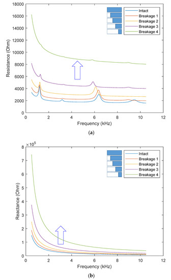
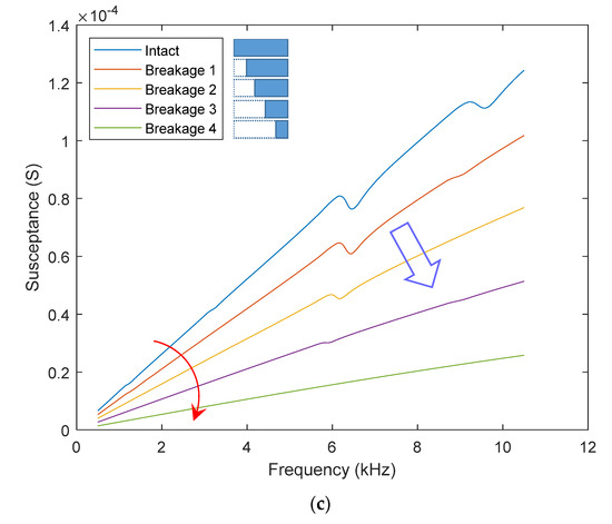
Figure 10.
Impedance response: PZT breakage simulation. (a) Resistance; (b) Reactance; (c) Susceptance.
The reactance curve in Figure 10b exhibits a consistent shift with the previous observation [24]; the curve shifts up when the PZT transducer is broken. As shown in Figure 10c, the slope of the susceptance response, which is known as a good damage indicator [19], significantly decreases with the spalling size of the transducer. This result is well-consistent with the previous study [19].
5.2. Transducer Disbond Simulation
In the finite element model, the length of the bonding layer of the PZT transducer was reduced by 20% (debonding 1), 40% (debonding 2), 60% (debonding 3), and 80% (debonding 4) to simulate the debonding defect. Figure 11a–c, respectively, show the resistance, the reactance, and the susceptance of the smart strand under the healthy state and four debonding cases. As observed from Figure 11a, the resonant peaks in the resistance curve shift down with an increased debonding severity. When the debonding size reaches 80%, the resonant magnitudes become ignorable. The observation on the resistance curve is consistent with those observed in the previous study [24].
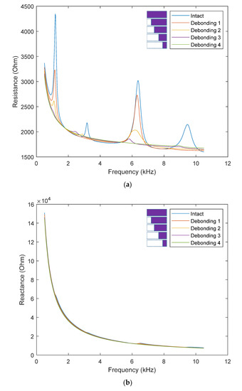
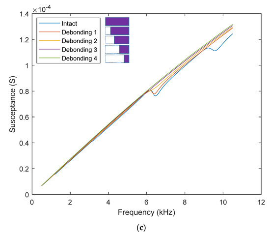
Figure 11.
Impedance response: PZT bebonding simulation. (a) Resistance; (b) Reactance; (c) Susceptance.
However, the reactance curve in Figure 11b shows a contradictory trend with the previous observation. The reactance response of the smart strand remains nearly unchanged despite the disbond of the PZT transducer. Meanwhile, in [19,24], the PZT debonding causes downward shifts in the reactance curve. Although there exist some visible variations in the frequency band of 6–10 kHz, the slope of the susceptance response generally remains stable under the disbond of the PZT transducer (see Figure 11c). This result contradicts the previous observation [19,24], which shows a decreased susceptance slope due to the debonding effect.
5.3. Transducer Shear-Lag Simulation
We modeled the shear-lag phenomenon of the PZT transducer by reducing the shear modulus of the adhesive layer in the finite element model. Ten cases of the reduced shear modulus were simulated with the modulus rate from 0.9 to 0.1 (0.1 steps) and 10−6. The simulated resistance, reactance, and susceptance parts are shown in Figure 12a–c, respectively. The shear-lag phenomenon causes minor changes in the peak frequency, as observed in Figure 12a. Interestingly, some parts of the resistance curve shift down while the other parts shift up. These observations contradict those observed on other piezoelectric devices [24,25]. Although the shear-lag also induces downward shifts in the reactance curve, the shifts are inconsiderable in comparison with the previous observation [24].
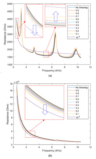
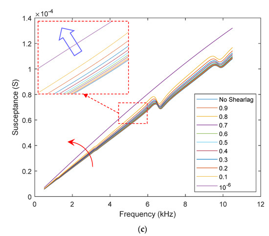
Figure 12.
Impedance response: PZT shear-lag simulation. (a) Resistance; (b) Reactance; (c) Susceptance.
It is known that the mechanical coupling between the PZT transducer and the host structure is dependent on the shear modulus of the bonding layer [52]. When the modulus rate reaches an ignorable value (10−6), no piezoelectric strain is transferred from the PZT to the flexible section, and no contribution of the structural impedance (Zs) is contributed to the overall impedance (Z), according to Equation (1). Therefore, all resonances of the impedance device are disappeared from the resistance curve. As shown in Figure 12c, the susceptance part, which is commonly used to diagnose the PZT transducer, shows an increased slope due to the shear-lag phenomenon. This observation is well-agreed with the previous study [25].
5.4. Device Detachment Simulation
In the finite element model, the detachment of the impedance device is simulated by removing the elastic layer of the bonded rings. Seven cases of device detachment were modeled, as follows: detachment 1 (removing 25% elastic layer of the left ring), detachment 2 (removing 50% elastic layer of the left ring), detachment 3 (removing 75% elastic layer of the left ring), detachment 4 (removing 100% elastic layer of the left ring), detachment 5 (removing 100% elastic layer of the left ring + 25% elastic layer of the right ring), detachment 6 (removing 100% elastic layer of the left ring + 50% elastic layer of the right ring), and detachment 7 (removing 100% elastic layer of the left ring + 75% elastic layer of the right ring).
Figure 13a–c, respectively, show the resistance, reactance, and susceptance responses of the smart strand under the intact state (i.e., healthy case) and detachment 1–7. It is observed that the device detachment causes visible variations in the resonances of the impedance device, see Figure 13a. Several new resonances appear in the resistance curve, generated by the varied boundary condition of the device. For the healthy state, two ends of the flexible section are constrained by the two rings, and the impedance device produces only symmetric modes. If one end is completely/partially released, the impedance device is subjected to new boundary conditions, and thus new resonances with asymmetric modes are created in the frequency spectrum. It is noted that the reactance response remains stable regardless detachment of the impedance device. The device detachment does not modify the slope of the susceptance response despite certain variations in the frequency range of 5.5–10.5 kHz, as depicted in Figure 13c.
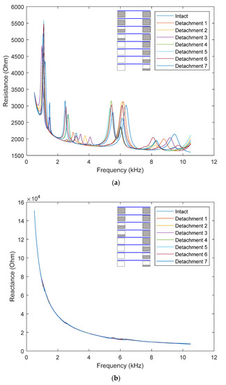
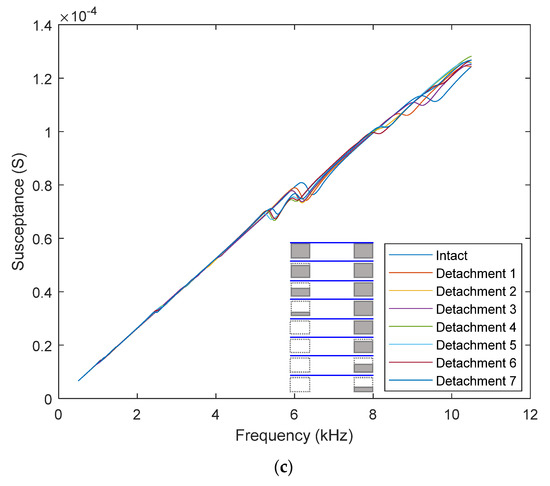
Figure 13.
Impedance response: device detachment simulation. (a) Resistance; (b) Reactance; (c) Susceptance.
5.5. Prestress-Loss Simulation
In order to model the effect of PS-loss on the impedance response, the PS load in the smart strand in the finite element model was gradually reduced from 5 tons (49.050 kN) to 0 kN with an interval of 0.5 tons (4.905 kN). Figure 14a–c, respectively, show the resistance, reactance, and susceptance of the smart strand under the effect of PS-loss. All four resonances in the resistance curve in Figure 14a show visible leftward shifts when the PS load is reduced, suggesting the reduction in the natural frequency following Equation (3). This changing trend is well-agreed with the experimental result [2]. The PS-loss does not modify the reactance curve, as revealed in Figure 14b. Although some visible variations can be observed in the resonant bands, the slope of the susceptance response remains stable regardless of the change in the PS load, as observed in Figure 14c.
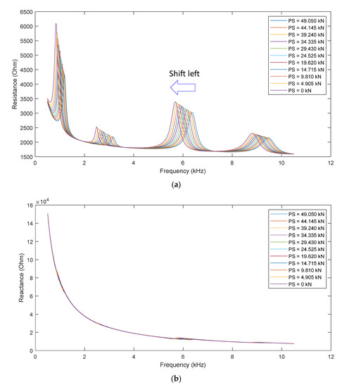
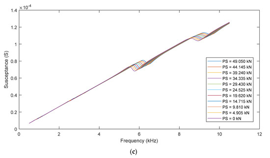
Figure 14.
Impedance response: PS-loss simulation. (a) Resistance; (b) Reactance; (c) Susceptance.
6. Fault Assessment in Smart Strand Using 1D CNN Model
6.1. Databank
In the previous study [20], the reactance response (i.e., the imaginary impedance) was successfully used to assess various functional degradations in a smart interface. The susceptance response (i.e., the imaginary admittance) is also known as a good indicator for diagnosing the PZT defects such as crack and disbond, as reported in [19,24,25]. In the present work, three different response types of the smart strand (i.e., the susceptance response, the reactance response, and the resistance response) are used to construct the databank for the 1-D CNN. From that, the most suitable response for the network is identified.
Three training datasets were built using the data presented in Section 4, including TrainD1 (the resistance dataset), TrainD2 (the reactance dataset), and TrainD3 (the susceptance dataset). Each of the three training datasets has 36 signals, comprising 4 signals for the PZT breakage class (see Figure 10), 4 signals for the PZT disbond class (see Figure 11), 10 signals for the shear-lag class (see Figure 12), 7 signals for the device detachment class (see Figure 13), and 11 signals for the healthy class (1 intact + 10 PS-loss, see Figure 14).
White noises with different levels of 1–8% (1% step) were added to construct the training datasets. This is for the consideration of real measurement conditions in which electrical noises are unavoidable. It is noted that the noise percents are the standard deviations of the signal amplitude. Totally, three corresponding testing datasets TestD1 (the resistance dataset), TestD2 (the reactance dataset), and TestD3 (the susceptance dataset). The sample noise-contaminated resistance signals of the testing dataset (TestD1) are shown in Figure 15. The added white noises cause visible shifts in the resistance curves. Each of the three testing datasets has 288 signals, comprising 32 signals for the PZT breakage class, 32 signals for the PZT disbond class, 80 signals for the shear-lag class, 56 signals for the device detachment class, and 88 signals for the healthy class (8 intact + 80 PS-loss).
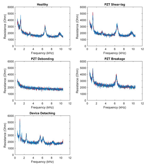
Figure 15.
Sample noise-contaminated resistance signals of the testing dataset (TestD1).
6.2. Training and Testing 1D CNN-Based Fault Detector
A desktop computer (Processor: 11th Gen Intel® Core ™ i7-11700K @ 3.6 GHz (16 CPUs), memory: DDR4 of 32 GB, GPU: NVIDIA GeForce GTX 1660 SUPER of 6 GB) was used to conduct the experiments in this work. We built the 1D CNN model using the MATLAB program. The network was trained using stochastic gradient descent with a momentum algorithm. The training options were set as follows: the mini-batch size of 64, the maxepochs of 400, the initial learning rate of 0.001, the learning rate drop factor of 0.1, the learning rate drop period of 20, and the momentum of 0.9. For every epoch, the training data was shuffled to reduce the overfitting and variance.
Figure 16a shows the training accuracy of the 1D CNN model for different training datasets (TrainD1–TrainD3). The network trained on TrainD1 (the resistance response) yields the highest accuracy (94.4%), while TrainD2 (the reactance response) shows the lowest accuracy (61.1%), and the training accuracy for TrainD3 (the susceptance response) is relatively high (75%). The training loss of the 1D CNN for different training datasets (TrainD1–TrainD3) is shown in Figure 16b. After the 400 iterations, the loss of the network is significantly reduced. The network trained on TrainD1 shows an ignorable loss value (only 0.15) which is the lowest among the three datasets. TrainD2 shows the highest loss at 0.91 while that for TrainD3 is 0.70.
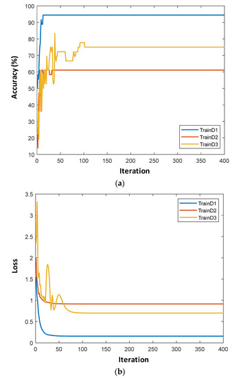
Figure 16.
The training accuracy and the training loss of the 1D CNN. (a) Training accuracy; (b) Training loss.
Next, the performance of the 1D CNN-based fault detector was tested using the noise-contaminated datasets (TestD1–TestD3). The diagnosis results are shown in Figure 17a–c, respectively. In the figures, the predicted classes correspond to the rows of the chart, while the true classes correspond to the columns of the chart. The accurately classified observations correspond to the diagonal cells, while the off-diagonal cells correspond to incorrectly classified observations. The number of observations and the percentage is shown in each cell. In the far-right column of the chart, for each class, the precision (positive predictive value) is presented in green, while the false discovery rate is shown in red. In the bottom row of the chart, for each class, the recall (true positive rate) is shown in green, while the false negative rate is shown in red. The overall accuracy is displayed on the bottom right cell of the chart.
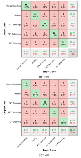
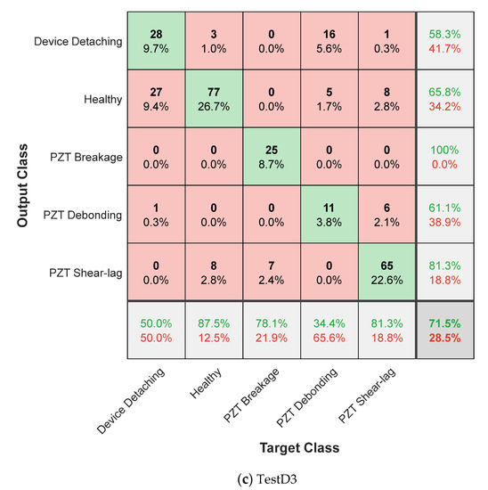
Figure 17.
Testing accuracy of the 1D CNN-based fault detector.
The classification result of TestD1 (the resistant response) is shown in Figure 17a. The predicted classes and the true classes are well-consistent. Despite that, 10% of the shear-lag data was incorrectly classified as the PZT debonding defect, while 9.1% of the health data was incorrectly classified as the shear-lag defect. However, the overall testing accuracy for TestD1 is up 94.1% (see Figure 17a).
The network trained on the dataset TestD2 (the reactance response) continues to show the lowest overall testing accuracy, merely 60.4% (see Figure 17b). Besides, the trained network completely failed to distinguish the device detachment and the PZT debonding from the healthy class. This is due to the nature of the reactance data. As shown in Figure 11b, Figure 13b, and Figure 14b, the reactance response remains almost the same regardless occurrence of the faults.
The testing accuracy of the network trained on the dataset TestD3 (the susceptance response) is presented in Figure 17c. The overall accuracy accounts for 71.5%. Although the accuracy for TestD3 is higher than that for TestD2, the trained network is not able to accurately classify the healthy, the PZT debonding, and the device detachment classes, as observed in Figure 17c.
Figure 18 summarizes the training and testing accuracies of the network trained on the three responses. It is shown that the testing accuracy is slightly lower than the training accuracy. Among the three examined responses, the reactance response is found as the most suitable response for the fault assessment in the smart strand, with superior accuracy compared to other responses.
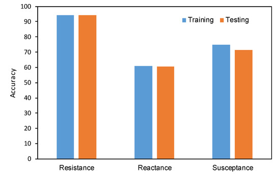
Figure 18.
Comparison of the accuracies of the network trained on three response types of the smart strand.
7. Conclusions
In this study, we analyzed the electromechanical impedance of the smart strand subjected to different fault types using a verified finite element model and proposed a 1D CNN-based fault detector for classifying the potential faults in the smart strand. From the numerical analysis of the impedance characteristics of the smart strand, the following concluding remarks can be drawn from this study:
- The resistance curve of the smart strand significantly shifts up when the transducer is broken. While the frequency of the first resonance remains quite stable, that of the third resonance is visibly decreased. These observations contradict those observed from the resistance curve in the previous study.
- The reactance response and the slope of the susceptance response remain nearly unchanged despite the disbond of the transducer. The result also contradicts the previous observation; that is, the debonding of the transducer causes a downward shift in the reactance curve and a decreased slope of the susceptance response.
- Although the shear-lag defect induces downward shifts in the reactance curve like the previous observation, the reactance shifts are quite ignorable. Interestingly, some parts of the resistance curve shift down while other parts shift up. These observations contradict those observed on other piezoelectric devices.
From the numerical evaluation of the 1D CNN model for assessing the health condition of the smart strand, the key findings are outlined as follows:
- While the susceptance response is widely accepted as a promising feature for detecting faults in piezoelectric devices used in the impedance-based technique, the result from this study shows that the resistance response is more favorable for assessing faults in the smart strand through the 1D CNN method.
- The proposed 1D CNN model, which can automatically extract the optimal features without pre-processing, shows a good performance in classifying the faults of the smart strand. The overall testing accuracy is up to 94.1% when the resistance response is used as the training data.
- The proposed methodology can be integrated with existing impedance-based damage detection systems for real-time structural health monitoring.
Despite the accuracy of finite element modeling, experimental validation is needed to confirm the numerical simulation results. Also, the proposed 1D CNN-based fault detector needs to be validated by the experimental data. Those issues will be addressed in a future study.
Author Contributions
Conceptualization, T.-C.H., D.-D.H., and B.-T.L.; methodology, T.-C.H., D.-D.H., and B.-T.L.; validation, T.-C.H., D.-D.H., B.-T.L., and T.-H.-T.L.; formal analysis, T.-C.H., B.-T.L., T.-C.L., and D.-D.H.; writing—original draft preparation, T.-C.H., B.-T.L., and D.-D.H.; writing—review and editing, T.-C.H. and D.-D.H. All authors have read and agreed to the published version of the manuscript.
Funding
This research received no external funding.
Data Availability Statement
The data are available upon request.
Acknowledgments
We acknowledge Ho Chi Minh City University of Technology (HCMUT), VNU-HCM for supporting this study.
Conflicts of Interest
The authors declare no conflict of interest.
References
- Ryu, J.-Y.; Huynh, T.-C.; Kim, J.-T. Tension force estimation in axially loaded members using wearable piezoelectric interface technique. Sensors 2019, 19, 47. [Google Scholar] [CrossRef] [PubMed]
- Le, T.-C.; Phan, T.T.V.; Nguyen, T.-H.; Ho, D.-D.; Huynh, T.-C. A Low-Cost Prestress Monitoring Method for Post-Tensioned RC Beam Using Piezoelectric-Based Smart Strand. Buildings 2021, 11, 431. [Google Scholar] [CrossRef]
- Park, G.; Sohn, H.; Farrar, C.R.; Inman, D.J. Overview of piezoelectric impedance-based health monitoring and path forward. Shock. Vib. Dig. 2003, 35, 451–464. [Google Scholar] [CrossRef]
- Pham, Q.-Q.; Dang, N.-L.; Kim, J.-T. Smart PZT-Embedded Sensors for Impedance Monitoring in Prestressed Concrete Anchorage. Sensors 2021, 21, 7918. [Google Scholar] [CrossRef]
- Yang, Y.; Liu, H.; Annamdas, V.G.M.; Soh, C.K. Monitoring damage propagation using PZT impedance transducers. Smart Mater. Struct. 2009, 18, 045003. [Google Scholar] [CrossRef]
- Yaowen, Y.; Yee Yan, L.; Chee Kiong, S. Practical issues related to the application of the electromechanical impedance technique in the structural health monitoring of civil structures: II. Numerical verification. Smart Mater. Struct. 2008, 17, 035009. [Google Scholar]
- Nguyen, T.-T.; Ho, D.-D.; Huynh, T.-C. Electromechanical impedance-based prestress force prediction method using resonant frequency shifts and finite element modelling. Dev. Built Environ. 2022, 12, 100089. [Google Scholar] [CrossRef]
- Nguyen, T.-T.; Hoang, N.-D.; Nguyen, T.-H.; Huynh, T.-C. Analytical impedance model for piezoelectric-based smart Strand and its feasibility for prestress force prediction. Struct. Control. Health Monit. 2022, 29, e3061. [Google Scholar] [CrossRef]
- Min, J.; Park, S.; Yun, C.-B.; Song, B. Development of a low-cost multifunctional wireless impedance sensor node. Smart Struct. Syst. 2010, 6, 689–709. [Google Scholar] [CrossRef]
- PPerera, R.; Pérez, A.; García-Diéguez, M.; Zapico-Valle, J.L. Active Wireless System for Structural Health Monitoring Applications. Sensors 2017, 17, 2880. [Google Scholar] [CrossRef]
- Nguyen, K.-D.; Kim, J.-T. Smart PZT-interface for wireless impedance-based prestress-loss monitoring in tendon-anchorage connection. Smart Struct. Syst. 2012, 9, 489–504. [Google Scholar] [CrossRef]
- Park, J.-H.; Kim, J.-T.; Hong, D.-S.; Mascarenas, D.; Lynch, J.P. Autonomous smart sensor nodes for global and local damage detection of prestressed concrete bridges based on accelerations and impedance measurements. Smart Struct. Syst. 2010, 6, 711–730. [Google Scholar] [CrossRef]
- Li, D.; Wang, Y.; Wang, J.; Wang, C.; Duan, Y. Recent advances in sensor fault diagnosis: A review. Sens. Actuators A: Phys. 2020, 309, 111990. [Google Scholar] [CrossRef]
- Zhang, Y.; Wang, X.; Ding, Z.; Du, Y.; Xia, Y. Anomaly detection of sensor faults and extreme events based on support vector data description. Struct. Control. Health Monit. 2022, 29, e3047. [Google Scholar] [CrossRef]
- Worden, K.; Dulieu-Barton, J.M. An Overview of Intelligent Fault Detection in Systems and Structures. Struct. Health Monit. 2004, 3, 85–98. [Google Scholar] [CrossRef]
- Huynh, T.-C.; Nguyen, T.-D.; Ho, D.-D.; Dang, N.-L.; Kim, J.-T. Sensor Fault Diagnosis for Impedance Monitoring Using a Piezoelectric-Based Smart Interface Technique. Sensors 2020, 20, 510. [Google Scholar] [CrossRef]
- Rao, A.R.M.; Kasireddy, V.; Gopalakrishnan, N.; Lakshmi, K. Sensor fault detection in structural health monitoring using null subspace–based approach. J. Intell. Mater. Syst. Struct. 2015, 26, 172–185. [Google Scholar] [CrossRef]
- Taylor, S.; Park, G.; Farinholt, K.; Todd, M. Diagnostics for piezoelectric transducers under cyclic loads deployed for structural health monitoring applications. Smart Mater. Struct. 2013, 22, 025024. [Google Scholar] [CrossRef]
- Park, G.; Farrar, C.R.; Rutherford, A.C.; Robertson, A.N. Piezoelectric active sensor self-diagnostics using electrical admittance measurements. J. Vib. Acoust. 2006, 128, 469–476. [Google Scholar] [CrossRef]
- Nguyen, T.-T.; Kim, J.-T.; Ta, Q.-B.; Ho, D.-D.; Phan, T.T.V.; Huynh, T.-C. Deep learning-based functional assessment of piezoelectric-based smart interface under various degradations. Smart Struct. Syst. Int. J. 2021, 28, 69–87. [Google Scholar]
- Gall, M.; Thielicke, B.; Schmidt, I. Integrity of piezoceramic patch transducers under cyclic loading at different temperatures. Smart Mater. Struct. 2009, 18, 104009. [Google Scholar] [CrossRef]
- Bhalla, S.; Moharana, S. A refined shear lag model for adhesively bonded piezo-impedance transducers. J. Intell. Mater. Syst. Struct. 2012, 24, 33–48. [Google Scholar] [CrossRef]
- Islam, M.M.; Huang, H. Understanding the effects of adhesive layer on the electromechanical impedance (EMI) of bonded piezoelectric wafer transducer. Smart Mater. Struct. 2014, 23, 125037. [Google Scholar] [CrossRef]
- Nguyen, B.-P.; Tran, Q.H.; Nguyen, T.-T.; Pradhan, A.M.S.; Huynh, T.-C. Understanding Impedance Response Characteristics of a Piezoelectric-Based Smart Interface Subjected to Functional Degradations. Complexity 2021, 2021, 5728679. [Google Scholar] [CrossRef]
- Park, S.; Park, G.; Yun, C.-B.; Farrar, C.R. Sensor Self-diagnosis Using a Modified Impedance Model for Active Sensing-based Structural Health Monitoring. Struct. Health Monit. Int. J. 2008, 8, 71–82. [Google Scholar] [CrossRef]
- Mueller, I.; Fritzen, C.-P. Inspection of Piezoceramic Transducers Used for Structural Health Monitoring. Materials 2017, 10, 71. [Google Scholar] [CrossRef]
- Huynh, T.-C.; Kim, J.-T. Impedance-Based Cable Force Monitoring in Tendon-Anchorage Using Portable PZT-Interface Technique. Math. Probl. Eng. 2014, 2014, 11. [Google Scholar] [CrossRef]
- Kim, J.-T.; Yun, C.-B.; Ryu, Y.-S.; Cho, H.-M. Identification of prestress-loss in PSC beams using modal information. Struct. Eng. Mech. 2004, 17, 467–482. [Google Scholar] [CrossRef]
- Liang, C.; Sun, F.P.; Rogers, C.A. Coupled Electro-Mechanical Analysis of Adaptive Material Systems—Determination of the Actuator Power Consumption and System Energy Transfer. J. Intell. Mater. Syst. Struct. 1994, 5, 12–20. [Google Scholar] [CrossRef]
- Mueller, I.; Fritzen, C.-P. Failure Assessment of Piezoelectric Actuators and Sensors for Increased Reliability of SHM Systems. In Structural Health Monitoring from Sensing to Processing; IntechOpen: London, UK, 2018. [Google Scholar] [CrossRef]
- Abdeljaber, O.; Avci, O.; Kiranyaz, M.S.; Boashash, B.; Sodano, H.; Inman, D.J. 1-D CNNs for structural damage detection: Verification on a structural health monitoring benchmark data. Neurocomputing 2018, 275, 1308–1317. [Google Scholar] [CrossRef]
- de Oliveira, M.; Monteiro, A.; Vieira Filho, J. A New Structural Health Monitoring Strategy Based on PZT Sensors and Convolutional Neural Network. Sensors 2018, 18, 2955. [Google Scholar] [CrossRef] [PubMed]
- Ince, T.; Kiranyaz, S.; Eren, L.; Askar, M.; Gabbouj, M. Real-Time Motor Fault Detection by 1-D Convolutional Neural Networks. IEEE Trans. Ind. Electron. 2016, 63, 7067–7075. [Google Scholar] [CrossRef]
- Kiranyaz, S.; Ince, T.; Gabbouj, M. Real-Time Patient-Specific ECG Classification by 1-D Convolutional Neural Networks. IEEE Trans. Biomed. Eng. 2016, 63, 664–675. [Google Scholar] [CrossRef]
- Kiranyaz, S.; Avci, O.; Abdeljaber, O.; Ince, T.; Gabbouj, M.; Inman, D.J. 1D convolutional neural networks and applications: A survey. Mech. Syst. Signal Process. 2021, 151, 107398. [Google Scholar] [CrossRef]
- Zhu, J.; Wang, Y.; Qing, X. A real-time electromechanical impedance-based active monitoring for composite patch bonded repair structure. Compos. Struct. 2019, 212, 513–523. [Google Scholar] [CrossRef]
- Li, H.; Ai, D.; Zhu, H.; Luo, H. Integrated electromechanical impedance technique with convolutional neural network for concrete structural damage quantification under varied temperatures. Mech. Syst. Signal Process. 2021, 152, 107467. [Google Scholar] [CrossRef]
- Nguyen, T.-T.; Tuong Vy Phan, T.; Ho, D.-D.; Man Singh Pradhan, A.; Huynh, T.-C. Deep learning-based autonomous damage-sensitive feature extraction for impedance-based prestress monitoring. Eng. Struct. 2022, 259, 114172. [Google Scholar] [CrossRef]
- Yan, Q.; Liao, X.; Zhang, C.; Zhang, Y.; Luo, S.; Zhang, D. Intelligent monitoring and assessment on early-age hydration and setting of cement mortar through an EMI-integrated neural network. Measurement 2022, 203, 111984. [Google Scholar] [CrossRef]
- Acharya, U.R.; Fujita, H.; Oh, S.L.; Hagiwara, Y.; Tan, J.H.; Adam, M. Application of deep convolutional neural network for automated detection of myocardial infarction using ECG signals. Inf. Sci. 2017, 415-416, 190–198. [Google Scholar] [CrossRef]
- Zhang, Y.; Wallace, B. A Sensitivity Analysis of (and Practitioners’ Guide to) Convolutional Neural Networks for Sentence Classification. arXiv 2015, arXiv:1510.03820b. [Google Scholar]
- Bishop, C.M.; Nasrabadi, N.M. Pattern Recognition and Machine Learning; Springer: Berlin/Heidelberg, Germany, 2006; Volume 4. [Google Scholar]
- Mutalib, A.A.; Mussa, M.H.; Taib, A.M. Behaviour of prestressed box beam strengthened with CFRP under effect of strand snapping. Građevinar 2020, 72, 103–113. [Google Scholar]
- Nguyen, T.-H.; Phan, T.T.V.; Le, T.-C.; Ho, D.-D.; Huynh, T.-C. Numerical Simulation of Single-Point Mount PZT-Interface for Admittance-Based Anchor Force Monitoring. Buildings 2021, 11, 550. [Google Scholar] [CrossRef]
- Huynh, T.-C.; Dang, N.-L.; Kim, J.-T. Preload monitoring in bolted connection using piezoelectric-based smart interface. Sensors 2018, 18, 2766. [Google Scholar] [CrossRef] [PubMed]
- Kitts, D.J.; Zagrai, A.N. Finite Element Modeling and Effect of Electrical/Mechanical Parameters on Electromechanical Impedance Damage Detection. In Proceedings of the ASME 2009 Conference on Smart Materials, Adaptive Structures and Intelligent Systems, Oxnard, CA, USA, 21–23 September 2009; pp. 487–497. [Google Scholar]
- Tashakori, S.; Farhangdoust, S.; Baghalian, A.; Tansel, I.N.; Mehrabi, A. Evaluating the performance of the SuRE method for inspection of bonding using the COMSOL finite element analysis package. In Health Monitoring of Structural and Biological Systems XIII; SPIE: Denver, CO, USA, 2019; pp. 558–568. [Google Scholar]
- Rugina, C.; Enciu, D.; Tudose, M. Numerical and experimental study of circular disc electromechanical impedance spectroscopy signature changes due to structural damage and sensor degradation. Struct. Health Monit. 2015, 14, 663–681. [Google Scholar] [CrossRef]
- Bathe, K.-J. Finite Element Procedures. Prentice Hall: Hoboken, NJ, USA, 2006. [Google Scholar]
- Okereke, M.; Keates, S. Finite Element Applications; Springer International Publishing AG: Cham, Switzerland, 2018. [Google Scholar]
- Cremer, L.; Heckl, M.; Petersson, B.A.T. Damping. In Structure-Borne Sound: Structural Vibrations and Sound Radiation at Audio Frequencies. Springer: Berlin/Heidelberg, Germany, 2005; pp. 149–235. [Google Scholar] [CrossRef]
- Zhou, D.; Ji, T. Free vibration of rectangular plates with continuously distributed spring-mass. Int. J. Solids Struct. 2006, 43, 6502–6520. [Google Scholar] [CrossRef]
Publisher’s Note: MDPI stays neutral with regard to jurisdictional claims in published maps and institutional affiliations. |
© 2022 by the authors. Licensee MDPI, Basel, Switzerland. This article is an open access article distributed under the terms and conditions of the Creative Commons Attribution (CC BY) license (https://creativecommons.org/licenses/by/4.0/).