CFD Simulations of Snowdrifts on a Gable Roof: Impacts of Wind Velocity and Snowfall Intensity

Abstract

Roof structures are suffering serious threats caused by unbalanced snow distribution, especially long-span spatial structures, such as gable roofs. The formation of unbalanced snowdrifts on the gable roof is affected by the meteorological condition and the drifting snow. This study was conducted to explore the snowdrift characteristics on gable roofs under different snowfall conditions based on a new Eulerian–Eulerian multiphase approach. To consider the diffusive process of snow in different states, the governing equations of air and snow phases were modified separately according to the actual transport process. Additional terms based on the deposition/erosion process were inserted into the governing equations to consider the processes of snow particles being trapped or ejected by snow surface. The feasibility of the new model for the snowdrift was validated by comparing with a field observation. Then, the snowdrifts characteristics on typical gable roofs were investigated under different wind velocity and snowfall intensity conditions. The formation mechanism of snowdrifts and the influence of meteorological conditions on snowdrifts were clarified by analysis. The results show that the uneven distribution of snow on the gable roof becomes more significant with the increase in wind velocity. Furthermore, the distribution of snow on the roof tends to be more even in the case of heavier snowfall.

1. Introduction

The frequent occurrence of heavy snowfall has caused many collapse accidents of building structures, resulting in significant economic losses. For example, in 2005, a rare heavy snowfall occurred in Weihai City, Shandong Province, China. The maximum accumulated snow depth reached 80 cm, and 117 houses collapsed. In 2007, Liaoning Province, China, suffered the biggest snowstorm in the past 50 years. The roofs of markets and stadiums in many areas collapsed due to the massive snowfall. In 2008, Southern China was hit by a massive snowstorm which caused millions of houses to collapse or be damaged. In some cases, the maximum depth of snow accumulation on the gable roof was more than 1.5 m. The partial snow load was far beyond the load-carrying capacity of the roofs, resulting in a partial roof collapse, which ultimately led to the overall collapse. According to the statistical results of the accidents, a large amount of gable-roofed buildings collapsed of all the structures. The main reason for such collapse is the partial overload caused by snow drifting and the weak capacity of gable roofs in bearing the unbalanced load. Therefore, the correct prediction of the snow distribution on this kind of roof has great significance in structural design.

The complex interaction of air and snow movement seriously affects the snow loads on roofs. [1]. Therefore, outdoor measurements and wind tunnel experiments were selected to investigate the interaction action first. [2]. Unfortunately, the measurement is greatly affected by the random weather condition, while the experiment is limited by the contradictory similarity numbers [3]. In recent years, computational fluid dynamics (CFD) approaches have been widely used to solve snow-related problems due to their advantages of low cost and high efficiency [4]. Depending on the treatment of the snow phase, the CFD approach could be divided into the Eulerian–Eulerian approach [5,6] or the Eulerian–Lagrange approach [7,8]. Among them, the Eulerian–Eulerian approach is more used in the field of architectural snow engineering because of its low solution requirement [9,10].

For the Eulerian–Eulerian approach, Uematsu et al. [5] took the lead in simulating the snowdrift by introducing an additional scalar equation for falling snow particles and an empirical equation for the near-wall drifting snow particles. This modeling concept was widely used in subsequent numerical simulations of the snowdrift. Okaze et al. [11] proposed a double-equation approach that contained two transport equations of drifting snow density to account for different settling velocities. Tominaga et al. [10] gave a new deposition/erosion model used in the non-equilibrium region where the snowdrift was not fully developed, and the transport equation of drifting snow density was the same as Okaze [11]. Kang et al. [12] used two different transport equations to distinguish saltating and suspended snow particles and conducted a sensitivity analysis of snow cover on flat terrain. Overall, the main problem of these approaches is the lack of consideration of the relative motion between wind and snow, which is not consistent with reality.

Based on these numerical approaches, some researchers attempted to explore snow distributions on roofs in recent years. Zhou et al. [13] simulated the snow load on a flat roof with the consideration of the change in the snow cover. Tominaga et al. [14] investigated the unbalanced snow loads on gable-roofed buildings by considering different wind velocities and roof slopes. More recently, Zhou et al. [15] further explored the snow load characteristics of flat roofs by introducing a snowmelt module into the snowdrift model. Zhou et al. [16] conducted a series of two-dimensional RANS (Reynold-averaged Navier–Stokes) simulations of snow redistribution on a gable roof with various roof slopes. Yu et al. [17] studied snow redistribution on high-low roofs through numerical simulations and experiments. Zhang et al. [18,19] explored the snowdrifts on spherical and arch roofs by using a revised Mixture model. Yin et al. [20,21,22] systematically studied the interference effects of the snow load on building groups with flat or high-low roofs by using experiment and simulation methods. Since most approaches focused on the snow drifting process on even terrain, the simulations of snowdrifts on roofs were carried out by assuming a certain depth of snow cover before introducing wind effects. Actually, the snow drifting phenomenon is more likely to occur during the snowfall even with a low wind velocity. Furthermore, the process of snow drifting is quite different between snowfall and post-snowfall. During the snowfall, complex separation and reattachment would occur when the air flows over the building and changes the movement of snow falling in the air, and drives existing snow drift. The interaction of airflow and snow would cause the redistribution of snow and form a local snowdrift. Therefore, a model that could well reproduce the motion of snow particles in different states is required to investigate the impact of meteorological conditions on snowdrift characteristics.

A Eulerian–Eulerian approach to fully account for the snowfall process is proposed here by considering different particle motion states and the relative motion between air and snow phases. Additional source terms are adopted in the Eulerian–Eulerian approach to consider the processes of snow particles being trapped or ejected by the snow surface. The prediction accuracy of the numerical approach for the snow distribution is validated by the snow distribution around a cube obtained by field observation. Thereafter, a series of CFD simulations are conducted by using the proposed approach to reveal the formation mechanism of snowdrifts on gable roofs and the influence of meteorological conditions.

2. Numerical Approach

2.1. Governing Equations

As the vertical acceleration distance for falling snow particles is much longer than drifting snow particles near the snow surface, the settling velocity of falling snow particles is usually higher than that of drifting snow particles. Therefore, a Eulerian–Eulerian approach is developed in this paper with the consideration of different settling velocities by setting up three phases, namely, the air, falling snow, and drifting snow. The specific equations for different phases are shown below,

$$\frac{\partial {\rho }_{\mathrm{m}}}{\partial t}+\nabla \cdot \left({\rho }_{\mathrm{m}}{\overrightarrow{v}}_{\mathrm{m}}\right)=0,$$

(1)

$$\frac{\partial {\rho }_{\mathrm{m}}{\overrightarrow{v}}_{\mathrm{m}}}{\partial t}+\nabla \cdot \left({\rho }_{\mathrm{m}}{\overrightarrow{v}}_{\mathrm{m}}{\overrightarrow{v}}_{\mathrm{m}}\right)=-\nabla p+\nabla \cdot \left[{\mu }_{\mathrm{m}}\left(\nabla {\overrightarrow{v}}_{\mathrm{m}}+\nabla {{\overrightarrow{v}}_{\mathrm{m}}}^T\right)\right]+{\rho }_{\mathrm{m}}\overrightarrow{g}+\nabla \cdot \left[{\displaystyle \sum _{k=1}^n{\alpha }_k{\rho }_k{\overrightarrow{v}}_{dr,k}{\overrightarrow{v}}_{dr,k}}\right],$$

(2)

where

$${\rho }_{\mathrm{m}}={\displaystyle \sum _{k=1}^n{\alpha }_k{\rho }_k},$$

(3)

$${\overrightarrow{v}}_{\mathrm{m}}=\frac{{\displaystyle \sum _{k=1}^n{\alpha }_k{\rho }_k{\overrightarrow{v}}_k}}{{\rho }_{\mathrm{m}}},$$

(4)

$${\mu }_{\mathrm{m}}={\displaystyle \sum _{k=1}^n{\alpha }_k{\mu }_k},$$

(5)

in which the subscript “m” represents the mixture phase and “k” represents a single phase, such as air, falling snow and drifting snow, respectively. ${\rho }_{\mathrm{m}}$ is the mixture density; ${\overrightarrow{v}}_{\mathrm{m}}$ is the mass weighted mean velocity of mixture phase; ${\mu }_{\mathrm{m}}$ is the viscosity of the mixture phase; ${\alpha }_k$, ${\rho }_k$, ${\overrightarrow{v}}_k$, ${\overrightarrow{v}}_{dr,k}$, ${\mu }_k$ represent the volume fraction, density, velocity, drift velocity, and viscosity of a single phase k, respectively. p represents the pressure; $\overrightarrow{g}$ represents the acceleration of gravity.

The volume fractions of ${\alpha }_{\mathrm{sky}}$ and ${\alpha }_{\mathrm{surf}}$ are obtained by solving the continuous equations of the falling and drifting snow, respectively, as indicated in Equations (6) and (7). The relative motion between air and snow is considered by solving the momentum equation of snow particles, as indicated in Equation (8).

$$\frac{\partial {\alpha }_{\mathrm{sky}}{\rho }_{\mathrm{s}}}{\partial t}+\nabla \cdot \left({\alpha }_{\mathrm{sky}}{\rho }_{\mathrm{s}}{\overrightarrow{v}}_{\mathrm{m}}\right)=-\nabla \cdot \left[{\alpha }_{\mathrm{sky}}{\rho }_{\mathrm{s}}{\overrightarrow{v}}_{\mathrm{dr},\mathrm{sky}}\right],$$

(6)

$$\frac{\partial {\alpha }_{\mathrm{surf}}{\rho }_{\mathrm{s}}}{\partial t}+\nabla \cdot \left({\alpha }_{\mathrm{surf}}{\rho }_{\mathrm{s}}{\overrightarrow{v}}_{\mathrm{m}}\right)=-\nabla \cdot \left[{\alpha }_{\mathrm{surf}}{\rho }_{\mathrm{s}}{\overrightarrow{v}}_{\mathrm{dr},\mathrm{surf}}\right],$$

(7)

$${\overrightarrow{v}}_{\mathrm{dr},\mathrm{sky}}={\overrightarrow{v}}_{\mathrm{dr},\mathrm{surf}}=\frac{{\tau }_{\mathrm{s}}}{f_{\mathrm{drag}}}\frac{\left({\rho }_{\mathrm{s}}-{\rho }_{\mathrm{m}}\right)}{{\rho }_{\mathrm{s}}}\left[\overrightarrow{g}-\left({\overrightarrow{v}}_{\mathrm{m}}\cdot \nabla \right){\overrightarrow{v}}_{\mathrm{m}}-\frac{\partial {\overrightarrow{v}}_{\mathrm{m}}}{t}\right]-{\displaystyle \sum _{k=1}^n\frac{{\alpha }_k{\rho }_k}{{\rho }_{\mathrm{m}}}}\left({\overrightarrow{v}}_{\mathrm{a}}-{\overrightarrow{v}}_k\right),$$

(8)

$${\tau }_{\mathrm{s}}=\frac{{\rho }_{\mathrm{s}}{d}_{\mathrm{s}}^2}{18{\mu }_{\mathrm{a}}},$$

(9)

$$f_{\mathrm{drag}}=\{\begin{array}{cc}1+0.15{\mathrm{Re}}^{0.687}\hfill & , \mathrm{Re}\le 1000\hfill \\ 0.0183\mathrm{Re}\hfill & , \mathrm{Re}>1000\hfill \end{array}.$$

(10)

In Equations (6)–(10), ${\overrightarrow{v}}_{\mathrm{dr},\mathrm{sky}}$ and ${\overrightarrow{v}}_{\mathrm{dr},\mathrm{surf}}$ represent the drift velocity of falling snow and drifting snow, respectively; ${\rho }_{\mathrm{s}}$ represents the pure density of snow particles; ${\overrightarrow{v}}_{\mathrm{a}}$ denotes the air velocity; ${\tau }_{\mathrm{s}}$ denotes the particle relaxation time; f_drag denotes the drag function; d_s denotes the diameter of snow particles; ${\mu }_{\mathrm{s}}$ denotes the snow viscosity. Re denotes the Reynold number.

At the snow surface, complex mass transfer occurs due to erosion and deposition, which leads to the change in snow fraction in the computational domain. To express the processes of snow particles being trapped or ejected by the snow surface, additional terms are inserted into the continuous equations of falling snow (Equation (6)) and drifting snow (Equation (7)), respectively. The modified continuous equations are given as Equations (11) and (12).

$$\frac{\partial {\alpha }_{\mathrm{sky}}{\rho }_{\mathrm{s}}}{\partial t}+\nabla \cdot \left({\alpha }_{\mathrm{sky}}{\rho }_{\mathrm{s}}{\overrightarrow{v}}_{\mathrm{m}}\right)=-\nabla \cdot \left[{\alpha }_{\mathrm{sky}}{\rho }_{\mathrm{s}}{\overrightarrow{v}}_{\mathrm{dr},\mathrm{sky}}\right]+S_{\mathrm{sky}},$$

(11)

$$\frac{\partial {\alpha }_{\mathrm{surf}}{\rho }_{\mathrm{s}}}{\partial t}+\nabla \cdot \left({\alpha }_{\mathrm{surf}}{\rho }_{\mathrm{s}}{\overrightarrow{v}}_{\mathrm{m}}\right)=-\nabla \cdot \left[{\alpha }_{\mathrm{surf}}{\rho }_{\mathrm{s}}{\overrightarrow{v}}_{\mathrm{dr},\mathrm{surf}}\right]+S_{\mathrm{surf}},$$

(12)

where $S_{\mathrm{sky}}$ and $S_{\mathrm{surf}}$ are additional terms that are inserted into the transport equations. Here, two assumptions are made while setting source terms, according to Okaze et al. [11]. The first assumption is that the falling snow is captured immediately once it hits the snow surface. This assumption would lead to a reduction of snow volume fraction in the near-wall region (the nearest cells adjacent to the snow surface). The second assumption is that the eroded snow jumping up from the ground would cause an increase in snow concentration in the surrounding areas. The specific equations of $S_{\mathrm{sky}}$ and $S_{\mathrm{surf}}$ are given by Equations (13) and (14).

$$S_{\mathrm{sky}}=-\frac{q_{\text{sky-dep}}}{h_{\mathrm{sal}}},$$

(13)

$$S_{\mathrm{surf}}=-\frac{q_{\text{sky-dep}}+q_{\mathrm{ero}}}{h_{\mathrm{sal}}},$$

(14)

where $q_{\text{sky-dep}}$ and $q_{\text{surf-dep}}$ represent the deposition flux of two types of snow phases, namely, falling and drifting snow. $q_{\mathrm{ero}}$ is the erosion flux of the snow phase; $h_{\mathrm{sal}}$ denotes the height of the saltation. It needs to be pointed out that deposition and erosion of the snow phase play a direct role in the change in snow concentration within the saltation layer, and the change in snow concentration in the suspension layer is caused by diffusion.

2.2. Erosion and Deposition Model

During a snowfall, the flow field around the building is not fully developed due to the disturbance of the building’s shape. To consider the non-equilibrium snow drifting process, the erosion and deposition models used by Tominaga et al. [10] are selected and modified for different snow phases. The revised equations are listed as follows (Equations (15)–(18)).

$$q_{\text{sky-dep}}=-{\alpha }_{\mathrm{sky}}{\rho }_{\mathrm{s}}{u}_{\mathrm{z}},$$

(15)

$$q_{\text{surf-dep}}=-{\alpha }_{\mathrm{surf}}{\rho }_{\mathrm{s}}{w}_{\mathrm{f}},$$

(16)

$$q_{\mathrm{ero}}=-c_{\mathrm{a}}{\rho }_{\mathrm{s}}{u}_{*}\left(1-\frac{u_{*\mathrm{t}}^2}{u_{*}^2}\right),$$

(17)

$$q_{\mathrm{total}}=q_{\text{sky-dep}}+q_{\text{surf-dep}}+q_{\mathrm{ero}},$$

(18)

where, $u_{\mathrm{z}}$ is the vertical velocity of falling snow; $w_{\mathrm{f}}$ is the settling velocity of drifting snow; $u_{*}$ is the friction velocity; $c_{\mathrm{a}}$ is a constant of 5.0 × 10⁻⁴ [10], which is related to the number of eroded snow particles; $u_{*\mathrm{t}}$ is the threshold friction velocity; $q_{\mathrm{total}}$ is the total deposition flux of the snow phase.

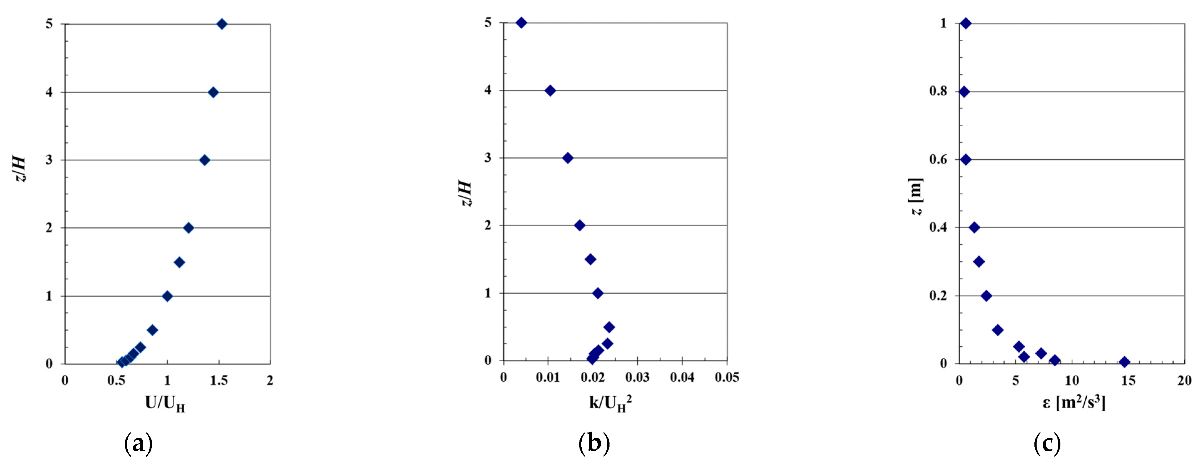
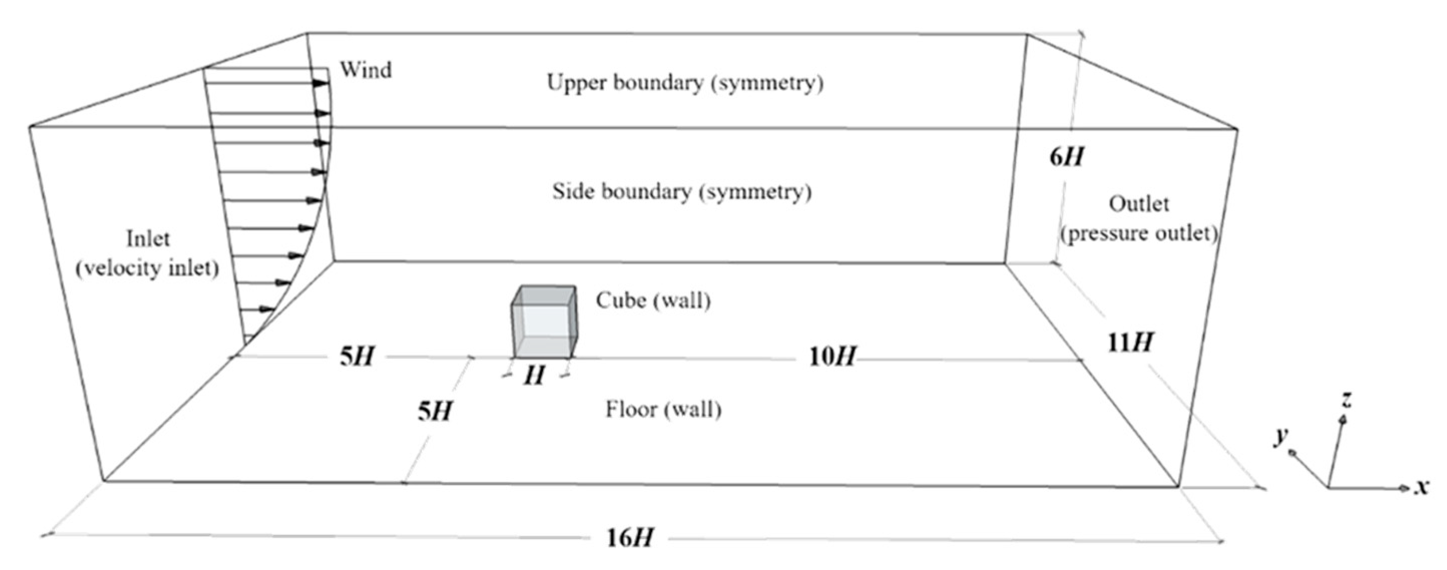
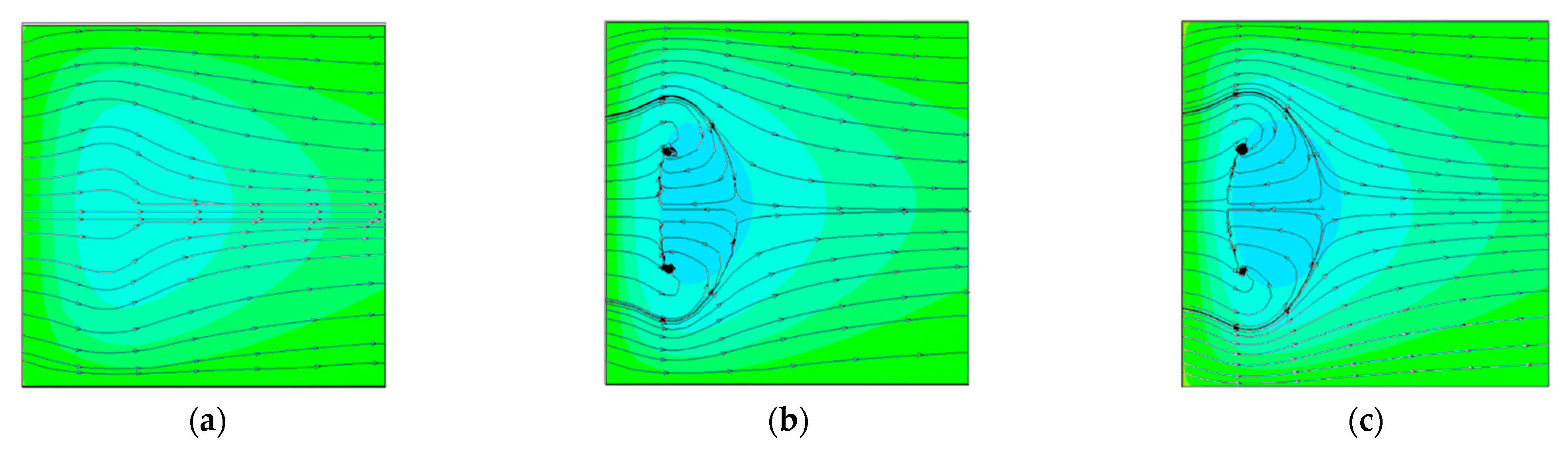
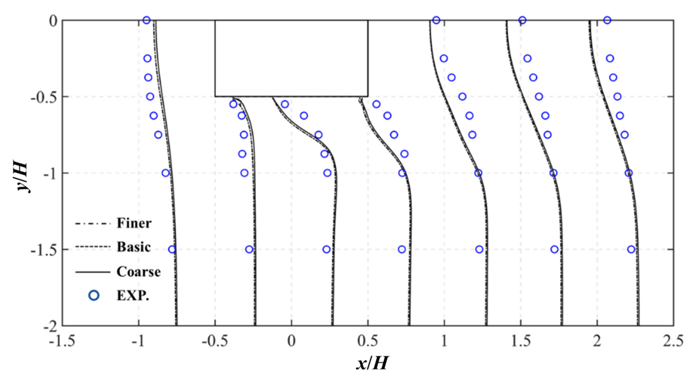
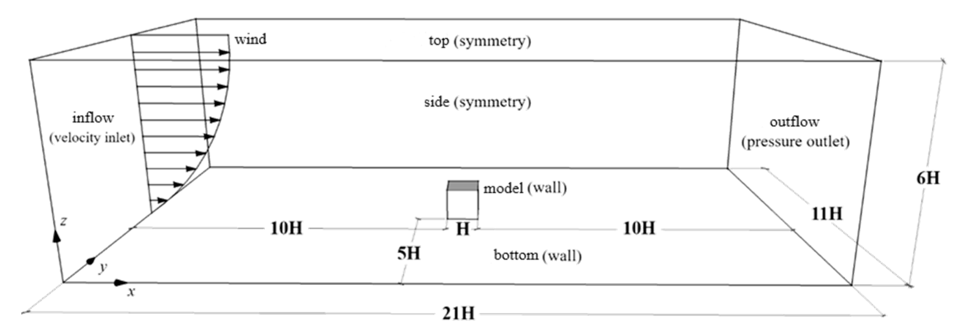
3. Validation of Flow Field

3.1. Prototype of Flow Field

As the air is generally treated as the primary phase that dominates the snow-blowing phenomena, the reproduction of the flow field around buildings becomes quite important to the precise prediction of snowdrifts. Therefore, the predicting accuracy of the flow field was examined first here. The flow field adopted as a test case was around a cubic building model [23]. The side length of the cubic building model H was 0.2 m and the inflow mean velocity at the eave height was about 7.0 m/s. The inflow Reynolds number at the eave height was 9.2 × 10⁴. Figure 1 shows the incident profiles of the flow field.

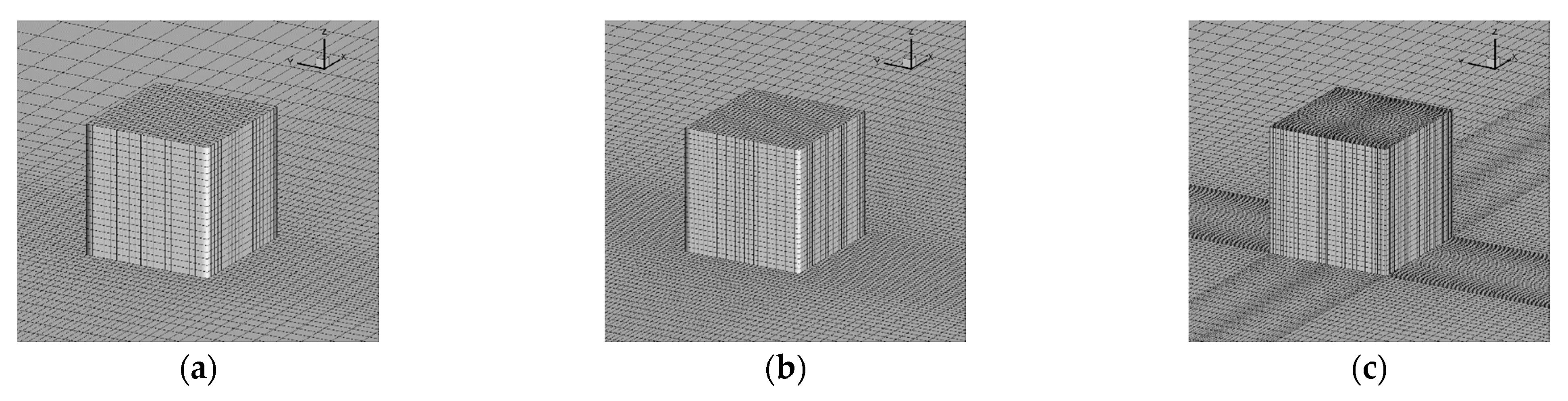
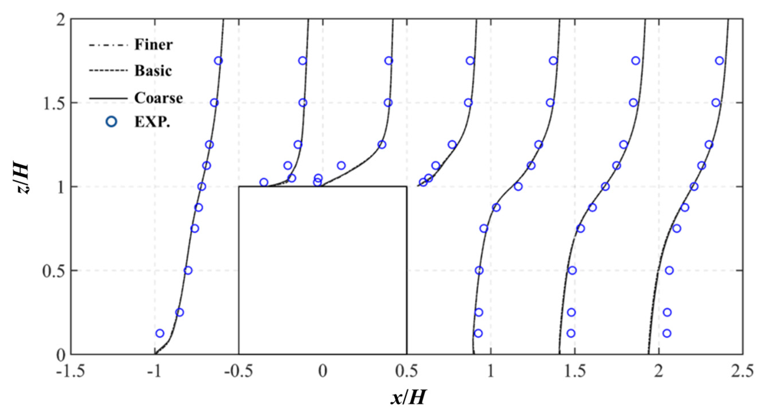
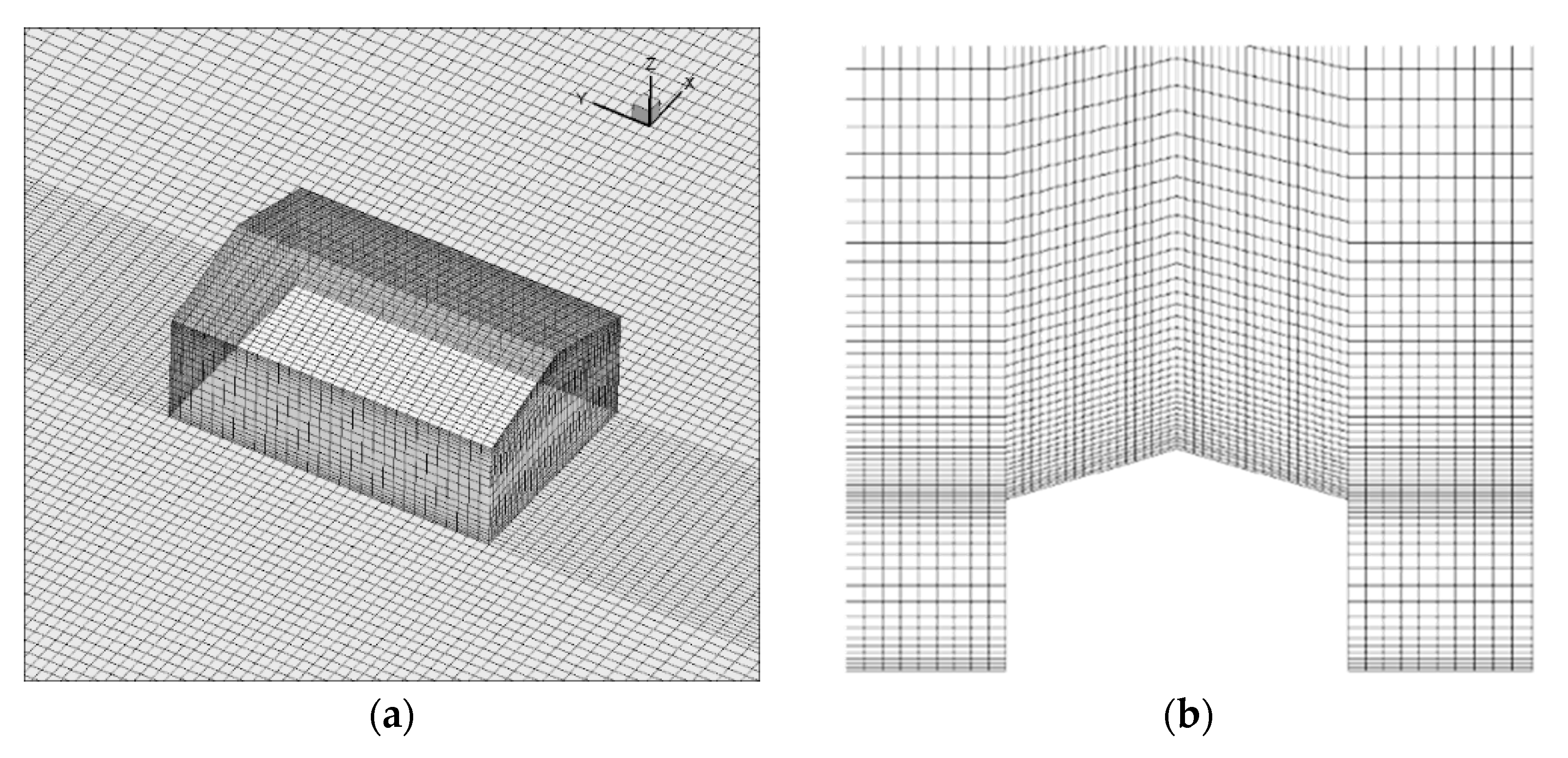
3.2. Computational Details

The settings of the simulation domain are summarized in Figure 2. The domain is 16 H long, 11 H wide, and 6 H high. Three meshing projects with different resolutions were drawn, as shown in Figure 3.

The vertical profiles of the inflow, i.e., the streamwise velocity, the turbulent kinetic energy, and the turbulent dissipation rate, were given according to the experimental results. The vertical velocity profile followed a power law with the power law exponent α = 0.23. The turbulent kinetic energy was calculated based on the velocity and turbulent intensity. For the ground surface, the standard wall function was adopted. The realizable k-ε model was selected to simulate the turbulent structure. The advection terms were discretized using a second-order upwind scheme. The semi-implicit method for the pressure-linked equation (SIMPLE) algorithm was used for the pressure–velocity coupling. The Green–Gauss cell-based scheme was used for gradient discretization. The RMS residual equaling to 10⁻⁷ was taken as the convergence criterion.

3.3. Results and Discussion

Figure 4 gives a comparison of the streamwise velocity for the three meshes at the center vertical section. No deviation is found among the three meshes except for the lower part of the line at x/H = −0.5, however, the deviation is quite small. Figure 5 shows the streamlines at the top of the cube for the three meshes. For the coarse mesh, no reverse flow is reproduced on the building roof, while the reverse flows occur on the two other meshes at x/H ≈ −0.25. Figure 6 gives a comparison of the streamwise velocity at a horizontal section z/H = 0.15. For all the lines, no difference is observed between the basic and finer meshes, however, the streamwise velocity is overestimated by the coarse mesh. Relatively, the basic mesh-based realizable k-ε model could well reproduce the flow field.

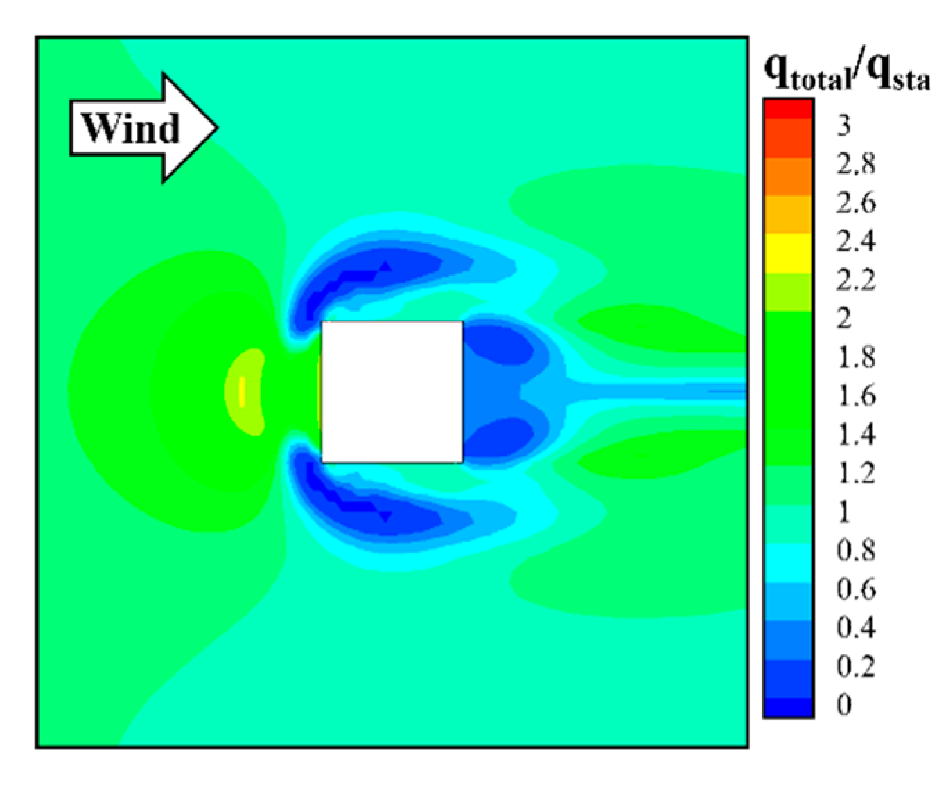
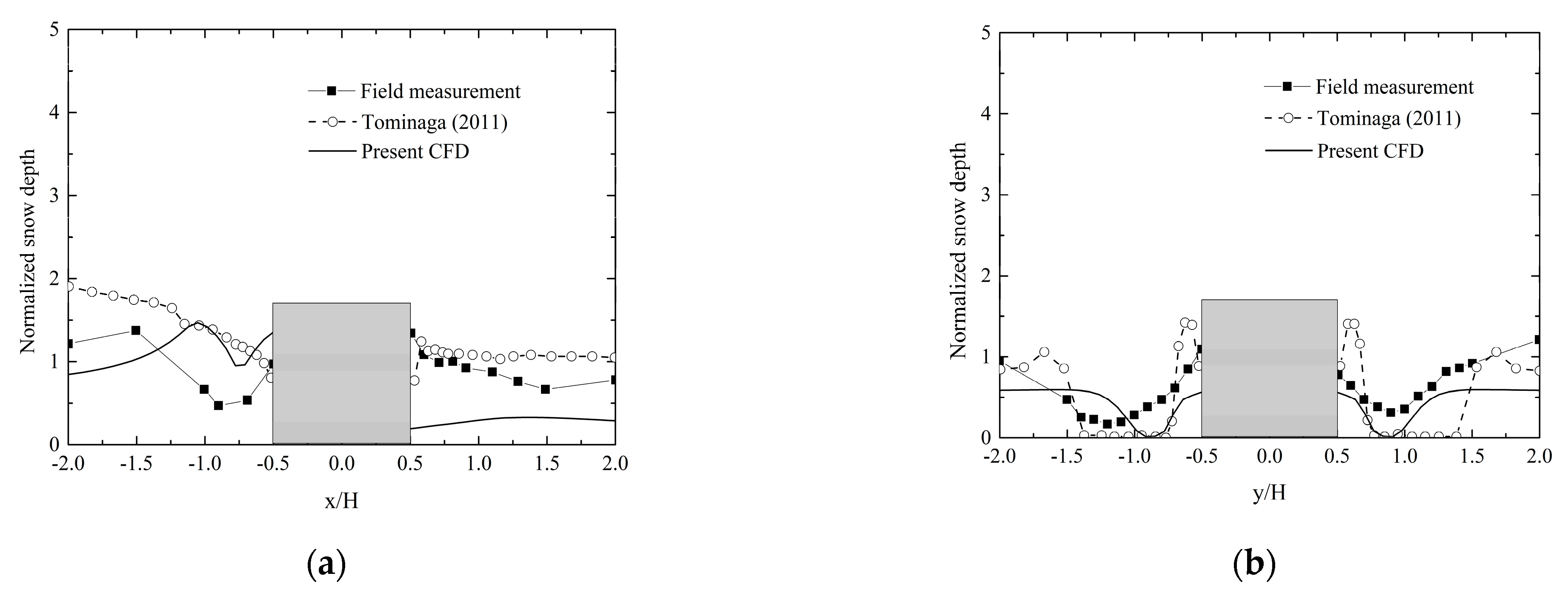
4. Validation of Snowdrift Model

4.1. Prototype of Numerical Simulation

To test the proposed snowdrift approach, a field measurement [24] of the snowdrift around a cubic model (1.0 m long side) was adopted as the comparison prototype. The same measurement data were also used to validate the accuracy of the snowdrift approach in a previous study [10]. The field measurement was conducted in 1998 in Sapporo, Japan by Oikawa et al. [24]. The observation duration of each run was one day removing the remaining snow on and around the model for the next set of measurements.

4.2. Computational Conditions

The computational domain size and boundary conditions settings are shown in Figure 7. The specific size of the computational domain is 21H(x) × 11H(y) × 6H(z), where H represents the length of the model (1.0 m). As the air–snow mixed flow ahead of the model has been fully developed in practice, the fetch distance between the model and the inlet boundary was extended to 10 H (10 m) to ensure the full development of drifting snow. The fetch distance was given to refer to the experimental study on the development process of drifting snow carried out by Okaze et al. [25]. Structural meshes were adopted, and the number of cells in each direction was 200(x) × 120(y) × 70(z). The height of the first cell layer on the bottom boundary was 0.1 m, which approximately equaled to the height of the saltation layer [24].

As there was a long period of weak wind (1~2 m/s) before and after the observation, during which the wall shear stress could hardly reach the critical value at which the snow drifting would occur; therefore, only a gale period with the wind velocity greater than 2 m/s was selected for the snowdrift simulation. During this period, the averaged and median wind velocities were about 2.7 m/s and 2.5 m/s, respectively. Therefore, the simulation inflow velocity was set at 2.5 m/s. The specific inflow boundary conditions are shown in

Table 1. Boundary conditions.

Inflow velocities and turbulence of air and snow phases	$\mathrm{Downwind} \mathrm{velocity}: U=U_{\mathrm{H}}{\left(\frac{z}{H}\right)}^{0.25}$$, U_{\mathrm{H}}$ represents the velocity at height of building eave, which was set at 2.5 m/s.
	The turbulent energy and dissipation rate were given by referring to the papers [10,26].
Inflow snow concentration of different snow phases	0.4 kg/m3 for the saltation layer (z ≤ 0.1 m) for drifting snow [10]. 0.05 kg/m3 for the suspension layer (z > 0.1 m) for falling snow [10].

. The turbulence model, schemes and convergence criterion were set the same as above. The bulk snow density was 150 kg/m³ [10]; the diameter of snow particles was 0.00015 m [10]; the threshold friction velocity was 0.15 m/s [10]; the settling velocity in the saltation layer was 0.2 m/s.

4.3. Results and Discussion

To clarify the formation mechanism of snowdrifts, the horizontal distributions of normalized deposition flux caused by falling and drifting snow, as well as the erosion flux caused by aerodynamic shear stress are discussed first. The flux is normalized by the total deposition flux $q_{\mathrm{sta}}$ at which the snow distribution is unaffected by the cube. Figure 8a,b shows the normalized deposition flux of drifting and falling snow, respectively. Figure 8c illustrates the erosion flux. The deposition of drifting snow is the main part of the total deposition. Saltating particles near the surface are mainly deposited in the surrounding areas away from the cube, while the falling particles are mainly concentrated in the vicinity of the cube. Erosion mainly occurs in the lateral areas where the airflow separates, and the eroded particles are deposited outside the separation flow. The formation of the deposition area at the junction of the windward surface of the cube and the ground is the deposition of falling snow. It should be noted that the snow accumulation at the leeward side of the cube is less than those in other directions. This is partly caused by the blocking effect of the cube, since it is difficult to bring the particles into the wake region.

The total deposition flux can be obtained by summing up the deposition flux of two types of snow phases and the erosion flux. The normalized total deposition flux is shown in Figure 9. Regarding the integral distribution characteristics, deposition is mainly formed in front of the model. The erosion area is formed in the separation area because of the high-speed flow. Quantitative comparisons between numerical analysis results and the field measurement data are given in Figure 10. At the windward side of the streamwise direction, the trend of predicted snow depth is consistent with field measurement. Both the present CFD and field measurement shows two peak values in front of the cube which is not predicted by Tominaga et al. [10]. The present CFD model underestimates the value of normalized snow depth behind the cube. It is mainly because the wind direction fluctuation is not considered in the current numerical simulation and the drifting snow cannot get into the wake region. At the lateral direction, the normalized snow depth of present CFD is in better agreement with the field observation. Generally, the numerical simulation method proposed in this paper is acceptable.

5. Snow Distribution on an Isolated Gable Roof

5.1. Outline of Computations

Due to the characteristic of the lightweight roof, light-steel gable-roofed buildings are very sensitive to snow loads, which leads to a great deal of building collapse accidents. As the snowdrift characteristics have a close relationship with the meteorological condition, snow distributions on the gable roof are investigated firstly by considering different wind velocities and snowfall intensities.

A gable roof with a slope of 3:10 was selected, as similar slopes were widely used in industrial plants. The size of the gable-roofed building was 10 m (x) × 15 m (y) × 5 m (z: eave height), and the computational domain was 130 m long, 60 m wide, and 40 m high. Structural grids were adopted to mesh the computational domain. The total number of cells was about 2.2 million. The height of the near-wall cell was set equal to 0.01 m (y⁺ ranged from 80 to 270) to simulate the saltation layer. Figure 11 shows the cells in detail.

The turbulence model, schemes, and convergence criterion were set the same as above. The parameters of snow particles adopted in this paper are consistent with Zhang et al. [18,19], which are obtained by measured statistics of snow particles. The density of snow particles, diameter, threshold friction velocity, and settling velocity of saltating particles was set to 250 kg/m³, 0.0005 m, 0.2 m/s, and 0.2 m/s, respectively.

It needs to be pointed out that the simulation was conducted without prior snow cover on the roof, which meant the snowfall and snow drifting occurred simultaneously. Therefore, a restriction should be added to the additional term S_surf to ensure that the amount of eroded snow was less than the amount of falling snow captured by snow surfaces, as shown in Equations (19) and (20).

$$S_{\mathrm{surf}}=-\frac{q_{\text{surf-dep}}+q_{\mathrm{ero}}}{h_{\mathrm{sal}}}\hspace{1em}{S}_{\mathrm{surf}}\le -S_{\mathrm{sky}},$$

(19)

$$S_{\mathrm{surf}}=-S_{\mathrm{sky}}\hspace{1em}{S}_{\mathrm{surf}}>-S_{\mathrm{sky}}.$$

(20)

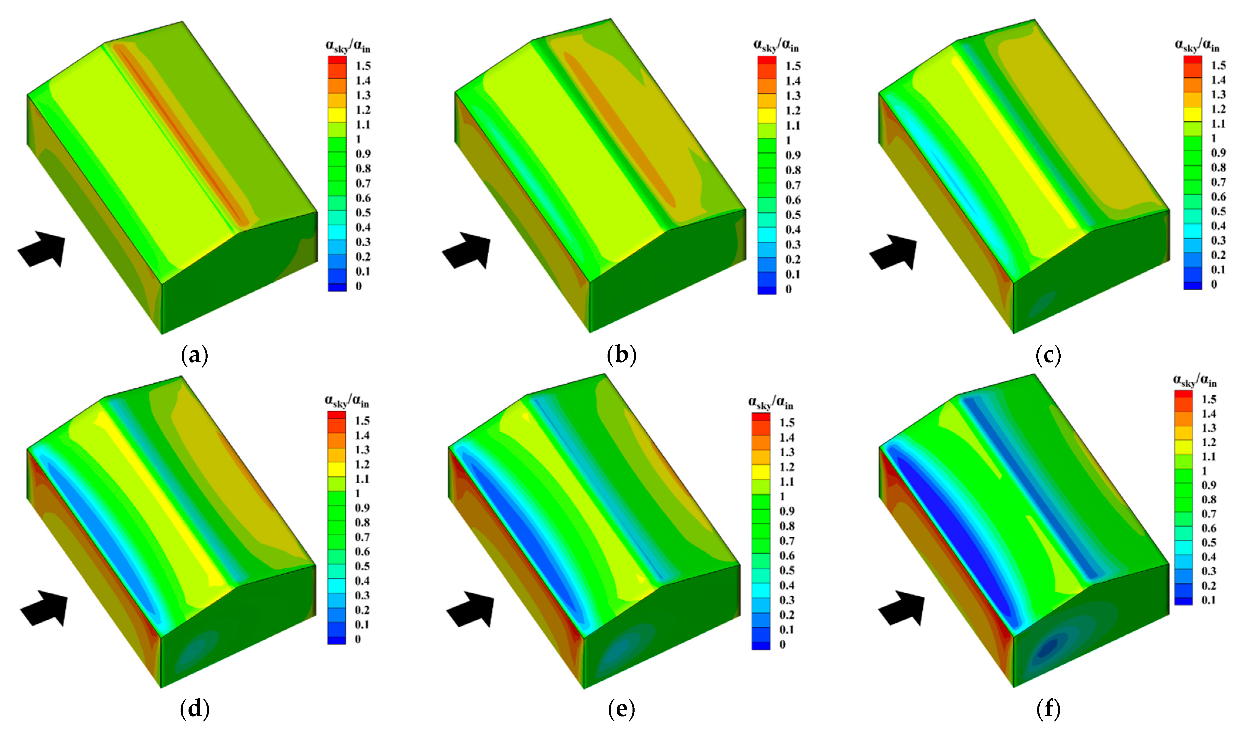
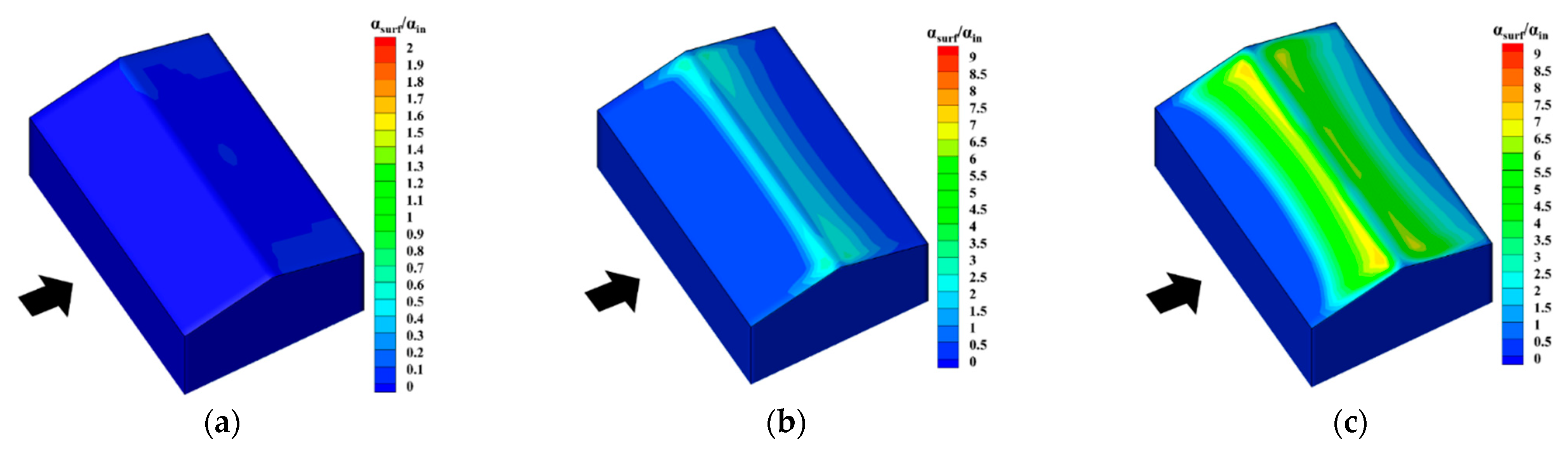
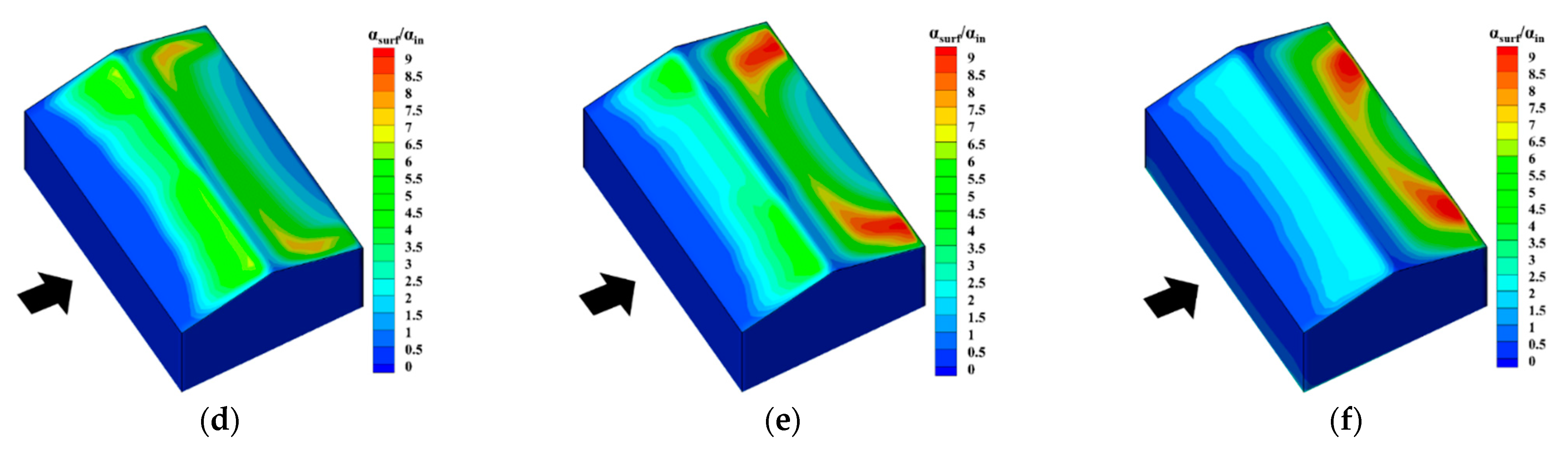
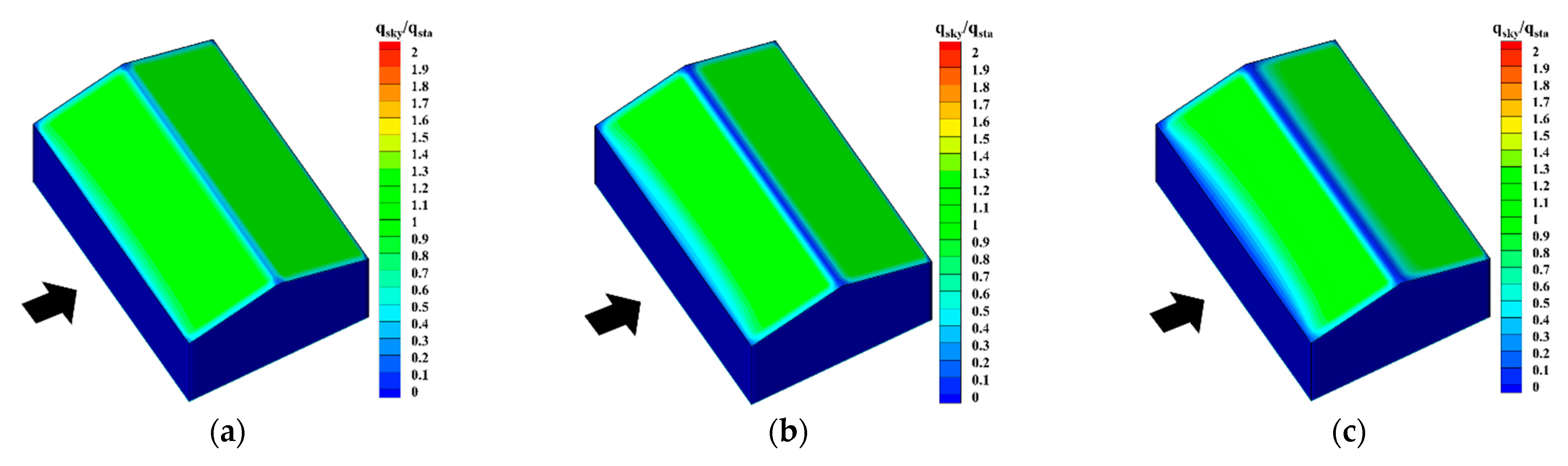
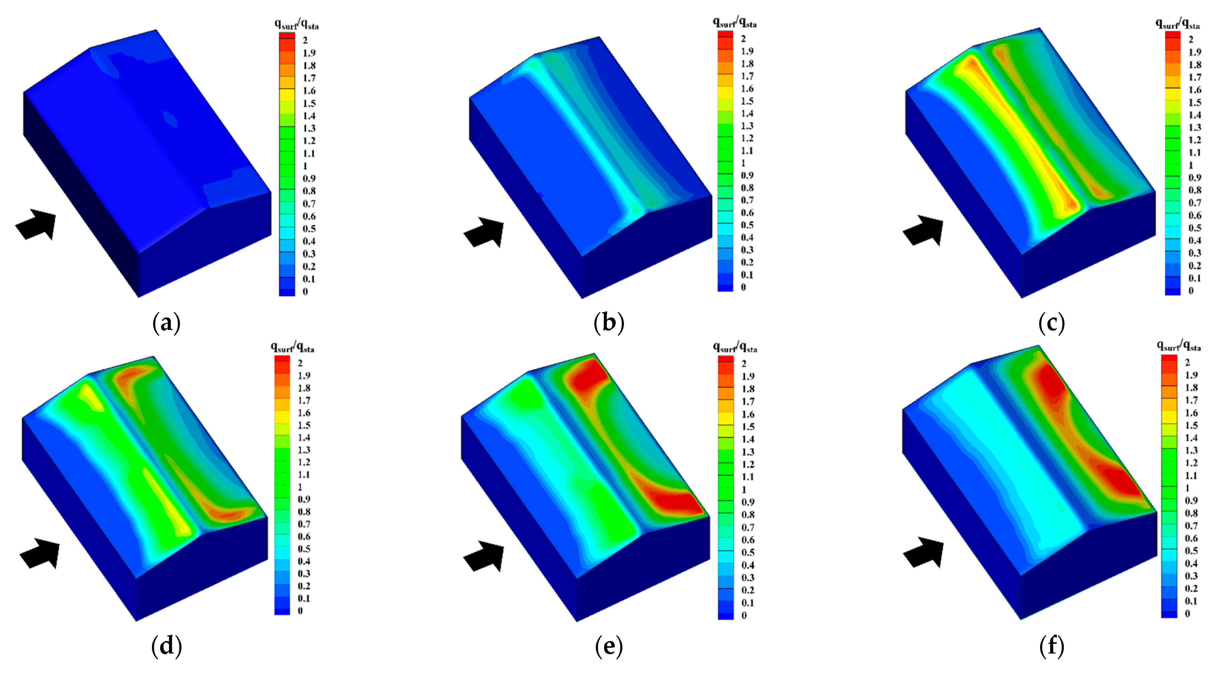
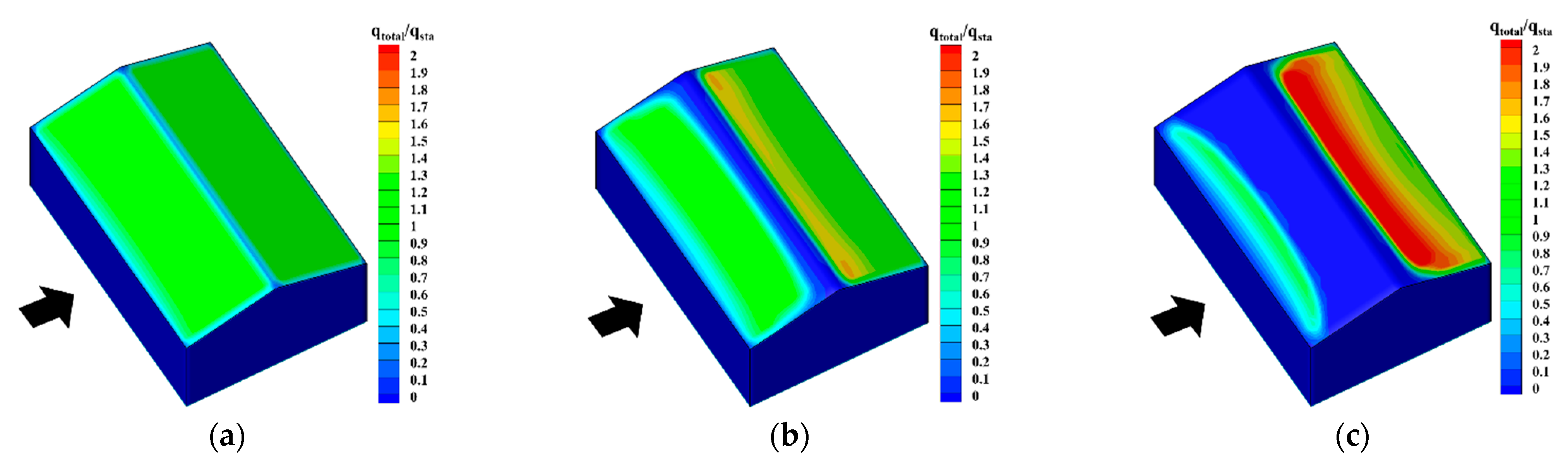
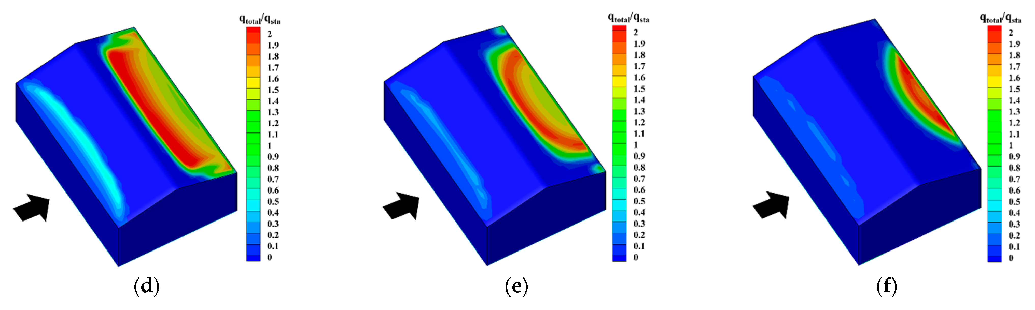
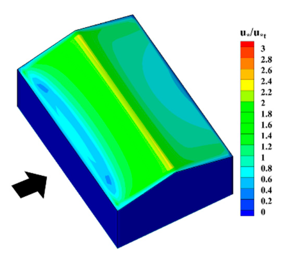
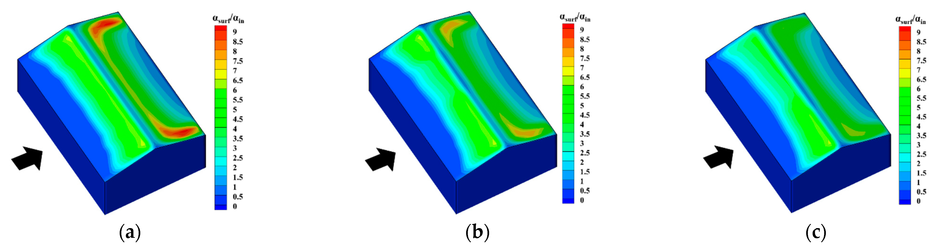
5.2. Impact of Wind Velocity

The snowdrift pattern is closely related to wind velocity. According to the AIJ Recommendations for Loads on Buildings [27], the variation of roof snow only occurs when the wind velocity is greater than 2 m/s and less than 4.5 m/s. Therefore, the wind velocity at the eave height U_H was set to 2.0, 3.0, 4.0, 5.0, 6.0, and 7.0 m/s, respectively, here to explore the formation process. The inflow velocity followed the power law with α = 0.25. The inflow volume fraction of falling snow and drifting snow was set as 1.56 × 10⁻⁵ (snowfall intensity: 2.08 × 10⁻⁵ m/s (0.075 m/h)) and 0, respectively, to simulate the snowfall event. The turbulence at the inlet boundary and other computational settings were given the same as above.

Figure 12 gives the spatial distribution of the normalized volume fraction of falling snow α_sky/α_in around the gable-roofed building for different inflow conditions. The volume fraction of falling snow α_sky is normalized by the inflow snow volume fraction α_in. Blocked by the building wall, the falling snow gathers in front of the windward wall. Under the action of the upward-moving airflow, few particles settle down at the eave and ridge. More particles keep moving downstream and accumulate there. Furthermore, the uneven distribution of snow concentration would intensify with the increase in wind velocity.

Figure 13 summarizes the normalized friction velocity $u_{*}/u_{*\mathrm{t}}$ with various inflow velocities. The $u_{*}$ value is normalized by the threshold friction velocity. It can be observed that the distribution pattern of the friction velocity is similar for all cases; however, the value starts to exceed the threshold value when the inflow velocity exceeds 3 m/s, namely, the snow drifting starts to occur. The high-value region of friction velocity appears in the windward area of the roof ridge, while a small area of low friction velocity always exists at the leeward rear. Figure 14 shows the spatial distribution of the normalized volume fraction of drifting snow α_surf/α_in. Since no snow drifting occurs, the α_surf value is close to zero with the inflow velocity lower than 3 m/s. In other cases, the stronger shear stress would drive more snow particles from the windward side to the downwind area of the roof.

Figure 15 provides the contours of normalized deposition flux of falling snow q_sky/q_sta with different wind velocities. q_sta is the total standard deposition flux on the distant ground, which is calculated by Equation (21). α_in is the inflow snow volume fraction. Falling snow particles are almost evenly distributed on the roof. As few particles settle down at the windward eave and the roof ridge under the action of the separation flow, the deposition flux of falling snow is zero there. The area without deposition expands with a higher inflow velocity. Figure 16 shows the normalized deposition flux of drifting snow q_surf/q_sta with different wind velocities. When the wind velocity is less than 3 m/s, the deposition flux of drifting snow is zero, since no erosion occurs. The normalized deposition flux increases first and then decreases, as the wind increases. When the U_H = 4 m/s, the normalized deposition flux is the most among all the cases, nearly all the deposition flux of falling snow is eroded; if the wind velocity keeps increasing, there is no more drifting snow, resulting in a decrease in deposition flux. With the increase in the snow jumping up from the surface at the leeward side, the corresponding deposition flux increases sharply. Overall, drifting snow has more influence on the uneven distribution of snow than falling snow.

$$q_{\mathrm{sta}}=-{\alpha }_{\mathrm{in}}{\rho }_{\mathrm{s}}{u}_{\mathrm{z}}.$$

(21)

Figure 17 shows the normalized snow depths with various inflow velocities. The snow distribution on the gable roof is generally even when U_H ≤ 3 m/s as nearly no erosion occurs. All the snow distribution is caused by falling snow. When the inflow velocity is between 3 m/s and 5 m/s, the snow distribution becomes uneven. When U_H > 5 m/s, the snow in the windward region is nearly disappeared, and the snow distribution on the leeward side is moved downstream.

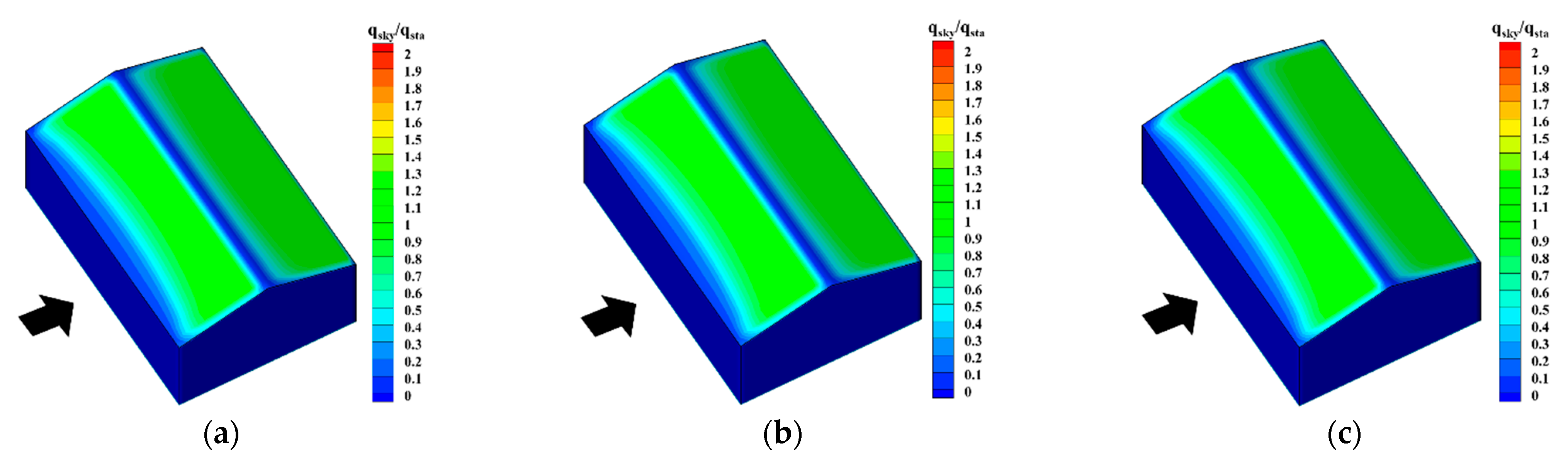
5.3. Impact of Snowfall Intensity

In addition to wind velocity, snowfall intensity is also one of the meteorological factors with strong randomness. To specify the impact of snowfall intensity on snow distribution on the gable roof, working conditions with three different snowfall intensities were set. The volume fractions of falling snow in three cases were set as 7.8 × 10⁻⁶, 1.56 × 10⁻⁵, and 2.34 × 10⁻⁵, which represented the snowfall intensity of 1.04 × 10⁻⁵ m/s (0.0375 m/h), 2.08 × 10⁻⁵ m/s (0.075 m/h), and 4.16 × 10⁻⁵ m/s (0.15 m/h), respectively. The wind velocity at the eave height was set as 5 m/s. The other computational settings are the same as above.

The spatial distributions of the volume fraction of falling snow and the friction velocity are the same for different cases. The typical results of the normalized volume fraction of falling snow α_sky/α_in and friction velocity $u_{*}/u_{*\mathrm{t}}$ are shown in Figure 18 and Figure 19, respectively. The falling snow particles are mainly concentrated downstream of both sides of the roof. Erosion occurs in the area in front of the ridge. Overall, the spatial distribution of falling snow and the aerodynamic erosion effect are little affected by the snowfall intensity. Figure 20 compares the spatial distribution of the normalized volume fraction of drifting snow α_surf/α_in with different snowfall intensities. Since the amount of drifting snow is mainly controlled by friction velocity, the absolute values of the volume fraction of drifting snow are the same too for different cases. The dimensionless values decrease with the increasing snowfall intensity, due to the increase in the denominator.

Figure 21 shows the spatial distribution of the normalized deposition flux of falling snow q_sky/q_sta with different snowfall intensities. The deposition flux is nearly the same in different cases. It indicates that the volume fraction of snow has little influence on the deposition flux caused by falling snow. The normalized friction velocities and normalized deposition flux of falling snow are nearly the same under different snowfall intensities; hence, the normalized deposition flux of drifting snow will not change much either, as shown in Figure 22. The normalized deposition flux of two kinds of snow phase keeps nearly unchanged with the increasing snowfall; however, from Equations (18) and (21), the normalized erosion flux decreases with the increase in snowfall intensity, due to the increase in the standard deposition flux q_sta. Therefore, the normalized snow depths decrease with the increasing snowfall intensity, as shown in Figure 23.

6. Conclusions

The study proposed a Eulerian–Eulerian approach for snow distribution, by considering the motions of different snow phases. Based on the validated approach, a series of CFD simulations are conducted to study the influence of snowfall conditions on snow loads on gable roofs. Finally, the following conclusions are derived:

• A multiphase approach was proposed and adopted in this paper to consider the transport process of falling and drifting snow, respectively. Furthermore, additional terms are inserted into the continuous equations of snow phases to simulate the processes of snow particles being trapped or ejected by snow surface. Through the comparison with the field measurement, it is proved that the proposed approach could well predict the snow distribution.
• As for the distribution characteristics, the falling snow particles in the air are easily affected by the high-speed airflow around the building and are generally evenly distributed outside the high-speed airflow area, and the distribution characteristics are less affected by the meteorological conditions. By contrast, the drifting snow is the main reason for the uneven distribution of snow on and around the building, and its distribution characteristics are much more sensitive to meteorological conditions.
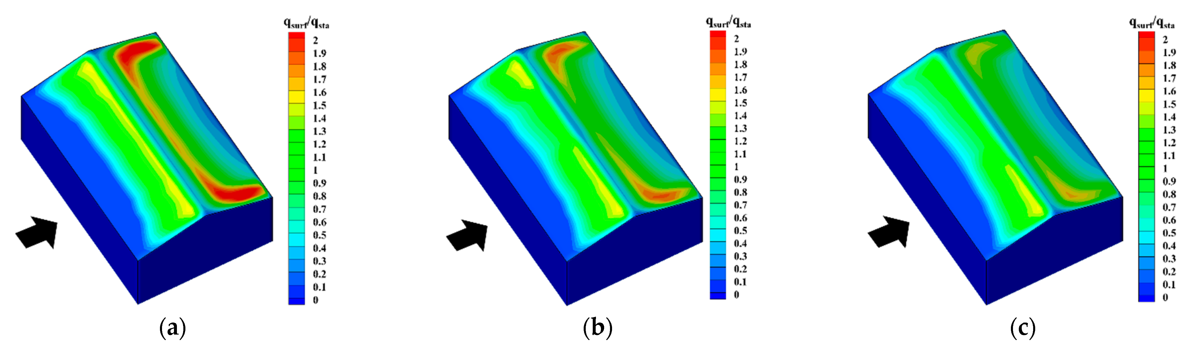
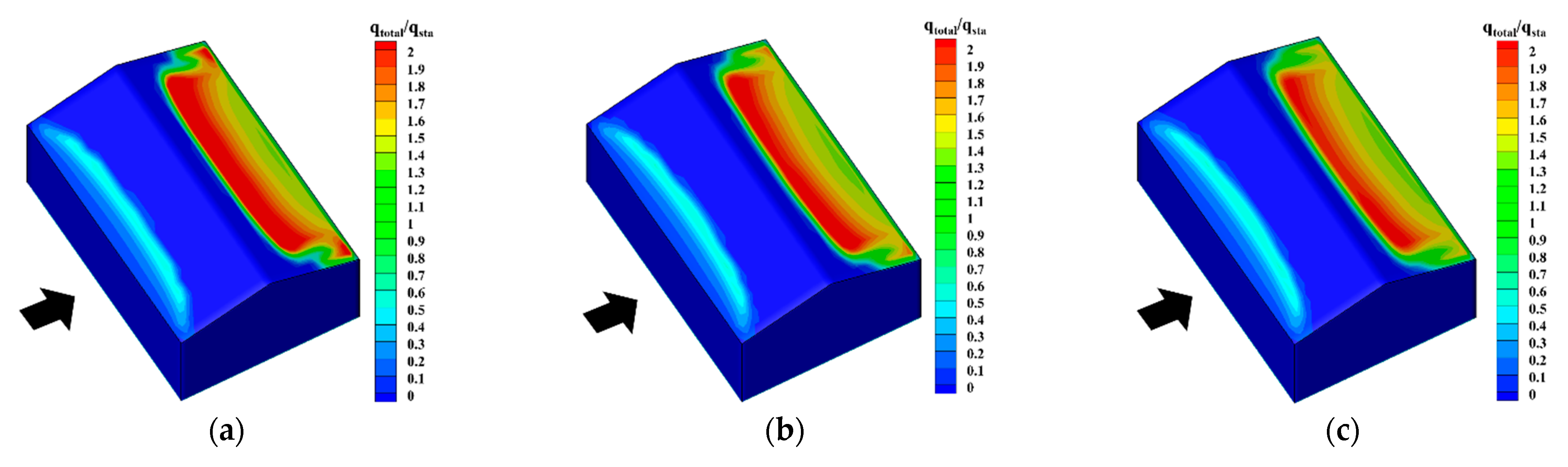
• The snowdrift patterns of gable roofs highly depend on the inflow wind velocity. When U_H ≤ 3 m/s, the snow distribution on the gable roof is generally even. When the wind velocity is between 3 m/s and 5 m/s, the snow distribution on the gable roof becomes uneven. When U_H > 5 m/s, snow distribution on the windward side nearly disappears, and the snow distribution on the leeward side is moved downstream further. Overall, the most adverse wind velocity range for this type of roof is between 3 m/s and 5 m/s.
• Snowfall intensity has less effect on snow distribution than inflow wind velocity. The friction velocity and normalized deposition of two kinds of snow phases are nearly not influenced by the increase in snowfall intensity. However, the normalized erosion flux decreases, due to the increase in the standard deposition flux; therefore, heavy snowfall intensity leads to more uniform snow distribution on the gable roof.

References

1. Tsuchiya, M.; Tomabechi, T.; Hongo, T. Wind effects on snowdrift on stepped flat roofs. J. Wind Eng. Ind. Aerodyn. 2002, 90, 1881–1892. [Google Scholar] [CrossRef]
2. Thiis, T.K.; Gjessing, Y. Large-scale measurements of snowdrifts around flat-roofed and single-pitch-roofed buildings. Cold Reg. Sci. Technol. 1999, 30, 175–181. [Google Scholar] [CrossRef]
3. Tominaga, Y. Computational fluid dynamics simulation of snowdrift around buildings: Past achievements and future perspectives. Cold Reg. Sci. Technol. 2018, 150, 2–14. [Google Scholar] [CrossRef]
4. Sun, X.Y.; He, R.J.; Wu, Y. Numerical simulation of snowdrift on a membrane roof and the mechanical performance under snow loads. Cold Reg. Sci. Technol. 2018, 150, 15–24. [Google Scholar] [CrossRef]
5. Uematsu, T.; Nakata, T.; Takeuchi, K. Three-dimensional numerical simulation of snowdrift. Cold Reg. Sci. Technol. 1991, 20, 65–73. [Google Scholar] [CrossRef]
6. Tominaga, Y.; Mochida, A. CFD prediction of flowfield and snowdrift around a building complex in a snowy region. J. Wind Eng. Ind. Aerodyn. 1999, 81, 273–282. [Google Scholar] [CrossRef]
7. Wang, Z.S.; Huang, N. Numerical simulation of the falling snow deposition over complex terrain. J. Geophys. Res.-Atmos. 2017, 122, 980–1000. [Google Scholar] [CrossRef]
8. Huang, N.; Wang, Z.S. The formation of snow streamers in the turbulent atmosphere boundary Layer. Aeolian Res. 2016, 23, 1–10. [Google Scholar] [CrossRef]
9. Lee, B.; Tu, J.; Fletcher, C. On numerical modeling of particle-wall impaction in relation to erosion prediction: Eulerian versus lagrangian method. Wear 2002, 252, 179–188. [Google Scholar] [CrossRef]
10. Tominaga, Y.; Okaze, T.; Mochida, A. CFD modeling of snowdrift around a building: An overview of models and evaluation of a new approach. Build. Environ. 2011, 46, 899–910. [Google Scholar] [CrossRef]
11. Okaze, T.; Mochida, A.; Tominaga, Y. CFD prediction of snowdrift around a cube using two transport equations for drifting snow density. In Proceedings of the 5th International Symposium on Computational Wind Engineering, Chapel Hill, NC, USA, 23–27 May 2010. [Google Scholar]
12. Kang, L.; Zhou, X.; Hooff, T. CFD simulation of snow transport over flat, uniformly rough, open terrain: Impact of physical and computational parameters. J. Wind Eng. Ind. Aerod. 2018, 177, 213–226. [Google Scholar] [CrossRef]
13. Zhou, X.; Kang, L.; Gu, M. Numerical simulation and wind tunnel test for redistribution of snow on a flat roof. J. Wind Eng. Ind. Aerod. 2016, 153, 92–105. [Google Scholar] [CrossRef]
14. Tominaga, Y.; Okaze, T.; Mochida, A. CFD simulation of drift snow loads for an isolated gable-roof building. In Proceedings of the 8th International Conference on Snow Engineering, Nantes, France, 14–17 June 2016. [Google Scholar]
15. Zhou, X.; Zhang, Y.; Gu, M. Coupling a snowmelt model with a snowdrift model for the study of snow distribution on roofs. J. Wind Eng. Ind. Aerod. 2018, 182, 235–251. [Google Scholar] [CrossRef]
16. Zhou, X.; Zhang, Y.; Kang, L. CFD simulation of snow redistribution on gable roofs: Impact of roof slope. J. Wind Eng. Ind. Aerod. 2019, 185, 16–32. [Google Scholar] [CrossRef]
17. Yu, Z.X.; Zhu, F.; Cao, R. Wind tunnel tests and CFD simulations for snow redistribution on roofs 3D stepped flat roofs. Wind Struct. 2019, 28, 31–47. [Google Scholar]
18. Zhang, G.L.; Zhang, Q.W.; Fan, F. Numerical Simulations of Development of Snowdrifts on Long-Span Spherical Roofs. Cold Reg. Sci. Technol. 2021, 182, 103–211. [Google Scholar] [CrossRef]
19. Zhang, G.L.; Zhang, Q.W.; Fan, F. Numerical simulations of snowdrift characteristics on multi-span arch roofs. J. Wind Eng. Ind. Aerod. 2021, 212, 104593. [Google Scholar] [CrossRef]
20. Yin, Z.; Zhang, Q.; Zhang, G. CFD investigations of interference effects of building groups with flat roofs on snow load. Cold Reg. Sci. Technol. 2021, 191, 103371. [Google Scholar] [CrossRef]
21. Yin, Z.; Zhang, Q.; Zhang, G. CFD simulations of interference effects of two low-rise buildings on snow load. Cold Reg. Sci. Technol. 2022, 199, 103577. [Google Scholar] [CrossRef]
22. Zhang, Q.; Zhang, G.; Yin, Z. Experimental Study of Interference Effects of a High-Rise Building on the Snow Load on a Low-Rise Building with a Flat Roof. Appl. Sci. 2021, 11, 11163. [Google Scholar] [CrossRef]
23. Zhang, G.L. Study on Numerical Simulation Approach of Snowdrifts and Snow Load Characteristics on Long-Span Roofs. Ph.D. Thesis, Harbin Institute of Technology, Harbin, China, 2021. (In Chinese) [Google Scholar] [CrossRef]
24. Oikawa, S.; Tomabechi, T. Daily observation of snowdrifts around a model cube. In Snow Engineering; Hjorth-Hansen, H., Loset, N., Eds.; Balkema: Rotterdam, The Netherlands, 2000. [Google Scholar]
25. Okaze, T.; Mochida, A.; Tominaga, Y. Modeling of drifting snow development in a boundary layer and its effects on wind field. In Proceedings of the 6th International Conference on Snow Engineering, Nantes, France, 14–17 June 2016. [Google Scholar]
26. Tominaga, Y.; Mochida, A.; Yoshie, R. AIJ guidelines for practical applications of CFD to pedestrian wind environment around buildings. J. Wind Eng. Ind. Aerodyn. 2008, 96, 1749–1761. [Google Scholar] [CrossRef]
27. AIJ. AIJ Recommendations for Loads on Buildings; AIJ: Tokyo, Japan, 2004. [Google Scholar]
Figure 1. Incident profiles of the flow field (a) normalized streamwise velocity; (b) normalized turbulence kinetic energy; (c) turbulent dissipation rate.
Buildings 12 01878 g001
Figure 2. Computational domain and boundary conditions.
Buildings 12 01878 g002
Figure 3. Computational grids: (a) coarse mesh, 231,400 hexahedral cells with the minimum size being 0.05 H (y+ = 250); (b) basic mesh, 789,725 hexahedral cells with the minimum size being 0.04 H (y+ = 200); (c) fine mesh, 2,264,744 hexahedral cells with the minimum size being 0.015 H (y+ = 75).
Buildings 12 01878 g003
Figure 4. Streamwise velocity along seven vertical lines at a center vertical section for different meshes.
Buildings 12 01878 g004
Figure 5. Stream lines at the top of the cube for three meshes: (a) coarse mesh; (b) basic mesh; (c) finer mesh.
Buildings 12 01878 g005
Figure 6. Streamwise velocity along seven horizontal lines at a horizontal section.
Buildings 12 01878 g006
Figure 7. Settings of the computational domain.
Buildings 12 01878 g007
Figure 8. Normalized deposition flux of two types of snow phases and erosion flux: (a) normalized deposition flux of drifting snow; (b) normalized deposition flux of falling snow; (c) normalized erosion flux.
Buildings 12 01878 g008
Figure 9. Normalized snow depth of the numerical simulation.
Buildings 12 01878 g009
Figure 10. Comparison of numerical simulations and field measurement: (a) streamwise direction; (b) lateral direction.
Buildings 12 01878 g010
Figure 11. Cell generation of the gable roof: (a) ground and building surfaces; (b) central section of the building.
Buildings 12 01878 g011
Figure 12. Normalized volume fraction of falling snow αskyin around the gable-roofed building: (a) UH = 2 m/s; (b) UH = 3 m/s; (c) UH = 4 m/s; (d) UH = 5 m/s; (e) UH = 6 m/s; (f) UH = 7 m/s.
Buildings 12 01878 g012
Figure 13. Normalized friction velocity u * / u * t : (a) UH = 2 m/s; (b) UH = 3 m/s; (c) UH = 4 m/s; (d) UH = 5 m/s; (e) UH = 6 m/s; (f) UH = 7 m/s.
Buildings 12 01878 g013
Figure 14. Normalized volume fraction of drifting snow αsurfin: (a) UH = 2 m/s; (b) UH = 3 m/s; (c) UH = 4 m/s; (d) UH = 5 m/s; (e) UH = 6 m/s; (f) UH = 7 m/s.
Buildings 12 01878 g014aBuildings 12 01878 g014b
Figure 15. Normalized deposition flux of falling snow qsky/qsta: (a) UH = 2 m/s; (b) UH = 3 m/s; (c) UH = 4 m/s; (d) UH = 5 m/s; (e) UH = 6 m/s; (f) UH = 7 m/s.
Buildings 12 01878 g015aBuildings 12 01878 g015b
Figure 16. Normalized deposition flux of drifting snow qsurf/qsta: (a) UH = 2 m/s; (b) UH = 3 m/s; (c) UH = 4 m/s; (d) UH = 5 m/s; (e) UH = 6 m/s; (f) UH = 7 m/s.
Buildings 12 01878 g016
Figure 17. Normalized total deposition flux qtotal/qsta: (a) UH = 2 m/s; (b) UH = 3 m/s; (c) UH = 4 m/s; (d) UH = 5 m/s; (e) UH = 6 m/s; (f) UH = 7 m/s.
Buildings 12 01878 g017aBuildings 12 01878 g017b
Figure 18. Normalized volume fraction of falling snow αskyin around the gable-roofed building.
Buildings 12 01878 g018
Figure 19. Normalized friction velocity u * / u * t .
Buildings 12 01878 g019
Figure 20. Normalized volume fraction of drifting snow αsurf/αin on the gable roof: (a) volume fraction: 7.8 × 10⁻⁶; (b) volume fraction: 1.56 × 10⁻⁵; (c) volume fraction: 2.34 × 10⁻⁵.
Buildings 12 01878 g020
Figure 21. Spatial distribution of the normalized deposition flux of falling snow qsky/qsta with different snowfall intensities: (a) volume fraction: 7.8 × 10⁻⁶; (b) volume fraction: 1.56 × 10⁻⁵; (c) volume fraction: 2.34 × 10⁻⁵.
Buildings 12 01878 g021
Figure 22. Spatial distribution of the normalized deposition flux of drifting snow qsurf/qsta with different snowfall intensities: (a) volume fraction: 7.8 × 10⁻⁶; (b) volume fraction: 1.56 × 10⁻⁵; (c) volume fraction: 2.34 × 10⁻⁵.
Buildings 12 01878 g022
Figure 23. Spatial distribution of the normalized total deposition flux qtotal/qsta with different snowfall intensities: (a) volume fraction: 7.8 × 10⁻⁶; (b) volume fraction: 1.56 × 10⁻⁵; (c) volume fraction: 2.34 × 10⁻⁵.
Buildings 12 01878 g023