Effects of the Built Environment on Travel-Related CO₂ Emissions Considering Travel Purpose: A Case Study of Resettlement Neighborhoods in Nanjing

Abstract

With rapid urbanization, an increasing number of resettlement housing neighborhoods have been developed in suburbs in China. Such neighborhoods often face problems of spatial mismatch (jobs–housing and daily life), excessive street scale, and inconvenient transportation, which directly and indirectly lead to long travel distances and higher travel carbon emissions for residents. Understanding how to improve the built environment of resettlement housing and thus influence travel CO₂ emissions is essential to guide low-carbon travel and reduce greenhouse gas emissions. Based on an electronic questionnaire and travel carbon emission measurements collected in 12 resettlement housing neighborhoods in Nanjing in 2022, this study used a three-group structure equation model (SEM) to measure the impact of resettlement housing’s built environment on travel CO₂ emissions from commutes, housework trips, and recreational trips. It was found that the improvement of destination accessibility can significantly reduce the carbon emissions of residents’ trips. Second, the built environment of resettlement housing can affect travel carbon emissions through mediator variables and direct effects. In addition, these effects show different paths and sizes depending on the purpose of the travel trip. These results are significant for the planning and construction of resettlement houses and offer guidance for low-carbon travel.

1. Introduction

Transportation-related greenhouse gas (GHG) emissions, especially CO₂ emissions, are one of the most pressing issues in the context of global warming and climate change [1]. There are three main factors influencing the carbon emissions of urban transport: travel behavior (e.g., travel distance, travel mode choice), urban space (e.g., urban form, land use, street design), and transportation carbon technologies (e.g., vehicle technology and fuel technology) [2,3,4]. In urban planning, research focusing on improving urban spatial structure and optimizing land-use patterns, thus reducing travel demand, changing travel behavior, and reducing carbon emissions to combat climate change, has attracted considerable attention [5,6,7].

Rapid urbanization in China has brought about constant renewal in the city centers and rapid suburban expansion. Generally speaking, to use land efficiently, houses with well-positioned locations and convenient transportation but poor living environments in the city centers have been demolished by the government. The residents have been relocated to houses in the suburbs, called resettlement housing. As marginalized urban living spaces, these resettlement housing neighborhoods face problems: spatial mismatch (jobs–housing and daily life), excessive street scale, and transportation difficulties [8,9]. For example, regarding commutes, John Kain’s spatial mismatch hypothesis suggests that restricted housing options can limit people’s access to optimum jobs [10], which means more cars and travel carbon to offset this effect. Another study has shown that street scale and active travel facilities can impact travel carbon emissions [11]. Moreover, poorer facilities and lower accessibility of public service facilities may lead to higher carbon emissions [12]. In addition, several studies on travel carbon emissions at the urban level also show that people living in suburban areas tend to use more motorcars [13]. Therefore, it is essential to discuss the impact of built environments in resettlement areas on people’s travel behavior and carbon emissions.

2. Theoretical Background

Research on the built environment, travel behavior, and carbon emissions from travel has focused on studying the interaction between the two. Travel behavior, such as travel mode, distance, purpose, and frequency, influences travel carbon emissions. Among these, travel mode and travel distance, as the most critical factors, directly affect travel carbon emissions, while carbon emission factors measured for different travel modes are also proliferating [14,15,16]. As for travel purposes, a study in Baltimore found that the built environment has a different impact on vehicle miles traveled (VMT) and vehicle energy consumption between commuting and non-commuting trips [17]. A study in Guangzhou, China, discussed the impact of the built environment of community dimensions on travel carbon emissions for different trip purposes, including commuting trips, social trips, recreational trips, and daily shopping trips [15,18]. In addition, the studies concluded that residents who traveled longer distances had higher travel carbon emissions, while those who traveled more times in a day and used more low-carbon modes (including walking, bicycle, bus, and subway) had lower travel carbon emissions [19].

Many studies have examined the relationship between the built environment and travel behavior, among which Cervero and Kockelman in 1997 first proposed the use of “3D” to assess the built environment, namely, “density,” “diversity,” and “design” [20]. On this basis, “destination accessibility” and “distance to transit” were added for the “5D“ [21]. Most research about travel behavior focuses on travel mode choice, travel distance, travel frequency, and VMT. There are some commonalities, although the conclusions of these studies are not entirely consistent. For example, in areas with higher population and building density, due to the proximity of origins to destinations and the prevalence of better public transportation services, travel distances are likely to be reduced, and travel modes may shift to non-motorized modes [22]. In terms of trip frequency, the study concluded that the frequency of non-commute activities decreases primarily with the increasing travel distance [23]. For personal VMT, a study of the Baltimore metropolitan area concluded that the residential built environment has a significant impact on VMT for commute and non-commute trips, primarily in terms of employment density, land-use mixture, street connectivity, and accessibility [17]. However, the above studies pay little attention to the environmental costs, such as travel carbon emissions, which are also intimately related to the urban built environment and residents’ travel [18,24].

From the relationship between built environment and travel behavior, scholars have started to use travel behavior as a mediator to study the relationship between the built environment and carbon emissions from travel. In terms of density, Gim’s study on the international scale concluded that higher population density in high-density built-up areas, along with compact development in urban cores, reduces travel, indirectly reducing travel CO₂ emissions [25]. Cao and Yang’s study on Guangzhou concluded that residential density negatively affects CO₂ emissions from commuting but positively affects CO₂ emissions from social, recreational, and daily shopping trips [18]. In addition, studies on the non-linear relationship between density and travel-related carbon emissions have emerged in recent years. Hong noted that the impact of increasing residential density on reducing travel carbon emissions would be insignificant when the residential density reaches a certain level [26]. A study by Liu et al. in Norway pointed out that household transportation carbon emissions show an inverted U-shape relationship with building density [24].

Diversity is commonly measured using land-use mixture, which significantly impacts travel carbon emissions. Cervero found that more intensive and higher mixed development can promote the use of transit and non-motorized modes of travel [21]. A study by Liu et al. in Beijing found that residents living in higher land-use mixtures tended to use “low-carbon” travel modes (i.e., walking, bicycle, bus, and subway) and emit less CO₂ on their daily trips [19]. The Minneapolis-St. Paul Metropolitan Area study by Wu et al. used the land-use entropy index to measure diversity and concluded that the land-use entropy index was negatively correlated with travel CO₂ emissions over a range of values [27].

Direct research on design and travel carbon emissions remains scarce, and the focus of relevant studies is still on the traditional effects of road network density and road crossing density on travel behavior, lacking consideration of walking and cycling environments. Studies have shown that the slow traffic system, specifically, pedestrian-friendly roadway design (e.g., traffic calming, sidewalk shading), can reduce car trips and increase walking, biking, and transit travel [20,23], but there is a lack of discussion on travel-related carbon emissions. A study in Albuquerque, USA, found that bicycle facilities can increase the bicycle mode share and reduce the use of driving by influencing those with less cycling experience. However, this study did not address the impact on travel carbon emissions [28].

Destination accessibility (DA) has an impact on people’s travel behavior. Accessibility is an important predictor of VMT, car ownership, travel mode choice, and mode share [29,30]. A study in Greater Montreal found that both local and regional accessibility had a statistically negative association with driving choice and vehicle distance driven by drivers [31]. A study of Guangzhou, China concluded that residents of newly developed urban areas and remote districts with lower population and employment density, along with poorer accessibility to facilities and services, produce more CO₂ emissions during the workday [12]. However, some studies have argued that an increase in facility accessibility, i.e., a reduction in the average distance to a facility, may result in more travel demand, and the net influence is uncertain [23,32].

There is a quantitative relationship between public transport accessibility (PTA) and travel-related CO₂ emissions. Research by Ashik et al. on Dhaka, the capital of Bangladesh, concluded that a high-quality public transport system and shorter distance to transit stops could reduce CO₂ emissions indirectly by reducing car ownership [33]. A study in Beijing, China, concluded that residents with higher retail density, subway accessibility, and low-speed street density tend to emit less CO₂ in their daily travel [19]. There are also research findings that public transit services have no quantitative relationship with travel-related CO₂ emissions. A study in Beijing and Xi’an concluded that metro stations within 500 m of the household location were not statistically significant in reducing commuting CO₂ emissions [13].

It is worth mentioning that the variation in findings across studies for the same variables has been attributed to “Residential self-selection (RSS)”. RSS refers to people’s choice of residential location based on travel demand, travel ability, and travel preference. For example, residents who prefer to travel by walking choose to live in a walkable environment rather than a non-walkable environment, creating residents who like walking [34]. Along with the changing housing supply market and affordability of residents, a growing number of studies have considered residential self-selection. For our research, however, unlike commercial housing, the housing locations and environments are built by government-led construction in resettlement housing residential locations, which means residents have a smaller degree of RSS. Therefore, this study did not include RSS as a point of discussion.

The aforementioned studies did not consider resettlement housing. Furthermore, their focus was primarily on general residential areas, most of which were in main city areas. For instance, a study in Beijing and Xi’an, China, concluded that residents living in the outer suburbs had the lowest travel CO₂ emissions, while those living in the inner suburbs had the highest travel CO₂ emissions [13], which did not involve the classification of residential spaces and populations. However, even for suburban residential neighborhoods, travel mode choices are often related to residential self-selection effects and affordability, especially for ordinary commercial housing. The results for resettlement neighborhoods, government-led construction, and less selective locations are often not representative.

In conclusion, although existing studies discuss the relationship between the built environment, travel behavior, and travel-related carbon emissions, they primarily focus on discussing ordinary residential neighborhoods in main city areas. Taking Nanjing city as a case study, we investigated the relationship between the built environment, travel behavior, and travel carbon emissions around the three issues of resettlement housing neighborhoods. A three-group structural equation model (SEM), grouped by commutes, housework trips, and recreational trips, was used to analyze the direct effects (DE), indirect effects (IE), and total effects (TE) of research content. The built environment was divided into density, diversity, satisfaction with slow traffic system (SSTS), destination accessibility (DA), and public transport accessibility (PTA). Among these, SSTS represents residents’ feelings about the street scale, DA shows the spatial mismatch of neighborhoods, and PTA indicates the convenience of travel. This is the difference between our research and similar studies.

The remainder of this paper is structured as follows: The second section presents the data, methodology, and theoretical framework. The model results are explained in the third section. The last section discusses the main conclusions of the study and the corresponding policy recommendations.

3. Materials and Methods

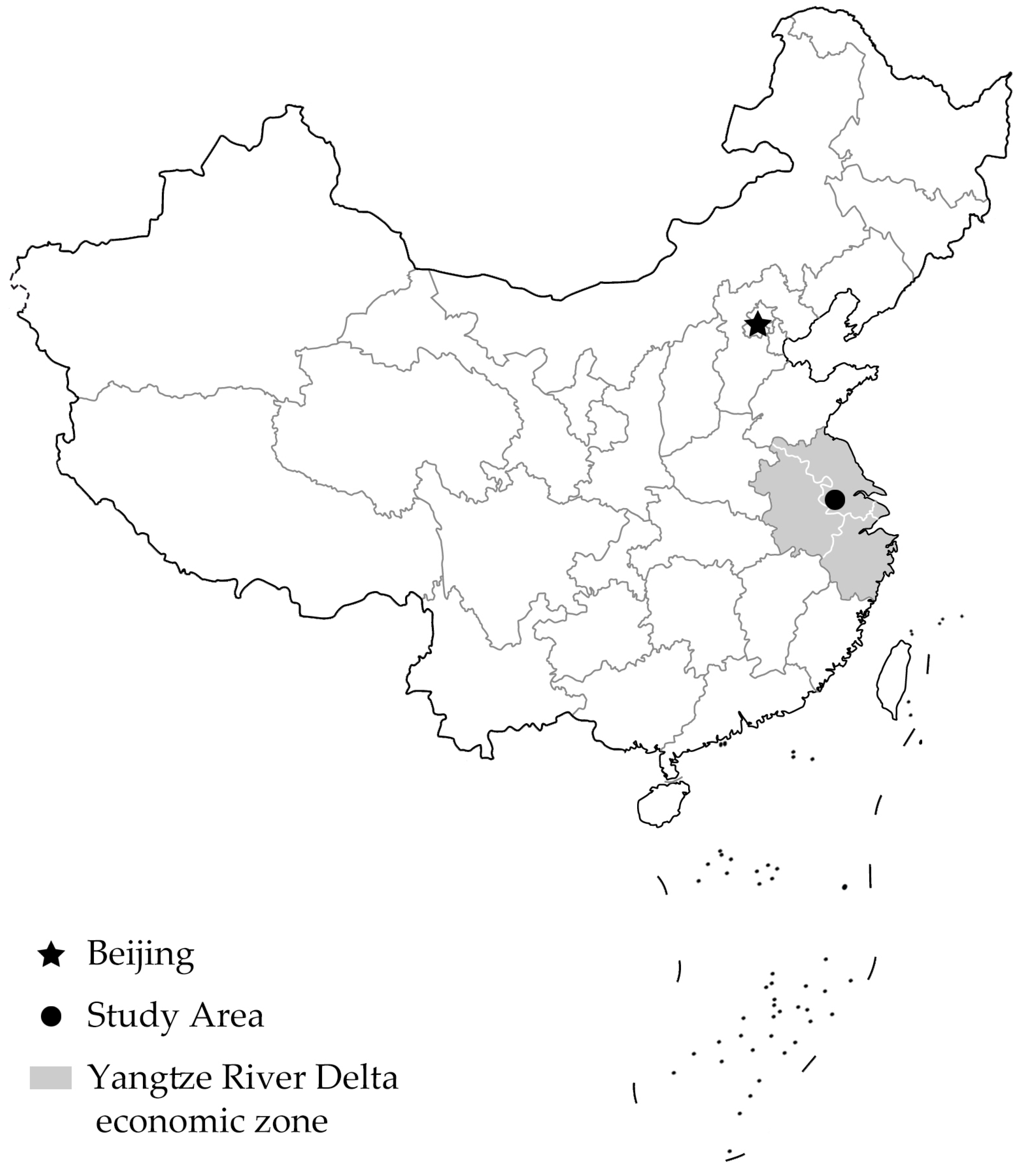
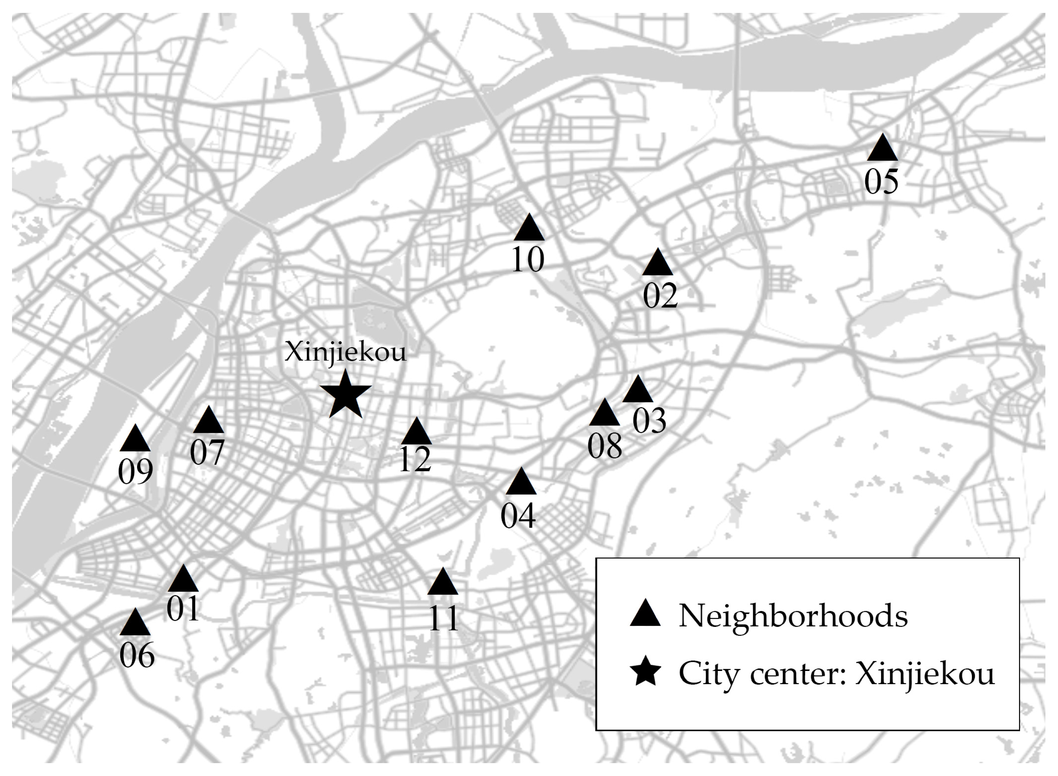
3.1. Study Area and Neighborhoods Surveyed

The city of Nanjing was used as the case city in this research. Unlike Western countries, China’s suburban residential resettlement pattern tends to place demolished residents, poor people with housing difficulties, and people with relatively low incomes in suburban areas [35]. The same pattern exists in Nanjing, the capital of Jiangsu Province and the core city of China’s Yangtze River Delta economic zone (Figure 1). With the accelerated renewal process of the old city and the continuous expansion of urban space, the scale of resettlement housing construction in Nanjing has gradually increased since 2002. The completed area of affordable housing, mainly resettlement houses and public rental houses, has increased from 0.2 million square meters in 2002 to 2.08 million square meters in 2020. Twelve resettlement neighborhoods were selected based on different construction years, locations, and built environments for our study. Their locations are shown in Figure 2. The construction year and built environment indicators of each neighborhood are shown in

Table 1. Basic characteristics of surveyed neighborhoods.

ID	Name	Year of Construction	Building Form	PD	LUM	DTMS	BSD	Valid Samples
01	Lian Hua Xin Cheng	2000 (Jia Yuan) 2005 (Bei Yuan) 2012 (Nan Yuan)	HA	10,010.83	0.19	627.67	6.80	32
02	Xian Lin Xin Cun	2001	MA	6676.29	0.16	879.00	9.95	28
03	Bai Shui Qian Cheng, Bai Shui Jia Yuan	Shang Shui Fang (2003) Chun Shui Fang (2003) Bai Shui Jia Yuan (2004) Yun Shui Fang (2007)	MA	7029.53	0.24	1754.50	3.98	26
04	Yin Long Hua Yuan	2004 (Phase I) 2005 (Phase II)	MA	6355.23	0.18	4462.00	2.99	31
05	She Shan Xing Cheng	2005 (Ting Zhu Yuan) 2007 (Shang Ju Yuan)	MA	3387.50	0.22	1253.00	5.97	48
06	Dai Shan Qi Xiu Bei Yuan, Dai Shan Qi Xiu Nan Yuan	2008 (Bei Yuan) 2010 (Nan Yuan)	HA	3126.14	0.18	986.00	6.22	36
07	Jia He Yuan	2009	HA	7520.09	0.27	572.00	7.96	39
08	Sheng He Jia Yuan	2012	HA	2678.14	0.18	2962.00	4.48	29
09	Zhou Dao Jia Yuan, Zhou Dao He Yuan	2014 (Zhou Dao Jia Yuan) 2015 (Zhou Dao He Yuan)	HA	1361.86	0.24	3539.50	2.49	42
10	Ding Jia Zhuang Hui Jie Xin Cheng	2016	HA	5104.24	0.18	3215.00	4.48	52
11	Qin Wan Jing Yuan	2017	HA	4245.36	0.18	945.00	3.98	27
12	Yu Dao Jia Ting	2020	HA	34,165.59	0.17	542.00	6.97	28

Note: HA is high-rise apartments; MA is multistory apartments; population density (PD) is measured in 10,000 persons/km²; distance to the nearest metro station (DTMS) is measured in km; bus stop density (BSD) is measured in counts /km².

. As can be seen from the table, the year of construction of the 12 resettlement housing neighborhoods are all after 2000. Among them, a greater number of neighborhoods were built from 2003 to 2007, which is consistent with the period of large-scale construction of affordable housing in Nanjing. It is worth mentioning that the construction of resettlement housing in Nanjing generally takes the pattern of batch construction, which means differences in the geographical location and the built environment of resettlement house neighborhoods in different construction years. For example, Lian Hua Xin Cheng, built in 2000, is located in the southwest of the main city of Nanjing, which has a higher population density, better facilities for daily life, and public transportation. As for the building form, most of the buildings before 2008 were multistory apartments, while the resettlement housing complexes built after 2008 were high-rise apartments. To ensure the representativeness of the surveyed neighborhoods for built environment indicators, our research used population density (PD), land-use mixture (LUM), distance to the nearest metro station (DTMS), and bus stop density (BSD) for 12 resettlement housing communities. The neighborhood nearest to the city center (No. 12) had the highest population density in the survey, and the one located on Nanjing’s Jiangxin Island (No. 09) had the lowest population density. Regarding land use, Xian Lin Xin Cun, located in Xian Lin university town and 15 km from the city center (Xinjiekou), has the lowest mixture of land use; Jia He Yuan, with the highest mixture of land use, is 5.5 km from Xinjiekou, with ample commercial facilities around the community, including Wanda Plaza, Suning Huigu, and other commercial shopping squares. More than half of the neighborhoods are within 1.5 km of the path distance from the subway station, and the average density of bus stops is 5.5/km². In general, represented by PD, LUM, DTMS, and BSD, there are some differences in the built environment of these 12 resettlement housing neighborhoods. The diversity of the built environment makes it more beneficial to quantify the impact of the built environment on travel-related CO₂ emissions in Section 4.

The survey was conducted in June and July 2022. We used an electronic questionnaire for sample selection using random face-to-face sampling on the street. The questionnaire included three aspects of travel behavior, neighborhood built environment scores, and personal socioeconomic attributes. Finally, 424 questionnaires were collected, and 418 valid questionnaires were obtained after data collation. In addition, each questionnaire was collected for three trip purposes: commute, housework trips and recreational trips, which received 409, 365, and 339 valid origin–destination (OD) data separately, totaling 1113 travel data. Details of the individual socioeconomic attributes of the sample are shown in

Table 2. Distribution of socioeconomic attributes for sample.

Variable	Level	Frequency	Percentage
Gender	male	180	43.06%
	female	238	56.94%
Age	≤20	7	1.67%
	20–30	130	31.10%
	30–40	131	31.34%
	40–50	89	21.29%
	50–60	44	10.53%
	>60	17	4.07%
Household size	1–2	94	22.49%
	3–4	257	61.48%
	≥5	67	16.03%
Employed size in household	1–2	309	73.92%
	3–4	103	24.64%
	≥5	6	1.44%
Any child under 18	Yes	220	52.63%
	No	198	47.37%
Education	Senior high school and below	99	23.68%
	Junior college	119	28.47%
	Bachelor/Master degree	200	47.85%
Occupation	Government or institutional employees	54	12.92%
	Corporate management/technical employees	122	29.19%
	Corporate logistics employees	71	16.99%
	Service industry employees	35	8.37%
	Self-employed	15	3.59%
	Freelancers	57	13.64%
	Students	14	3.35%
	Non-working/retired	50	11.96%
Length of residence	Less than 1 year	52	12.44%
	1–3 years	89	21.29%
	3–5 years	74	17.70%
	5 years or longer	203	48.56%
Personal monthly income	≤2500 CNY	58	13.88%
	2500–5000 CNY	138	33.01%
	5000–10,000 CNY	141	33.73%
	10,000–15,000 CNY	52	12.44%
	15,000–20,000 CNY	16	3.83%
	>20,000 CNY	13	3.11%
Car ownership	0 car	118	28.23%
	1 car	258	61.72%
	2 cars	37	8.85%
	>2 cars	5	1.20%
Preference for car travel	Yes	39	9.33%
	No	379	90.67%
Bike/E-bike ownership	Yes	332	79.43%
	No	86	20.57%

. The sample was generally balanced in terms of gender distribution, with the largest age group amount being the 30–40 year-old range and more than 50% of respondents having education below a bachelor’s degree. Over 77% of respondents reported a household size of three or more, while nearly three-quarters had only one to two employed persons in their families. Occupations were widely distributed, with the largest number of groups being corporate management/technical employees and corporate logisticians; more than 80% of residents had a monthly personal income of less than CNY 10,000 (official currency of the People’s Republic of China); nearly 70% of residents owned private cars, but only 10% of respondents said they preferred to travel in cars.

3.2. Variables and Data

The data in this study were divided into individual travel behavior, travel carbon emissions, and built environment. The sources of data and their characteristics are described as follows:

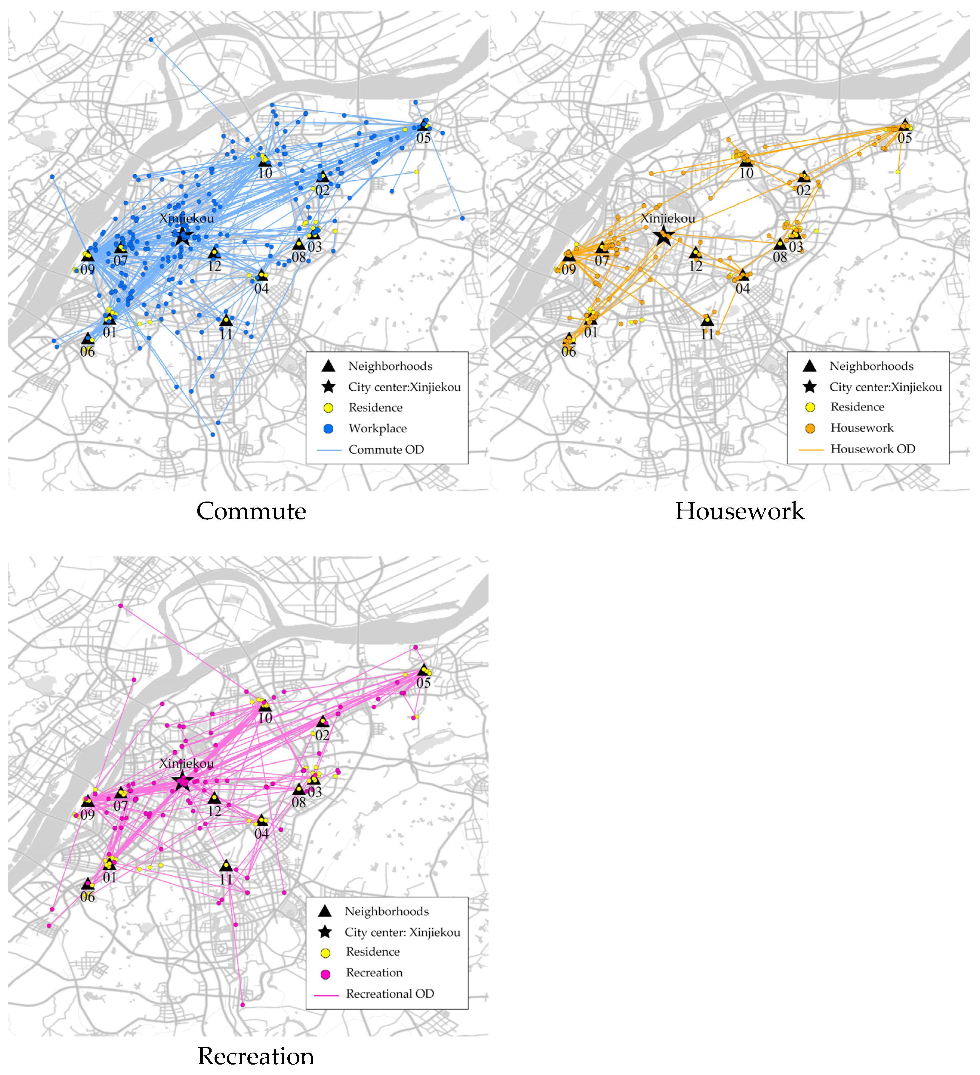
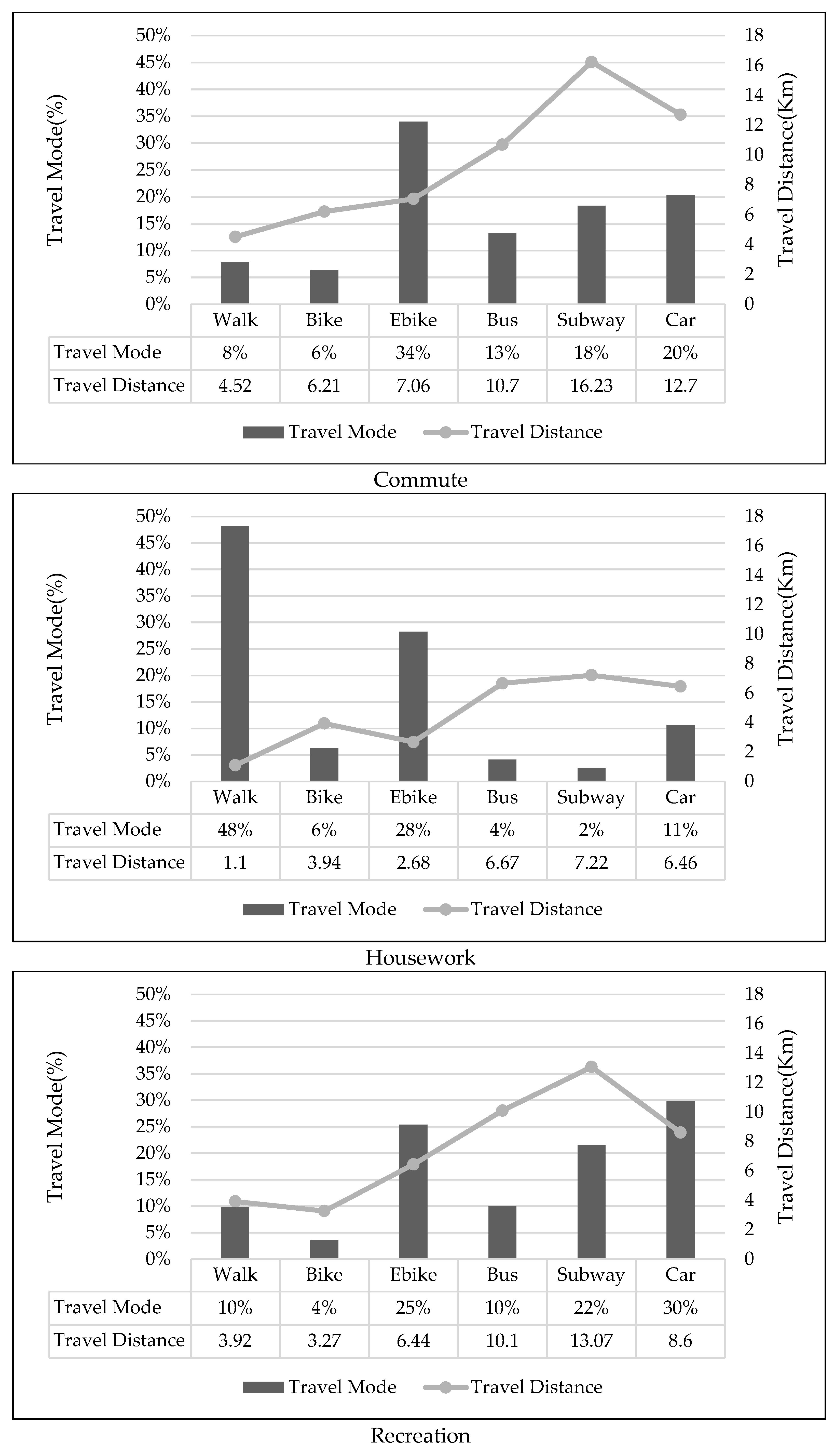
3.2.1. Travel Behavior

According to the addresses of residential neighborhoods and three types of travel destinations obtained from the questionnaire, the corresponding latitude and longitude were collected through the Amap open platform geocoding application programming interface (API). The surrounding search API was used to correct the unclear addresses through the Python program. The final travel OD flows were obtained as shown in Figure 3. Respondents’ workplaces were concentrated in the city center, but relatively evenly distributed overall. Similarly, recreational destinations were mostly located in the city center, but with a more obvious trip centripetal. Housework destinations were mostly distributed around the residential neighborhood, and there were a few long-distance trips.

The individual travel distances were obtained through the route search API of the Amap open platform based on the longitude and latitude of the travel origin and destination, which is more accurate than using the straight-line distance to characterize the travel distance. As for the travel modes, we took six types of travel modes commonly used by residents in China: walking, bike (including private and public bikes), e-bike, bus, subway, and car (including private car, taxi, and car-hailing services). Among the six travel modes, all except the car were defined as low-carbon travel modes, which is consistent with the definition of related low-carbon travel studies [19,36,37].

It is worth mentioning that although vehicle energy transitions are included as an important study in some low-carbon travel studies, our research does not make a distinction based on the difference in energy use by motor vehicles. There are two reasons for this: first, according to the Nanjing Statistical Yearbook 2021, by the end of 2020, the number of cars in Nanjing was 1,737,600, of which 54,200 were new energy vehicles (including electric cars and hybrid power cars), accounting for only 3% of the total [38,39]. High-carbon emission vehicles powered by fossil fuels still remain the primary choice for people with small cars. Therefore, to simplify the calculation, the car mode discussed in this research includes cars of various energy sources.

The percentage of travel mode and the average distance of travel for the three travel purpose samples are shown in Figure 4. For commuting, the most popular travel mode used by residents of resettlement house neighborhoods was e-bikes, accounting for more than one-third of the commute sample, followed by cars and subways, accounting for 20% and 18%, respectively. The average travel distance for the commuter sample was 10.11 km, the highest percentage of e-bike travel was lower than the total sample at 7.06 km, and the subway had the farthest average travel distance at 16.23 km.

Housework travel was dominated by walking (48%) and e-bikes (28%), with an overall average travel distance of 2.68 km. The average distance for all six modes of household travel was lower than the average travel distance in commute. The subway (7.22 km) was at the top of the list of average travel distances, while buses (6.67 km) and cars (6.46 km) had travel distances close to the subway. It can be seen that a higher proportion of people choose low-carbon travel modes for housework trips, but there are some motorized trips with slightly longer travel distances.

For recreational trips, cars (including taxis) (30%), e-bikes (25%), and subways (22%) were dominant. The average travel distance for recreation was 8.52 km, between the average commute distance and housework trips. Among them, the subway still had the longest average travel distance, reaching 13.07 km, but was lower than the average travel distance for commutes.

For all six modes, walking (48%) accounted for the highest percentage of housework trips, e-bikes (34%) were used for the highest percentage of commutes, and cars (30%) tended to be used more for recreational trips. The proportion of bikes for the three travel purposes was basically equal, and the ratio of bus and subway use was closer for commute and recreation, which shows that the people using these three modes are more fixed. The difference in travel mode choice between the three travel purposes may be related to the varying demands of residents. Studies show that people care more about travel time and efficiency when traveling [40]. Not only can e-bikes move faster on congested city streets during peak hours in the morning and evening, avoiding the crowds of public transportation, but they are also more physically efficient than walking and biking. For housework, as shown in Figure 3, residents’ housework travel destinations were generally located around their homes, as it is more convenient to walk and e-bike. Those residents who make recreational trips prefer to travel by car with a higher level of comfort. In addition, even if the comfort level is inferior to the car, people are willing to travel by e-bike due to the convenience, compact size, and money-saving features, as well as people’s preference in travel mode. Overall, there are differences in travel mode choices for different travel purposes, which provides a theoretical basis for the subsequent research in this study using travel mode as a mediator variable.

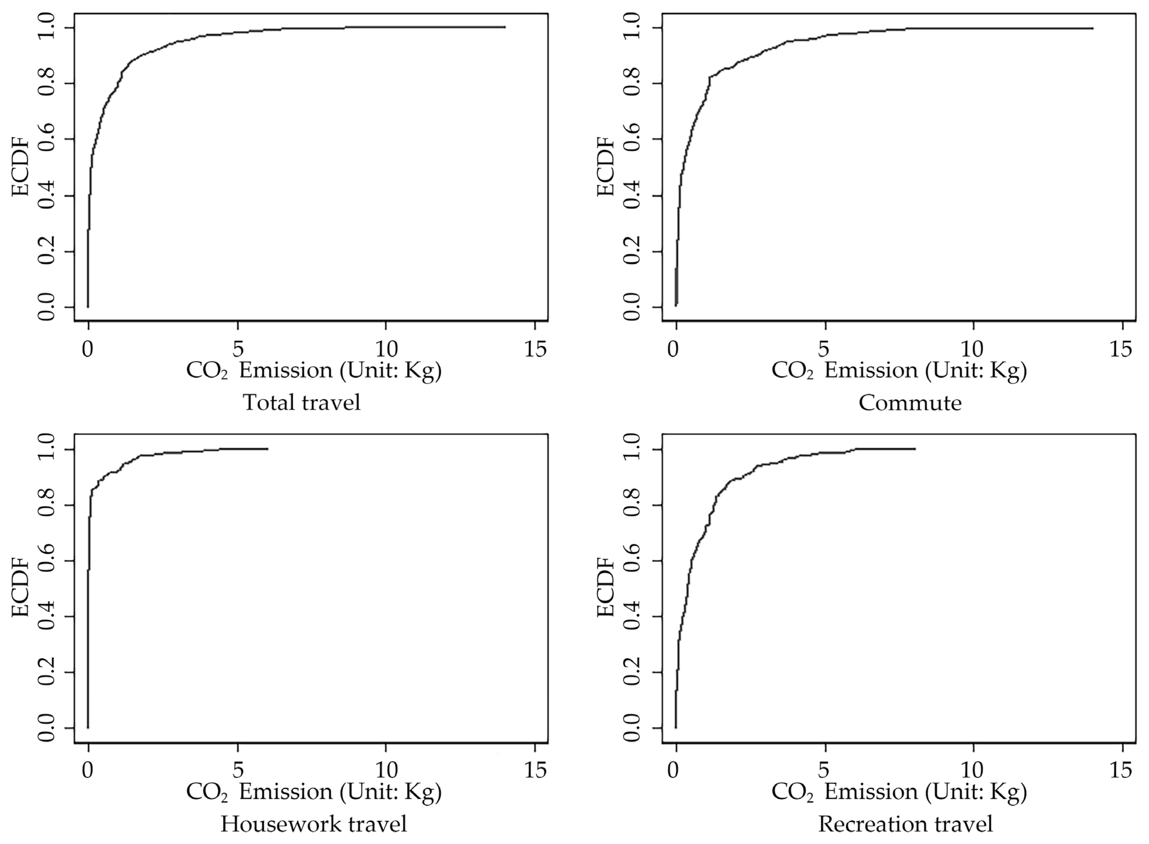
3.2.2. Travel-related CO₂ emissions

Referring to existing studies involving carbon emissions from travel [12,13,19,41,42], we applied the following formula to calculate the personal CO₂ emissions from a single trip of the sample:

$$Carbon=D\times E{F}_m$$

where: $Carbon$ denotes personal CO₂ emissions for a single trip (kgCO₂/Person), $D$ indicates travel distance (Km), and $E{F}_m$. is the travel emissions factor based on different travel modes (kgCO₂/ PKM). Even if a single trip involved more than one travel mode, to simplify the calculation, we took the main travel mode for a single trip mode. The main travel mode here refers to the mode that residents used for the longest distance in a single trip, and we asked respondents to choose it in the questionnaire. In addition, according to Wallner et al., when residents use cars to commute on a single trip, they usually do not use active travel and public travel modes at the same time [43]. Moreover, when public transportation is the main mode, people walk between public transportation stations, and in most conditions, use only a single public transportation service [43]. In fact, when residents mix non-motorized and motorized modes, the distance for motorized travel is usually longer than that of non-motorized travel. Therefore, the main travel mode was selected for carbon emission calculation in our research.

For relevant studies that considered travel CO₂ emission factors, most European and American countries used their own national traffic travel data to make calculations. However, for China’s research, scholars have mostly used an earlier carbon emission factor or foreign carbon emission factor to make calculations. A study on Portland used travel emission factors sourced from the U.S. Energy Information Administration, Oregon Metro Regional Transit Plan, and U.S. Environmental Protection Agency [44]; a study of GHG from commuting to Spanish universities used emission factors from the Annual Report of the Public Transport Authority of Madrid Region [41]. For China, Yang et al. used the 2008 study by Entwicklungsbank on the carbon emissions of transportation in China, involving passenger cars (taxi), urban bus, coach, and metro, without considering the e-bike, which is commonly used by Chinese people nowadays [15,45]; Liu et al. pointed out the lack of official and consistent carbon emission factor measurements for each travel mode in China, and after comparing reports published by a profit-oriented company, they used the EU’s TREMOVE baseline model for carbon analysis in Beijing [19]. In our research, we used the Beijing carbon emission factors in 2022 from the “Beijing Low Carbon Travel Carbon Emission Reduction Methodology (Trial Version)” for calculation. The document was jointly researched and drafted by the “Beijing combat Climate Change Management Affairs Center” and the “Beijing Institute of Transportation Development”. Compared with the carbon emission factors used in the European and American studies, this value is a relatively accurate measure of the carbon emissions in the Chinese scenario. The travel emission factors for the six modes are shown in

Table 3. CO₂ emission factors per mode.

Travel Mode	CO2 Emission Factor (kgCO2/PKM)
Walk	0
Bike	0
E-bike	0.012
Bus	0.067
Subway	0.039
Car	0.238

.

To examine the validity of the sample, empirical cumulative distribution function (ECDF) curves were drawn to describe the distribution of CO₂ emissions for the total sample, and the subsamples with different trip purposes, based on the measured carbon emissions of the residents for a single trip (Figure 5). As shown in the figure, the total cumulative carbon emissions from housework travel were the lowest, while the cumulative carbon emissions from commute were the highest. The structure of carbon emissions shows that over 80% of housework travel had zero cumulative carbon emissions. However, compared to the total sample, commute and housework travel, the ECDF curve for recreational travel shows an earlier increase, indicating residents generally produced more carbon emissions during recreational trips. Even though there are some differences in the curves between the total sample and the three subsamples, there are inflection points when the ECDF is located around 0.8, implying that 20% of the residents produced up to 80% of the CO₂ emissions, which is similar to the study of Guangzhou, China by Yang et al. [15], indicating that this data distribution can be used for subsequent quantitative analysis.

Table 4. Travel-related CO₂ emissions based on socioeconomic attributes and travel mode.

Variable	Level	Commute		Housework		Recreation
		CO2 (Kg)	ANOVA	CO2 (Kg)	ANOVA	CO2 (Kg)	ANOVA
Gender	male	1.07	6.6 (0.011)	0.19	0.06 (0.808)	0.84	0.25 (0.617)
	female	0.68		0.21		0.78
Age	≤20	0.25	1.35 (0.243)	0.11	0.51 (0.768)	0.45	0.63 (0.678)
	20–30	0.78		0.18		0.76
	30–40	0.93		0.26		0.91
	40–50	1.11		0.18		0.76
	50–60	0.51		0.15		0.94
	>60	0.60		0.02		0.46
Personal monthly income	≤2500 CNY	0.46	2.20 (0.053)	0.08	0.83 (0.527)	0.53	1.43 (0.214)
	2500–5000 CNY	0.67		0.18		0.80
	5000–10,000 CNY	1.02		0.28		0.79
	10,000–15,000 CNY	1.04		0.21		0.98
	15,000–20,000 CNY	1.38		0.07		1.39
	>20,000 CNY	1.28		0.26		0.69
Car ownership	0 car	0.40	7.39 (0.000)	0.09	1.42 (0.236)	0.53	3.65 (0.013)
	1 car	0.95		0.23		0.85
	2 cars	1.38		0.29		1.18
	>2 cars	2.48		0.21		1.60
Preference for car travel	Yes	2.29	38.88 (0.000)	0.59	14.56 (0.000)	1.40	10.44 (0.001)
	No	0.71		0.16		0.74
Travel mode	Walk	0.00	93.92 (0.000)	0.00	88.84 (0.000)	0.00	72.02 (0.000)
	Bike	0.00		0.00		0.00
	E-bike	0.08		0.03		0.08
	Bus	0.72		0.45		0.68
	Subway	0.63		0.28		0.51
	Car (including taxi)	3.02		1.54		2.05

shows the mean and analysis of variance (ANOVA) results for travel carbon emissions based on socioeconomic attributes and travel modes. The mean value in each row is the result of group average calculations based on different socioeconomic attribute groups. ANOVA was carried out using IBM SPSS Statistics 26. Specifically, men had higher average travel carbon emissions than women, except for housework trips. The highest carbon emissions from commuting were generated by residents aged 40–50, with a mean value of over 1 kg of carbon emissions from a single trip. Residents aged 30–40 had higher carbon emissions from housework trips, while residents aged 50–60 had higher carbon emissions from recreational trips. Regardless of the purpose of the trip, people with lower monthly personal incomes also had lower carbon emissions when they travelled. The more cars owned by a family, the higher the carbon emissions of their travel. In addition, residents who preferred cars and those who chose cars to travel had higher carbon emissions.

ANOVA analysis was used to see if the differences in travel carbon emissions differed between groups with different socioeconomic attributes and travel modes. The results are shown in Table 4. For CO₂ emissions from commuting, differences in gender, monthly personal income, car ownership, preference for small car trips, and travel mode were significant. For housework trips, the difference in travel carbon emissions was significant in the preference for car travel and modes. For recreational trips, there were significant differences between groups for car ownership, preference for car travel, and modes. In summary, the difference in travel-related CO₂ emissions due to personal socioeconomic attributes was smaller compared to the difference in carbon emissions due to mode preference and choice. There were differences in travel-related CO₂ emissions among different groups and modes for the three travel purposes. The specific differences will be further analyzed in the results of SEM.

3.2.3. The Features of the Built Environment in Neighborhoods

In contrast to the traditional “5D” factors, five categories of variables were used in our research: density, diversity, satisfaction with slow traffic system (SSTS), destination accessibility (DA), and public transport accessibility (PTA). The following are detailed data sources:

Density. Population density was used for the study. Data were obtained from Worldpop’s open dataset and analyzed using ArcGIS to obtain the corresponding population density data for every sample’s residential neighborhood. The year of data was 2020. (https://www.worldpop.org/, accessed on 19 July 2022).

Diversity. The land-use mixture was used to characterize the diversity index by extracting different types of points of interest (POI) within an 800m radius of the sample residential neighborhood, including restaurants, shopping, parks, education, culture, medical and sports, and calculated by using the entropy index proposed by Cervero in 1989 [46]. The formula is:

$$\mathrm{Entropy}\mathrm{index}=-{\displaystyle \sum }(p_{ij}\ln p_{ij})/\ln N_j$$

where: $p_{ij}$ is the proportion of type i POI points in neighborhood j and $N_j$ is the number of POI types in neighborhood j.

Satisfaction with slow traffic system (SSTS). The slow traffic system variables used in this study provided subjective scores for walking and cycling environments from both safety and comfort perspectives, including sidewalk flatness, sidewalk shading, safety of bike lanes, and the convenience of shared bikes. The related questions were set using a 5-point Likert scale, with a score of “1” indicating “very poor” and “5” indicating “very good,” and the survey was conducted along with the electronic questionnaire.

Destination accessibility (DA). In this study, the density of daily shopping, regional shopping centers, educational facilities, and sports facilities were used to measure DA [47,48]. The data above were measured by the corresponding POIs within an 800 m radius around the living location.

Public transport accessibility (PTA). The density of bus stops (number of bus stops within an 800 m radius of living location/area) and the subway stations nearby (availability of subway station entrances and exits within 800m radius of the residential neighborhood) were used to reflect the accessibility of public transport in neighborhoods.

The summary statistics of travel variables and built environment variables used in this study are shown in

Table 5. Summary statistics of travel and built environment variables (N = 1113).

Variable Grouping	Variables	Mean	Std. Dev.	Min	Max
Travel behavior
	Travel mode	3.49	1.77	1	6
	Travel purpose	1.94	0.82	1	3
	Travel CO2 emission	0.62	1.23	0.00	13.99
Built environment
Density	Population density (10,000 people/km2)	0.70	1.01	0.03	10.44
Diversity	Land-use mixture	0.21	0.03	0.13	0.32
Satisfaction with slow traffic system	Sidewalk flatness	3.61	1.04	1	5
	Sidewalk shading	3.58	1.12	1	5
	Convenience of shared bikes	3.46	1.29	1	5
	Safety of bicycle lanes	3.34	1.24	1	5
Destination accessibility	Density of daily shopping (counts/km2)	18.78	17.37	0.99	97.48
	Density of regional shopping centers (counts/km2)	5.47	4.55	0.00	17.41
	Density of education facilities (counts/km2)	2.72	1.57	0.00	7.96
	Density of sports facilities (counts/km2)	3.25	4.20	0.00	18.40
Public transport accessibility	Density of bus stops (counts/km2)	5.10	2.11	1.49	10.95
	Subway stations nearby	0.51	0.50	0	1

. The average subjective satisfaction score of the slow traffic system was around 3.5, indicating that the setting of slow traffic facilities around the research area still requires improvement. The four variables measuring DA had a low mean value, except for the density of daily shopping, and some densities were 0 counts/km², demonstrating the poor DA of resettlement housing neighborhoods. The mean value for the subway stations nearby in PTA was 0.51. Due to it being a dummy variable, this value means almost half of the neighborhoods in the sample do not have a subway station nearby.

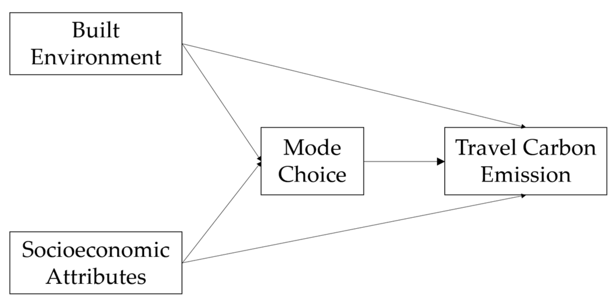
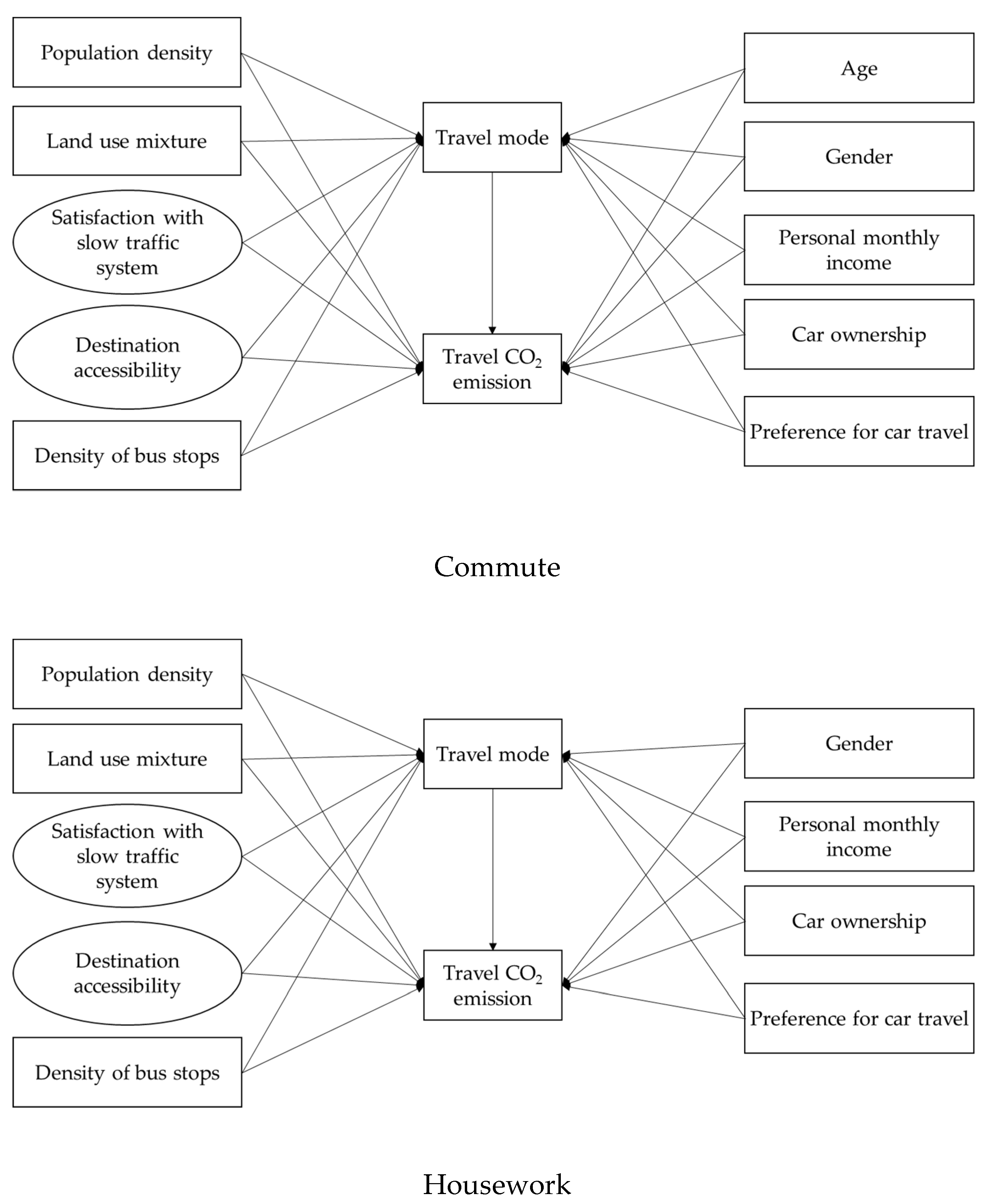
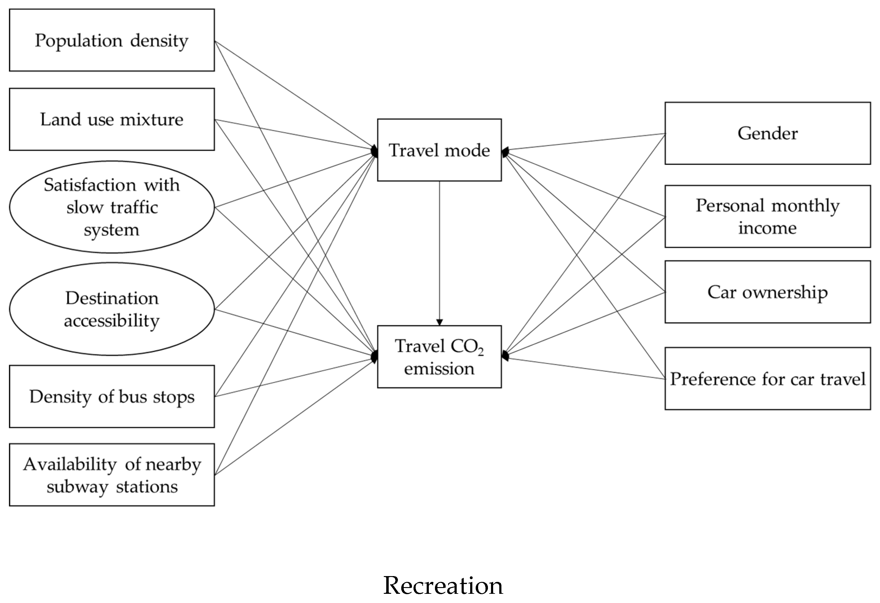
3.3. Theoretical Framework and Model

Based on the existing research, our research proposed the theoretical framework shown in Figure 6. According to the second part of this study, the built environment and personal socioeconomic attributes impact people’s travel behavior and travel carbon emissions. However, in most studies on travel carbon emissions, the analysis of travel behavior as a mediator variable is insufficient. Most research only explores the direct effect of the built environment on travel behavior or travel carbon emissions, which is not conducive to guiding urban planning and renewal. In this study, using the travel mode as a mediator and different travel purposes as subsamples, we explored the built environment’s mediating effects and direct effects on travel-related CO₂ emissions. Both the built environment and socioeconomic attributes were set as exogenous variables of the model (Figure 6). Furthermore, because the unordered categorical variable was not suitable as a mediator variable in SEM, we classified six travel modes into zero-carbon (walking, bike), medium-carbon (e-bike, bus, and subway), and high-carbon (car) travel modes. The classification was based on the carbon emission factors of each mode. Finally, the classification was brought into the model as an ordered categorical variable.

Analysis was conducted using SEM and AMOS software (version 26). SEM calculated the direct, indirect, and total effects of the built environment on travel-related CO₂ emissions. The SEM involves the measurement model, defining the linear relationship between the latent variable and observed variable, and the structural model, analyzing the causal relationship between latent variables. Since the discussion of SSTS and DA involved latent variables, the measurement model was used. The research concerns the direct, indirect, and total effects of the built environment on travel CO₂ emissions; therefore, SEM was suitable for the study. It is worth mentioning that most studies only use the observed variable to represent one aspect of built environment characteristics, while this study’s SEM sets SSTS and DA as latent variables. Each latent variable consisted of four observed variables. It was possible to discuss the impact of the built environment with multiple factors on travel carbon emissions.

4. Results and Discussion

4.1. Goodness-of-Fit for Structural Equation Models

The reliability and validity of the data were first analyzed before modeling, followed by confirmatory factor analysis (CFA) of the measurement model, and finally, adjusting the appropriate measurement model to bring it into the structural model. The Cronbach’s alpha value for the data was 0.905, which is higher than the acceptable standard of 0.7, which means the data has good reliability. The Kaiser–Meyer–Olkin (KMO) value of the data was 0.882, with a p-value of less than 0.001, indicating good data validity. In statistics, these two values are usually used to demonstrate whether the data have good validity or not [49]. We calculated them in the IBM SPSS Statistics 26.

Since the original data does not obey multivariate normal distribution, if the maximum likelihood estimation was used, it would lead to bias in the model results; therefore, the Bollen–Stine bootstrap estimation method was used in this study [18,50], and the sample size of the bootstrap was set to 1000. Based on different trip purposes, we divided the total sample into three subsamples of commutes, housework travel, and recreational travel to establish three SEM models. The model fit indices are shown in

Table 6. The model fit indices for the SEM.

Model Fit Index	Reference Value	Model 1: Commute Model	Model 2: Housework Model	Model 3: Recreation Model
Chi-square (χ2)	-	228.244	153.867	180.715
Degrees of freedom (df)	-	92	79	89
Goodness-of-Fit Index (GFI)	>0.9	0.947	0.954	0.947
Comparative Fit Index (CFI)	>0.9	0.955	0.971	0.967
Root Mean Square Error of Approximation (RMSEA)	<0.08	0.06	0.051	0.055

, with all indicators showing a good fit between the model and the sample data.

Figure 7 illustrates the path diagrams for the three models, involving variables such as the built environment of resettlement neighborhoods, travel mode, travel carbon emissions, and socioeconomic attributes. The path relationships of the three models were similar but differed in some way due to removing paths and variables that were not statistically significant, and the modified model was re-estimated in each case. This also indicates that residents’ carbon emissions from travel are influenced by different factors when travel purposes are different.

4.2. Results for SEMs

Table 7. Standardized direct and total effects of three models.

Variables	Effect	Model 1: Commute		Model 2: Housework		Model 3: Recreation
		Travel Mode	CO2	Travel Mode	CO2	Travel Mode	CO2
Population density	TE	-	-	-	-	-	−0.117 *
	DE	-	-	-	-	-	−0.104 **
	IE	-	-	-	-	-	−0.013
Land-use mixture	TE	-	-	-	-	-	−0.163 ***
	DE	-	-	-	-	-	−0.111 **
	IE	-	-	-	-	-	−0.053
Satisfaction with slow traffic system	TE	-	−0.130 ***	-	-	-	-
	DE	-	−0.090 **	-	-	-	-
	IE	-	−0.040	-	-	-	-
Destination accessibility	TE	-	−0.172 ***	−0.157 **	−0.178 ***	-	-
	DE	-	−0.118 **	−0.157 **	−0.090	-	-
	IE	-	−0.055	-	−0.088 **	-	-
Density of bus stops	TE	−0.153 ***	0.080 *	-	-	−0.325 ***	−0.325
	DE	−0.153 ***	0.169 ***	-	-	−0.325 ***	0.103 *
	IE	-	−0.089 ***	-	-	-	−0.210 ***
Subway stations nearby	TE	-	-	-	-	−0.396 ***	−0.246 ***
	DE	-	-	-	-	−0.396 ***	0.010
	IE	-	-	-	-	-	−0.257 ***
Travel mode	TE	-	0.582 ***	-	0.560 ***	-	0.648 ***
	DE	-	0.582 ***	-	0.560 ***	-	0.648 ***
	IE	-	-	-	-	-	-
Age	TE	0.102 **	0.076 **	-	-	-	-
	DE	0.102 **	0.016	-	-	-	-
	IE	-	0.060 **	-	-	-	-
Personal monthly income	TE	0.113 **	0.079 *	-	-	-	-
	DE	0.113 **	0.014	-	-	-	-
	IE	-	0.066 **	-	-	-	-
Car ownership	TE	0.160 ***	0.161 ***	-	-	0.123 **	0.148 **
	DE	0.160 ***	0.068 **	-	-	0.123 **	0.068
	IE	-	0.093 ***	-	-	-	0.080 **
Preference for car travel	TE	0.331 ***	0.263 ***	0.154 **	0.179 ***	0.171 ***	0.139 **
	DE	0.331 ***	0.070	0.154 **	0.093 *	0.171 ***	0.028
	IE	-	0.193 ***	-	0.086 **	-	0.111 ***

Note: Significance levels for direct and total effects are bootstrap approximations. Bootstrap replications = 1000. The p-value indicates significance, ‘p < 0.1’ indicates a statistical correlation between the variables, and a smaller p-value indicates a greater statistical correlation, where ‘*’, ‘**’, and ‘***’ mean ‘p < 0.1’, ‘p < 0.05’, and ‘p < 0.01’. TE is total effects; DE is direct effects; IE is indirect effects.

shows the three models’ standardized direct and total effect coefficients. Travel mode as a mediator variable in all models has a significant positive effect on travel carbon emissions.

4.2.1. Direct Effects of the Built Environment and Socioeconomic Attributes on Travel Mode

In terms of travel mode choice, a combination of the three models shows that the built environment has different significant impact factors for different travel purposes. For the commutes, the higher the density of bus stops, the lower the probability of residents choosing high-carbon (car) travel. This finding is similar to the study by Ding et al. for the Washington metropolitan area, which concluded that BSD significantly negatively impacts car ownership [51]. This implies that the more bus stops a place has, the fewer cars will be owned, and the less car travel will take place [51]. For housework travel, the significant positive impact of DA, composed of the density of daily shopping, regional shopping centers, education facilities, and sports facilities, will be on the choice of low-carbon travel mode. People who made recreational trips were more likely to be influenced by the density of bus stops (−0.325) and the subway stations nearby (−0.396), with the coefficient of the model results showing that the degree of impact of both was almost equal. In addition, population density and land-use mixture were insignificantly correlated with mode choice for all three trip purposes, with similar studies concluding that density and mixed land use have little impact on mode choice [20,52]. The increase in BSD had a higher impact on the choice of mode of recreational travel (−0.325) than commuting (−0.153). That is to say, the mode of recreational travel is more likely to be influenced by the accessibility of public transport.

For personal socioeconomic attributes, age, personal monthly income, car ownership, and preference for car travel had varying degrees of influence on people’s travel mode choice, consistent with the conclusions obtained from most studies [53,54,55]. Specifically, the older the resident and the higher the personal monthly income, the more likely the person is to choose a high-carbon commute mode. Residents who own private cars are associated with less use of low-carbon travel for both commuting and recreational. High-carbon travel is preferred for people who travel by car, not only for commuting and recreational travel, but even when undertaking housework travel.

4.2.2. Direct Effects of the Built Environment and Socioeconomic Attributes on Travel-Related CO₂ Emissions

The direct effect of the built environment on travel CO₂ varies depending on the purpose of the travel. As far as commuting is concerned, SSTS, DA, and BSD significantly impact travel-related CO₂ emissions. For SSTS, it has a significant negative effect on the carbon emissions of commuting, which means that higher SSTS around resettlement neighborhoods has a direct effect on reducing the CO₂ emissions of commutes. However, there was no significant correlation for housework and recreational trips. DA had a significant negative direct effect on the carbon emissions of commuting, which is similar to the conclusions of the research on Guangzhou and Zhengzhou [12,47]. While increased BSD can reduce the choice of high-carbon modes during a commute, it has a significant positive association with commuting carbon emissions, consistent with Yang et al.’s study of Guangzhou [18]. This suggests that reducing the high-carbon travel mode does not necessarily reduce travel CO₂ emissions. An increase in BSD may have resulted in more bus trips and more travel carbon emissions.

Housework CO₂ emissions are not statistically significant with the built environment, and only DA indirectly affects travel carbon emissions by influencing mediator variables, as will be specified in the next section.

For recreation, the impact of population density and land-use mixture on travel CO₂ emissions showed a significant negative correlation, indicating that CO₂ emissions from recreational trips are lower when the population density and land-use mixture of neighborhoods are higher. Different conclusions have been reached on the relationship between population density and travel carbon emissions. Some studies have concluded that population density has a positive effect on travel CO₂ emissions [18,33], because increased population density results in excessive travel distances. However, some research suggests a non-linear relationship between population density and travel CO₂ emissions [27]. The resettlement housing neighborhoods, generally located in the suburbs, have lower population densities than the city centers, consistent with Wu et al.’s findings [27]. Furthermore, BSD has a significant positive direct effect on carbon emissions from recreational travel (0.103), but is lower than the impact on carbon emissions from commuting (0.169).

4.2.3. Indirect and Total Effects of the Built Environment and Socioeconomic Attributes on Travel-Related CO₂ Emissions

The indirect effect of the built environment on travel-related CO₂ emissions comes from the effect of the built environment on mode choice, which in turn has a direct effect on travel CO₂. SSTS, DA, and BSD have significant indirect or total effects on travel carbon emissions in commuting. Specifically, as SSTS and DA increase, carbon emissions from commuting decrease, with standardized regression coefficients of −0.130 and −0.172 for the total effect. By influencing the choice of mode, the density of bus stops has a significant negative indirect effect on the CO₂ emissions in commuting, which is contrary to the result of its direct effect. Perhaps as the density of bus stops increases, people tend to use more public transportation rather than cars to travel; however, more carbon emissions from public transportation offset the reduction of carbon emissions from cars.

Destination accessibility showed a significant negative indirect effect (−0.088) and total effect (−0.178) with travel CO₂ emissions for housework. This shows that improving DA can reduce carbon emissions by influencing travel mode choice in housework trips.

The significant negative total effect of land-use mixture on carbon emissions from recreational travel implies that although increasing land-use mixture does not necessarily encourage low-carbon travel for all purposes, it helps to reduce CO₂ emissions from recreational travel. The influence of BSD on the carbon emissions in recreational trips shows similar results as commuting, but its influence on recreational trips is greater. Finally, nearby subway stations in residential areas can influence people’s mode choices and reduce carbon emissions from recreational trips.

5. Conclusions

Based on the travel survey data of resettlement housing neighborhoods in Nanjing, focused on the problems of spatial mismatch, excessive street scale, and inconvenient transportation, we used three-group SEM to study the impact of the built environment on the carbon emissions of three travel purposes, including commutes, housework, and recreation. By choosing the built environment variables representing the resettlement housing neighborhoods, the following conclusions and planning recommendations were proposed:

First, unlike previous similar research, we found that DA has a greater effect on the travel carbon emissions of residents in resettlement housing than the population density and land-use mixture that are commonly referred to. From another aspect, this demonstrates that the accessibility of destinations around resettlement housing remains poor. By increasing the accessibility of public services, such as daily shopping, regional shopping centers, education facilities, and sports facilities, travel distances and carbon emissions can be significantly reduced.

Second, for the resettlement housing neighborhoods in Nanjing, some built environment variables have indirect and total effects on travel carbon emissions, such as land-use mix, satisfaction with the slow traffic system and the subway stations nearby. This means that even if the built environment does not directly affect travel carbon emissions, it can indirectly affect travel-related CO₂ emissions by influencing the mediator. The mediator chosen in this study was travel mode. Similar studies have chosen car ownership and travel distance as mediators [18,33], which reinforces the existence of multiple paths of environmental influence on residents’ travel carbon emissions. Urban planners should pay attention to the long-term impact of the environment on people, such as changing people’s mode choices, reducing the purchase of cars, setting up a work-housing balance, building a non-motorized, people-oriented travel environment, and providing adequate public transportation services.

Third, differences exist in the impact paths of the built environment on residents’ travel carbon emissions for different trip purposes. SSTS, DA, and BSD influence the carbon emissions produced by commuting. Housework travel-related CO₂ emissions are only influenced by DA. Population density, land-use mix, and the subway stations nearby affect the carbon emissions of recreation. Therefore, for the planning, design, and renewal of a resettlement housing area oriented to low-carbon travel, there should be attention paid not only to commuting, but also travel for purposes such as housework and recreation, in order to comprehensively reduce CO₂ emissions.

As mentioned earlier, the suburbanization of resettlement housing neighborhoods is a common feature in China, our study can provide a case study for this phenomenon. This study has good insights into the planning, construction, and renewal of resettlement housing neighborhoods, which are generally located in the suburbs in China. Regarding the problems of spatial mismatch, excessive street scale, and inconvenient traffic in the resettlement housing areas, site selection should consider the living, working, recreation, and traffic of residents. The location choice should consider the overall cost of living, especially low-income residents. It should also ensure the distribution of resettlement houses in various parts of the city to avoid high travel costs, inadequate infrastructure, and residential segregation caused by large-scale resettlement housing construction. In the construction of resettlement housing and community renewal, it is important to consider the optimized distribution of supporting facilities and building a non-motorized travel-friendly transport environment.

In addition, the government should actively promote the advantages of low-carbon travel to residents and encourage low-carbon travel. For example, in terms of low-carbon travel awareness, people should be informed that low-carbon travel can help reduce GHG emissions and improve air quality. Additionally, low-carbon travel can increase physical activity and reduce the chance of disease. Regarding the travel mode, residents who choose a low-carbon mode will be given specific incentives to establish a low-carbon incentive mechanism. Similarly, people who frequently use public transportation will be given price discounts.

However, the study does have limitations. The calculations of travel CO₂ in this study were based on the carbon emission factors of travel modes from existing studies. There are some limitations in the values due to the differences in measurements by different researchers. Second, this research only focuses on resettlement housing neighborhoods in China’s suburbanization process; however, other types of neighborhoods exist in similar locations, and a possible future research direction would be to investigate various types of neighborhoods. Third, the impact of built environment factors on travel carbon emissions may differ for different scales, and future studies should consider built environment factors at various spatial scales.

References

1. Kinigadner, J.; Büttner, B.; Wulfhorst, G.; Vale, D. Planning for Low Carbon Mobility: Impacts of Transport Interventions and Location on Carbon-Based Accessibility. J. Transp. Geogr. 2020, 87, 102797. [Google Scholar] [CrossRef]
2. Portner, H.O.; Roberts, D.C.; Adams, H.; Adler, C.; Aldunce, P.; Ali, E.; Begum, R.A.; Betts, R.; Kerr, R.B.; Biesbroek, R. Climate Change 2022: Impacts, Adaptation and Vulnerability; IPCC: Geneva, Switzerland, 2022. [Google Scholar]
3. Zhu, Q.; Leibowicz, B.D. Vehicle Efficiency Improvements, Urban Form, and Energy Use Impacts. Cities 2020, 97, 102486. [Google Scholar] [CrossRef]
4. Perumal, A.; Timmons, D. Contextual Density and US Automotive CO2 Emissions across the Rural–Urban Continuum. Int. Reg. Sci. Rev. 2017, 40, 590–615. [Google Scholar] [CrossRef]
5. Zhang, H.; Peng, J.; Wang, R.; Zhang, J.; Yu, D. Spatial Planning Factors That Influence CO2 Emissions: A Systematic Literature Review. Urban Clim. 2021, 36, 100809. [Google Scholar] [CrossRef]
6. Acheampong, R.A. Towards Incorporating Location Choice into Integrated Land Use and Transport Planning and Policy: A Multi-Scale Analysis of Residential and Job Location Choice Behaviour. Land Use Policy 2018, 78, 397–409. [Google Scholar] [CrossRef] [Green Version]
7. Wang, S.; Liu, X.; Zhou, C.; Hu, J.; Ou, J. Examining the Impacts of Socioeconomic Factors, Urban Form, and Transportation Networks on CO2 Emissions in China’s Megacities. Appl. Energy 2017, 185, 189–200. [Google Scholar] [CrossRef]
8. Juan, Y.; Chunxiao, H. The Evolution Process and Countermeasure Research of Affordable Housing in the New Period:A Case Study of Nanjing. Mod. Urban Res. 2020, 04, 114–123. [Google Scholar]
9. Fan, L.; Cao, J.; Hu, M.; Yin, C. Exploring the Importance of Neighborhood Characteristics to and Their Nonlinear Effects on Life Satisfaction of Displaced Senior Farmers. Cities 2022, 124, 103605. [Google Scholar] [CrossRef]
10. Zhu, P.; Zhao, S.; Jiang, Y. Residential Segregation, Built Environment and Commuting Outcomes: Experience from Contemporary China. Transp. Policy 2022, 116, 269–277. [Google Scholar] [CrossRef]
11. Zhou, Y.; Ji, H.; Zhang, S.; Qian, C.; Wei, Z. Empirical Study on the Boundary Space Form of Residential Blocks Oriented toward Low-Carbon Travel. Sustainability 2019, 11, 2812. [Google Scholar] [CrossRef] [Green Version]
12. Ma, J.; Zhou, S.; Mitchell, G.; Zhang, J. CO2 Emission from Passenger Travel in Guangzhou, China: A Small Area Simulation. Appl. Geogr. 2018, 98, 121–132. [Google Scholar] [CrossRef]
13. Yang, L.; Wang, Y.; Han, S.; Liu, Y. Urban Transport Carbon Dioxide (CO2) Emissions by Commuters in Rapidly Developing Cities: The Comparative Study of Beijing and Xi’an in China. Transp. Res. Part D: Transp. Environ. 2019, 68, 65–83. [Google Scholar] [CrossRef]
14. Pérez-Neira, D.; Rodríguez-Fernández, M.P.; Hidalgo-González, C. The Greenhouse Gas Mitigation Potential of University Commuting: A Case Study of the University of León (Spain). J. Transp. Geogr. 2020, 82, 102550. [Google Scholar] [CrossRef]
15. Yang, W.; Zhou, S. Using Decision Tree Analysis to Identify the Determinants of Residents’ CO2 Emissions from Different Types of Trips: A Case Study of Guangzhou, China. J. Clean. Prod. 2020, 277, 124071. [Google Scholar] [CrossRef]
16. Wang, B.; Shao, C.; Ji, X. Influencing Mechanism Analysis of Holiday Activity-Travel Patterns on Transportation Energy Consumption and Emissions in China. Energies 2017, 10, 897. [Google Scholar] [CrossRef] [Green Version]
17. Ding, C.; Liu, C.; Zhang, Y.; Yang, J.; Wang, Y. Investigating the Impacts of Built Environment on Vehicle Miles Traveled and Energy Consumption: Differences between Commuting and Non-Commuting Trips. Cities 2017, 68, 25–36. [Google Scholar] [CrossRef]
18. Yang, W.; Cao, X. Examining the Effects of the Neighborhood Built Environment on CO2 Emissions from Different Residential Trip Purposes: A Case Study in Guangzhou, China. Cities 2018, 81, 24–34. [Google Scholar] [CrossRef]
19. Liu, Z.; Ma, J.; Chai, Y. Neighborhood-Scale Urban Form, Travel Behavior, and CO2 Emissions in Beijing: Implications for Low-Carbon Urban Planning. Urban Geogr. 2017, 38, 381–400. [Google Scholar] [CrossRef]
20. Cervero, R.; Kockelman, K. Travel Demand and the 3Ds: Density, Diversity, and Design. Transp. Res. Part D Transp. Environ. 1997, 2, 199–219. [Google Scholar] [CrossRef]
21. Ewing, R.; Cervero, R. Travel and the Built Environment. J. Am. Plan. Assoc. 2010, 76, 265–294. [Google Scholar] [CrossRef]
22. Ton, D.; Bekhor, S.; Cats, O.; Duives, D.C.; Hoogendoorn-Lanser, S.; Hoogendoorn, S.P. The Experienced Mode Choice Set and Its Determinants: Commuting Trips in the Netherlands. Transp. Res. Part A Policy Pract. 2020, 132, 744–758. [Google Scholar] [CrossRef]
23. Liu, L.; Silva, E.A.; Yang, Z. Similar Outcomes, Different Paths: Tracing the Relationship between Neighborhood-Scale Built Environment and Travel Behavior Using Activity-Based Modelling. Cities 2021, 110, 103061. [Google Scholar] [CrossRef]
24. Liu, Y.; Huang, L.; Onstein, E. How Do Age Structure and Urban Form Influence Household CO2 Emissions in Road Transport? Evidence from Municipalities in Norway in 2009, 2011 and 2013. J. Clean. Prod. 2020, 265, 121771. [Google Scholar] [CrossRef]
25. Gim, T.H.T. Analyzing the City-Level Effects of Land Use on Travel Time and CO2 Emissions: A Global Mediation Study of Travel Time. Int. J. Sustain. Transp. 2021, 16, 496–513. [Google Scholar] [CrossRef]
26. Hong, J. Non-Linear Influences of the Built Environment on Transportation Emissions: Focusing on Densities. J. Transp. Land Use 2017, 10, 229–240. [Google Scholar] [CrossRef] [Green Version]
27. Wu, X.; Tao, T.; Cao, J.; Fan, Y.; Ramaswami, A. Examining Threshold Effects of Built Environment Elements on Travel-Related Carbon-Dioxide Emissions. Transp. Res. Part D: Transp. Environ. 2019, 75, 1–12. [Google Scholar] [CrossRef]
28. Rowangould, G.M.; Tayarani, M. Effect of Bicycle Facilities on Travel Mode Choice Decisions. J. Urban Plan. Dev. 2016, 142, 04016019. [Google Scholar] [CrossRef]
29. Nakshi, P.; Debnath, A.K. Impact of Built Environment on Mode Choice to Major Destinations in Dhaka. Transp. Res. Rec. 2021, 2675, 281–296. [Google Scholar] [CrossRef]
30. Ye, R.; Titheridge, H. Satisfaction with the Commute: The Role of Travel Mode Choice, Built Environment and Attitudes. Transp. Res. Part D Transp. Environ. 2017, 52, 535–547. [Google Scholar] [CrossRef]
31. DeWeese, J.; El-Geneidy, A. How Travel Purpose Interacts with Predictors of Individual Driving Behavior in Greater Montreal. Transp. Res. Rec. 2020, 2674, 938–951. [Google Scholar] [CrossRef]
32. Næss, P. Built Environment, Causality and Travel. Transp. Rev. 2015, 35, 275–291. [Google Scholar] [CrossRef]
33. Ashik, F.R.; Rahman, M.H.; Antipova, A.; Zafri, N.M. Analyzing the Impact of the Built Environment on Commuting-Related Carbon Dioxide Emissions. Int. J. Sustain. Transp. 2022, 1–15. [Google Scholar] [CrossRef]
34. Liu, J.; Zhou, J.; Xiao, L.; Yang, L. Effects of the Built Environment on Pedestrian Communing to Work and School: The Hong Kong Case, China. Prog. Geogr. 2019, 38, 807–817. [Google Scholar]
35. Xu, Y.; Zhang, X. The Residential Resettlement in Suburbs of Chinese Cities: A Case Study of Changsha. Cities 2017, 69, 46–55. [Google Scholar] [CrossRef]
36. Guan, C.H.; Srinivasan, S.; Nielsen, C.P. Does Neighborhood Form Influence Low-Carbon Transportation in China? Transp. Res. Part D: Transp. Environ. 2019, 67, 406–420. [Google Scholar] [CrossRef]
37. Huang, Y.; Gao, L. Influence Mechanism of Commuter’s Low-Carbon Literacy on the Intention of Mode Choice: A Case Study in Shanghai, China. Int. J. Sustain. Transp. 2021, 1–13. [Google Scholar] [CrossRef]
38. Statistical Bureau of Nanjing. Statistical Yearbook of Nanjing 2021; China Statistics Press: Nanjing, China, 2021.
39. Wang, N.; Tang, G. A Review on Environmental Efficiency Evaluation of New Energy Vehicles Using Life Cycle Analysis. Sustainability 2022, 14, 3371. [Google Scholar] [CrossRef]
40. Yang, W.; Chen, H.; Wang, W. The Path and Time Efficiency of Residents’ Trips of Different Purposes with Different Travel Modes: An Empirical Study in Guangzhou, China. J. Transp. Geogr. 2020, 88, 102829. [Google Scholar] [CrossRef]
41. Sobrino, N.; Arce, R. Understanding Per-Trip Commuting CO2 Emissions: A Case Study of the Technical University of Madrid. Transp. Res. Part D Transp. Environ. 2021, 96, 102895. [Google Scholar] [CrossRef]
42. Ma, J.; Liu, Z.; Chai, Y. The Impact of Urban Form on CO2 Emission from Work and Non-Work Trips: The Case of Beijing, China. Habitat Int. 2015, 47, 1–10. [Google Scholar] [CrossRef]
43. Wallner, G.; Kriglstein, S.; Chung, E.; Kashfi, S.A. Visualisation of Trip Chaining Behaviour and Mode Choice Using Household Travel Survey Data. Public Transp. 2018, 10, 427–453. [Google Scholar] [CrossRef] [Green Version]
44. McQueen, M.; MacArthur, J.; Cherry, C. The E-Bike Potential: Estimating Regional e-Bike Impacts on Greenhouse Gas Emissions. Transp. Res. Part D: Transp. Environ. 2020, 87, 102482. [Google Scholar] [CrossRef]
45. Entwicklungsbank, K. Transport in China: Energy Consumption and Emissions of Different Transport Modes; Institute for Energy and Environmental Research (IFEU): Heidelberg, Germany, 2008. [Google Scholar]
46. Cervero, R. Land-Use Mixing and Suburban Mobility. Transp. Q. 1988, 42, 429–446. [Google Scholar]
47. Zhang, J.; Zhang, L.; Qin, Y.; Wang, X.; Zheng, Z. Impact of Residential Self-Selection on Low-Carbon Behavior: Evidence from Zhengzhou, China. Sustainability 2019, 11, 6871. [Google Scholar] [CrossRef] [Green Version]
48. Guo, Y.; Liu, Y.; Lu, S.; Chan, O.F.; Chui, C.H.K.; Lum, T.Y.S. Objective and Perceived Built Environment, Sense of Community, and Mental Wellbeing in Older Adults in Hong Kong: A Multilevel Structural Equation Study. Landsc. Urban Plan. 2021, 209, 104058. [Google Scholar] [CrossRef]
49. Chen, S.; Fan, Y.; Cao, Y.; Khattak, A. Assessing the Relative Importance of Factors Influencing Travel Happiness. Travel Behav. Soc. 2019, 16, 185–191. [Google Scholar] [CrossRef]
50. Mouratidis, K. Built Environment and Leisure Satisfaction: The Role of Commute Time, Social Interaction, and Active Travel. J. Transp. Geogr. 2019, 80, 102491. [Google Scholar] [CrossRef]
51. Ding, C.; Cao, X. How Does the Built Environment at Residential and Work Locations Affect Car Ownership? An Application of Cross-Classified Multilevel Model. J. Transp. Geogr. 2019, 75, 37–45. [Google Scholar] [CrossRef]
52. Cervero, R. Mixed Land-Uses and Commuting: Evidence from the American Housing Survey. Transp. Res. Part A Policy Pract. 1996, 30, 361–377. [Google Scholar] [CrossRef]
53. Gehrke, S.R.; Wang, L. Operationalizing the Neighborhood Effects of the Built Environment on Travel Behavior. J. Transp. Geogr. 2020, 82, 102561. [Google Scholar] [CrossRef]
54. Wu, W.; Wang, M.X.; Zhang, F. Commuting Behavior and Congestion Satisfaction: Evidence from Beijing, China. Transp. Res. Part D Transp. Environ. 2019, 67, 553–564. [Google Scholar] [CrossRef]
55. Yu, L.; Xie, B.; Chan, E.H.W. Exploring Impacts of the Built Environment on Transit Travel: Distance, Time and Mode Choice, for Urban Villages in Shenzhen, China. Transp. Res. Part E Logist. Transp. Rev. 2019, 132, 57–71. [Google Scholar] [CrossRef]
Figure 1. Study area.
Buildings 12 01718 g001
Figure 2. The distribution of surveyed neighborhoods.
Buildings 12 01718 g002
Figure 3. The distribution of samples’ travel origin, destination and travel flow.
Buildings 12 01718 g003
Figure 4. The proportion of travel modes and the average distance for the three travel purposes.
Buildings 12 01718 g004
Figure 5. ECDF curves of travel-related CO2 emissions.
Buildings 12 01718 g005
Figure 6. Theoretical framework of SEM.
Buildings 12 01718 g006
Figure 7. SEM path diagram.
Buildings 12 01718 g007aBuildings 12 01718 g007b