Unravelling the Relations between and Predictive Powers of Different Testing Variables in High Performance Concrete Experiments: The Data-Driven Analytical Methods

Zhuang, Zheng-Yun; Kuo, Wen-Ten

doi:10.3390/buildings12101545

Open AccessArticle

Unravelling the Relations between and Predictive Powers of Different Testing Variables in High Performance Concrete Experiments: The Data-Driven Analytical Methods

by

Zheng-Yun Zhuang

and

Wen-Ten Kuo

^*

Department of Civil Engineering, National Kaohsiung University of Science and Technology, Kaohsiung 807, Taiwan

^*

Author to whom correspondence should be addressed.

Buildings 2022, 12(10), 1545; https://doi.org/10.3390/buildings12101545

Submission received: 13 August 2022 / Revised: 5 September 2022 / Accepted: 20 September 2022 / Published: 27 September 2022

(This article belongs to the Special Issue Applications of (Big) Data Analysis in A/E/C)

Download

Browse Figures

Versions Notes

Abstract

:

This study proposes and applies a systematic data analysis methodology to analyse experimental data for high-performance concrete (HPC) samples with different admixtures for offshore fan foundation grouting materials uses. In contrast with other relevant research, including experimental studies, the materials physics and chemistry studies, or cementitious material portfolio determination studies, this data-driven analysis provides a deep exploration of the experimental variables associated with the test data. To offer complete and in-depth perspectives, several methods are employed for the data analyses, including correlation analysis, cosine similarity analysis, simple linear regression (SLR) modelling, and heat map and heat-based tabularised visualisations; the outcome is a proposed methodology that is easily implementable. The results from these methods are validated using a pairwise comparison approach (PCA) to avoid unnecessary interference between data variables. There are several potential contributions from this work, including insights for cohered groups of variables, techniques for double check and ‘third check’, an established ‘knowledge base’ consisting of 504 SLR predictive models with their effectiveness (significance) and prediction accuracy (data-model fitness) used in practical applications, an alternative visualisations of the results, three data transforms which can be omitted in a future analysis, and three valuable theory-linking perspectives (e.g., for the relationships between destructive and non-destructive tests with respect to the variable categories). The implication that some variables are interchangeable will make future experiments less labour intensive and time consuming for pre-project HPC material testing.

Keywords:

high performance concrete (HPC); experimental parameters; data-driven analysis; pre-project material testing; pairwise comparison analysis; correlation analysis; cosine similarity; predictive regression modelling; heat map; variable transform

1. Introduction

There are many types of experiments for testing a concrete material sample. As an example, in a study [1] involving the selection of high-performance concrete (HPC) admixtures for offshore wind farm construction, potential experiments are classified into the following three categories:

(Cat1): fresh mechanical properties,
(Cat2): hardened mechanical properties,
(Cat3): the durability measures.

In the study, slump flow and the time required to flow through a V-shaped funnel were included in (Cat 1). Compressive strength (CS), ultrasound pulse velocity (USPV), and electrical resistivity on surface (ERoS) were included in (Cat 2), while anti-sulphate capability (ASC) and rapid chloride permeability (RCP) were included in (Cat 3). These categories allowed the researchers to determine the superior admixtures that included cement, fly ash, silica fume, super plasticiser, and water for grouting before building (non-floating) wind turbines with foundations constructed in the sea. One analysis, mentioned only in the paper’s Appendix, was of particular interest because it concluded that the relationship between CS and RCP could be identified (and established) as follows:

RCP = 7966.72 + (−97.76)CS.

(1)

This equation was formulated and validated through an extensive series of exploratory data analyses in that study; further details are provided in Appendix A of this study. Figure 1 provides visualisations of the final ‘effective process’ that resulted in Equation (1) using K-means (i.e., a non-supervised machine learning approach) and simple linear regression (SLR) modelling.

However, a practical benefit of the above process has not been described in the literature: such an outcome might reduce the effort to perform sample tests because with Equation (1), one of the two experimental results (e.g., RCP) can be anticipated (e.g., by CS), thereby reducing time and effort. Nevertheless, the practical benefits of this encouraging result are still limited because it was only validated for one pair of variables. Therefore, this study seeks to answer the question: Among numerous pairs of parameters tested for the HPC samples, does any other pair exist in which one parameter can be used to predict another?

In this study, a full set of data related to the experiments is sourced, and a data-driven analysis is performed following a pairwise comparison approach (PCA). To a large extent, this study identifies all pairs of concrete sample parameters in the available datasets sourced from an HPC laboratory, providing in-depth and cross-categorical views of the relationships between each variable pair and offering scientifically grounded insights about the experimental values that can be used to anticipate others.

A systematic data analysis methodology is designed and proposed utilising numerous methods, including correlation coefficient, cosine similarity, SLR modelling, and dimensional alternation (domain transform) of the variables (before estimating the parameters of the SLR model to ensure the linearity of each established model), in addition to other supplemental methods (e.g., the heatmap visualisation technique, and viewing the results from different perspectives). Using this methodology, the analysis reveals essential information about all Cat2 and Cat3 variables, the relationship between each pair of test variables, the variable’s ability to predict other variables, and the accuracy with which the variables can predict one another. The set of information obtained from the analysis (i.e., the ‘knowledge base’) can be used to benefit researchers and practitioners.

Since every pair of variables fitted with a model with sufficient predictive power (in terms of data-model fitness and model significance or effectiveness) can be summarised from the knowledge base, the results of some tests can be anticipated by using the results of other tests (if the law allows not testing every item). This could be a significant benefit to material testers whose time is valuable, and could also indirectly help reduce the cost and complexity of construction projects.

In this paper, other discussions are presented for the insights gained, particularly for the identified pairs of variables for which the results are positive (i.e., effective information). Implications are thus drawn from several aspects of the analysis, such as selecting a proper dimensional alternation method to convert the independent variable data for the established SLR model, performing both ‘double check’ and ‘third check’ by using the cosine similarity index and the relevant statistical descriptors of SLR models for the main results in the total correlation matrix, confirming theories in the existing literature or standards (between the test variables), and revealing the truth between the different destructive and non-destructive tests. Extensive discussions are also given for the utilisation of the developed knowledge base and future applications of the proposed methodological framework, as well as the time-saving effects on making material tests in each case (if the schedule for the construction project is tight). These also associate the results with theories and practices.

Section 2 reviews the literature related to the subject (i.e., the primary research question) and the methodologies to conduct this study, as well as the main data analysis methods applied. Section 3 presents the results, and Section 4 discusses the primary positive outcomes in terms of the application of methods, the practical insights gained, and the theoretical aspects of the study. Finally, Section 5 concludes this paper.

2. Literature Review and Methods

2.1. Background of the Problem

2.1.1. Renewable Energy (RE) Planning and Wind Farm Construction

For both developing and developed economies, stable and adequate supplies of energy are mandatory. However, as world’s fossil fuel-based energy resources are limited, renewable energy (RE) has emerged as a viable solution to replace conventional electric power generation [2,3]. In addition, utilising RE is also an ‘environmentally sound’ solution for a country to meet its sustainable development goals (SDGs) [4], this is also addressed by ESG (environmental, social, governance) targets that are established for business institutions [5].

Despite disagreements over the definitions of ‘RE’, ‘green energy’, ‘sustainable energy’, and ‘clean energy’, a classification of RE that is commonly accepted refers to the type of RE resource, including solar, wind, hydropower, geothermal, biomass, marine, and others [6,7,8]. This is due to the fact that the technological aspects to exploit these types of RE resource are usually totally different, thereby leading to salient ‘watersheds’ that can be told between them.

A stream of research adopting this view of classification is related to the ‘portfolios’, either in terms of selecting the optimal investment portfolio (by a company’s decision makers) [9] or determining a country’s optimal RE portfolio (by energy planners or operators within its long-term energy policy [10]. In research related to portfolios, uncertain or risky issues are also addressed [11,12]. However, in contrast to these operational management topics, more studies focus on the technologies to exploit various aspects of RE.

As an example, the technologies to exploit wind resources usually involve aspects of EE (electrical engineering), fluid dynamics/mechanics, and construction engineering (CE). Moreover, the first step in building a wind farm is typically to construct the foundations before erecting the wind turbines. For onshore or inland turbines, it is possible for the local weather conditions to be directly utilised as engineering parameters (e.g., steel structures, concrete materials, etc.). However, for offshore turbines, regardless of their working mode (i.e., fixed or floating, depending on the water depth), underwater foundations are always required, which necessitates the well-proportioned HPC material used for grouting [13].

Constructing new wind farms is necessary for a country with unique conditions to exploit its wind resources. For offshore wind farms, in the Taiwan Strait, numerous projects have taken advantage of the very shallow waters of the ‘Taiwan Bank’ [14] and the high wind availability [15]; similar projects have been developed on the edges of the Mediterranean Sea [16,17]. For on-shore or in-land wind farms, projects have been initiated near the Sahara Desert, e.g., budget has been allocated for the construction of wind farms in Algeria [18].

The motivation of this study is to explore and better understand the parameters (or the parametric performance) of the HPC materials (the numerical values for which can be obtained experimentally) used for grouting the structural bases of offshore wind turbines. This may benefit the selection process before the real admixture of the HPC is determined and applied as grouting, and it may also generate a novel knowledge set to be used for anticipating the potential outcomes of experiments.

2.1.2. The Special Weather/Sea Conditions in Taiwan and the Effects for Wind Turbines

As discussed in several studies, the soil of Taiwan is rich in sulphates and crystalline salts due to its geological features which result from frequent crustal deformation [19,20]. Osmosis of sulphate that occurs in concrete has caused serious problems for inland structures; the gypsum reaction is one such reaction, which can inflate the concrete and peel the surface off from the structure [1]. Therefore, anti-sulphate capability is typically a critical durability parameter in this context.

In addition, the high temperature and high humidity of Taiwan may accelerate these effects and decrease the life of structures. Moreover, the frequent earthquakes in the Circum-Pacific Belt and the typhoons that originated in the West Pacific region may also cause unexpected damage to structures. The damage is ‘unexpected’ because such events usually are inherently random, as is the scale of the event, e.g., the 921 Taiwan Earthquake of 1999, the Typhoon Morakot, etc. [21,22]. These types of natural disasters should be considered to be different from the damage caused by other types of unexpected events, such as fires [23].

These same conditions also apply to the Taiwan Strait, within which the Taiwan Bank is a very large but shallow continental shelf as a potential site for constructing offshore wind farms. Despite a high availability wind field above the sea all year, the land under water is susceptible to acid attacks (such as sulphates, chlorides, etc.), experiences the same extreme climate conditions discussed above (high temperature and high humidity), suffers from frequent natural disasters (earthquakes and typhoons) [24], and is scoured by the changing ocean currents throughout the year [25]. Therefore, quality HPC material is always required for wind turbines for its good workability during grouting, its beneficial mechanical properties during construction, and its long-term durability.

Thus, the parameters of an HPC sample (i.e., the experimental values from individual tests for all HPC samples which become ‘variables’ during data analysis) should be further studied and clearly understood. In addition, a suitable method is needed to determine the optimal HPC materials for construction based on the parametric data of the samples being tested during the experiments.

The parameters included in this study are organised and shown in Figure 2. It should be noted that, unlike in previous studies, electrical resistivity on surface (ERoS) is considered to be a durability property (parameter) of HPC samples in this research. This is believed to be a more reasonable consideration based on recent studies [26,27,28].

In Figure 2, the two fresh-property parameters are excluded from this study. These two tests are usually related to the workability of an HPC material during the engineering process, and their data formats are usually incompatible because the ‘data sampling periods’ of these two experiments are different than those in the other two categories. In contrast, the other eight variables have a quite large overlap in terms of their data sampling periods, so their data formats are compatible for the analysis (see Section 3.1).

In this study, the barrier between the hardened mechanical properties and durability properties is also removed intentionally. By doing so, not only can the pairs of parameters within a certain category be explored, but so can the pairs of parameters across two categories, so that relations between them and the intensities of the relations can be identified and evaluated. As will be shown later in Section 2.3, these relations include correlations, similarities, and predictive associations in terms of the ability to use one parameter to anticipate another (and how ‘safely’ it can be used).

2.2. About the Parameters

This section provides a review and discussion of the eight testing parameters of HPC analysed in this study (see Figure 2), regardless of the barrier between the hardened mechanical and durability parametric categories (see Section 2.1.2).

2.2.1. Compressive Strength (CS)

The CS of a concrete material (sample) is defined as its ability to withstand stress without failure. In concrete design and quality control, CS is the most generally specified property. The standard test method(s) for CS is (are) defined by ASTM C39 [29].

2.2.2. Tensile Strength (TS)

In this study, the splitting tensile strength (TS) of cylindrical specimens is accepted as the main tensile TS measurement for a concrete (and HPC) material (sample). Its test(s) can be performed in accordance with ASTM C496 [30].

2.2.3. Flexural Strength (FS)

The primary property for a concrete material (sample) to demonstrate is CS, but its tensile behaviours are also important. When reinforced concrete (RC) is subjected to tensile force, cracks and expansion will occur, depending largely on the TS of the concrete material. Direct tension tests of concrete are seldom performed, mainly because the device that holds the specimen may introduce secondary stresses that introduce error in the measurement. Another test for estimating the TS of a concrete material (sample) is the ASTM C78 (third point) flexural loading test, the result of which is referred to as flexural strength (FS) in this study [31].

2.2.4. Hardness (by Rebound Hammer) (HbRH)

The rebound hammer method utilises non-destructive testing techniques to measure the concrete strength. This test can be performed in accordance with ASTM C805 [32].

2.2.5. Ultrasound Pulse Velocity (USPV)

USPV is another common non-destructive index. The structural compactness in the specimen can be estimated according to the ultrasonic transferring rate (i.e., the speed of ultrasound waves going through the sample). The more complete the hydration reaction inside the concrete, the smaller the pores will be; thus, the detected USPV increases. ASTM C597 details the method(s) to test USPV [33].

2.2.6. Anti-Sulphate Capability (ASC)

Sulphate penetrates the surface of the concrete by infiltration, and a chemical reaction is produced when it combines with calcium hydroxide in the cement; when this occurs, the concrete expands, which further peels off the surface or destroys it. The experiment to measure the anti-sulphate capability of the HPC material samples can be carried out according to ASTM C1012; this method evaluates the resistance of the HPC to sulphate attack by measuring the rate of weight loss in an immersed specimen [34].

2.2.7. Rapid Chloride (Im-)Permeability (RCP)

Another indicator of the durability of concrete is its ability to resist chloride ion penetration. This can be performed by testing the concrete material samples using a rapid chloride ion rapid test (RCPT) with an applied electrical voltage. This test method can be performed in accordance with ASTM C1202 [35].

2.2.8. Electrical Resistivity on Surface (ERoS)

To evaluate concrete compactness and the durability of cement composites in an HPC sample, the ERoS can be measured. The higher the electrical resistance, the more compact the substrate, which increases durability. This study considers ERoS to be a durability variable (see Section 2.1.2), which can be tested using ASTM C876 [36].

2.3. The Methods: A Brief Review

2.3.1. Correlation Analysis

This study uses the Pearson correlation coefficient (P-Co-Co) method as the basis of the analysis to identify the correlation between each pair of experimental parameters (variables). The computation of a P-Co-Co is typically defined as the following:

P C o C o (X, Y) = \frac{n \sum_{i}^{n} (X_{i} Y_{i}) - (\sum_{i}^{n} X_{i}) (\sum_{i}^{n} Y_{i})}{\sqrt{n \sum_{i}^{n} (X_{i}^{2}) - {(\sum_{i}^{n} X_{i})}^{2}} \sqrt{n \sum_{i}^{n} (Y_{i}^{2}) - {(\sum_{i}^{n} Y_{i})}^{2}}}

(2)

where X and Y are variables between which the P-Co-Co is to be calculated; n is the data size (length) of each variable; and i is the identifier for a specific data entry.

There are two primary reasons for using the P-Co-Co method:

(1): All of the variables are continuous, so the two variables when searching for cor-relations must also be continuous; therefore, the P-Co-Co meets the analytical purpose.
(2): Developed more than 100 years ago, P-Co-Co is the most common (and standard) method to compute and examine the correlation between two continuous variables.

2.3.2. Cosine Similarity Analysis

The cosine similarity (Cos-Sim) analysis diverges from the traditional thinking in statistics, treating experimental parameters as ‘vectors’, rather than ‘variables’; in so doing the similarity between two series of parametric values from the tests can be justified by the Cos-Sim index in the dimensional space. The standard computational process for this index can be written as:

C o s S i m (X, Y) = \frac{\sum_{i}^{n} X_{i} Y_{i}}{\sqrt{\sum_{i}^{n} X_{i}^{2}} \sqrt{\sum_{i}^{n} Y_{i}^{2}}}

(3)

where X and Y are variables being treated as vectors between which the index is to be calculated (so X_i or Y_i is the i-th element of vector X or vector Y); the other symbols are as defined previously.

The reasons to apply Cos-Sim in this context are as follows:

(1): Cos-Sim has been proven to be an effective supplemental measure to P-Co-Co in real applications [37,38];
(2): Cos-Sim also fits the data variables, i.e., the variables considered in this study are all continuous and positive, so the vectors are all meaningful in the multi-dimensional data space.

2.3.3. Simple Linear Regression

In this study, the predictive power and the relevant statistical descriptions between a pair of variables are justified by building several SLR models. Every SLR model chooses a data transform (method) to convert the independent variable (i.e., the RHS variable) prior to parameter estimation, so the model remains linear. A typical SLR model is defined as follows:

Y_{i} = α + β X_{i} + ε_{i}

(4)

where

α

and

β

are the intercept and the regression coefficient associated with the only independent variable X in the model, respectively, which are to be estimated; given the i-th data tuple in the dataset,

(X_{i}, Y_{i})

,

ε_{i}

is the residual of this data tuple with respect to

Y = α + β X

; other symbols are as defined previously.

The SLR model

Y = α + β X

can then be plotted as the best line fit (i.e., the ‘AB-line’) that includes all data points

(X_{i}, Y_{i}), \forall i \in {1, 2, \dots, n}

in the data space. This model also satisfies the requirement to identify the causal relationship and predictive power between two variables ‘pair-wisely’, i.e., the PCA used in the overall analysis (which also applies to the correlation analysis and the cosine similarity analysis).

In our analysis, every time two variables are paired, one variable becomes the dependent variable Y and the other one becomes the independent variable X. This then yields a total number of

C_{2}^{8} \times 2! = 56

‘base models’ of (X, Y), and in each case, the two paired variables are interchangeable (to appear on the RHS or LHS of the model, i.e.,

2!

).

2.3.4. Data Variable Transforms

As discussed above, each of the 56 ‘basic models’ justifies the predictive relation and power between a certain pair of variables and the relevant statistical descriptions for the SLR model. However, the models are established based on the assumption that no variable is transformed, i.e., both variables on the RHS and LHS in the model use their data values in the source domain.

In this study, we transform the values of the independent variable on the RHS of each of the 56 models in nine ways in prior and build nine models by re-estimating the parameters of the SLR model that fit the independent variable in the transform domain. For comparison purpose, the models also include the initial case of ‘no transform’ (i.e., the base model), and are written as:

(1): RHS Variable Transform: $X^{'} = X^{1}$ (no transform; the basic model)
(2): RHS Variable Transform: $X^{'} = X^{2}$ (square)
(3): RHS Variable Transform: $X^{'} = X^{3}$ (3 power)
(4): RHS Variable Transform: $X^{'} = e^{X}$ (e power X)
(5): RHS Variable Transform: $X^{'} = 2^{X}$ (2 power X)
(6): RHS Variable Transform: $X^{'} = \sqrt{X}$ (square root of X)
(7): RHS Variable Transform: $X^{'} = \sqrt[3]{X}$ (triple root of X)
(8): RHS Variable Transform: $X^{'} = \log (X)$ (log of X, base 10)
(9): RHS Variable Transform: $X^{'} = \lg (X)$ (log of X, base 2)

With all these transforms performed prior to establishing the model, the model can be simplified as Equation (5) uniformly, and the linearity for all other SLR models derived from a basic model also holds:

Y = α + β X^{'}

(5)

For a model with (X, Y) as the RHS and LHS variables, the 56 cases already included their counterpart, i.e., (Y, X) as the RHS and LHS variables, respectively (see Section 2.3.3), meaning that all cases would be considered. As such, since there are nine models derived from each ‘basic model’ totally, there would actually be 56 × 9 = 504 SLR models in this work using the same set of data.

2.3.5. Indicators Used to Justify the SLR Modelling Results

Other than P-Co-Co and Cos-Sim which are in themselves ‘indicators’ for paired data variables, in this study, the following measures are used to tell the quality of an established SLR model. These include:

(1): The estimated value of parameter $α$ , $α^{*}$ : this is the intercept of the predictive SLR model that fits the data, which is one of the two parameters defining the model in Equation (5);
(2): The estimated value of $β$ , $β^{*}$ : this is the slope of the predictive SLR model, which is another parameter that defines the model in Equation (5);
(3): The p value of the entire SLR model: this value indicates whether the model is significant or not; the significance of an SLR model usually dictates whether the model is reliable and the extent to which it can be trusted;
(4): The p value for $α^{*}$ : this p value indicates whether the estimated parameter $α^{*}$ in the SLR model is significant or not;
(5): The p value for $β^{*}$ : this p value indicates whether the estimated parameter $β^{*}$ in the SLR model is significant or not;
(6): The R-square value, $R^{2}$ : this value usually connotes the data-model fitness, i.e., how well does the obtained SLR model fit the given data of $(X_{i}, Y_{i})$ , wherein the parameters in this case are typically estimated using the OLS (ordinal least square) method; and
(7): The R-square value, ${(R^{2})}^{*}$ : this is another R-square value that is adjusted based on $R^{2}$ and the sample size; we primarily observe the traditional $R^{2}$ value in this study, since the two values are usually very similar.

To visualise the summarised and tabularised computational results, they are also plotted as heat maps to provide a clear view. A heat map is a visualisation tool that is frequently used in the field of data-driven decision-making (DDDM) since Toussaint Loua provided its first application in 1873.

3. Results

3.1. Original Datasets

The experimental datasets for the eight hardened mechanical or durability parameters, i.e., the eight variables of the HPC samples to be analysed, are summarised in Table 1. The datasets are presented following the order provided in Section 2.2.

3.2. Correlation Analysis

Table 2 shows the P-Co-Cos between each pair of variables in a correlation matrix, while no variable is transformed. Figure 3 visualises the results using a heat map.

To ensure an objective basis using the adopted measures (see Section 2.3) and taking the data variables pair-wisely, every data variable should have an equal length and be tested on the same set of testing days for the same set of HPC samples. Fortunately, the collected datasets have followed these conditions. Inside the red boxes shown in Table 1, experimental data are provided for all data variables on day 28, day 56, and day 91, over all HPC samples. The result is eight variables with an equal data length of n = 36, correspondingly; these form the basis of subsequent data analyses.

Each sub table in Table 3 shows a correlation matrix produced when variable X in each pair (of variables) is transformed using one of the methods discussed in Section 2.3.4. In these sub tables, the cells are shown in different colours to visualise the results directly (which is analogous to using a separate heat map: dark green for 1, gradient green (lighter and lighter) for (less) positive values, white for 0, gradient red (heavier and heavier) for (more) negative values, full red for −1). In addition, note that the diagonal elements are white boxes with ‘---’ entries to indicate they do not contain any meaningful information.

3.3. Cosine Similarity Analysis

Table 4 shows the Cos-Sim between each pair of variables in a matrix, with no variable transformations. Figure 4 visualises the same results using a heat map.

Some studies have successfully treated variables as vectors and used the Cos-Sim between two vectors (see Section 2.3) to confirm the correlation between two variables (but not vice versa), and have observed that a higher P-Co-Co (between −1 and 1) most often indicates a higher Cos-Sim (between 0 and 1). Since in Figure 4 most variable-pairs with higher Cos-Sim indices are observed to have higher P-Co-Cos in Figure 3 (relative to other pairs), the findings from the previous studies are confirmed in terms of P-Co-Co.

Since this outcome can provide justification for performing subsequent analyses, results were not obtained in this study for the other eight transforms. Relevant tables and figures are omitted, as those outcomes are expected to be analogous.

3.4. Regression Analysis

This section summarises the results for estimating and establishing the 504 SLR models (see Section 2.3.4). The details are summarised in the web page at the following URL: http://www.DDDM.nkust.edu.tw/download/HPCStudy2_TheUltimateDataExperiments.html (accessed on 3 April 2022) (and in Appendix B), while some initial entries in Table A1 are listed in Table 5 for clarification. A guideline for reading these tables is provided below.

In Table A1, ‘X’ determines the eight ‘main phases’ defined by the eight variables used as the independent variable. In the table, the different background colours denote these phases as blocks. In each main phase fixing the independent variable, there are seven subphases defined by other variables used as the dependent variable ‘Y’. Since each subphase involves nine transforms (refer to the transform descriptions in Section 2.3.4), each block in Table A1 contains 7 × 9 = 63 SLR models, giving 63 × 8 = 504 models in total.

For each model, M# represents the unique model number assigned, with the P-Co-Co between the independent and dependent variables (X and Y) given. This is followed by the estimated model parameters:

α^{*}

(the estimated value of parameter

α

) and

β^{*}

(The estimated value of

β

); the p values for

α^{*}

,

β^{*}

the entire SLR model,

p (α^{*})

and

p (β^{*})

; and the R square values,

R^{2}

and

{(R^{2})}^{*}

.

As an example, the model with M# = 10 in Table 5 is the model established in the main phase ‘X = CS’ and in the subphase ‘Y = FS’ to identify the relationship between CS and FS of the HPC samples. Since it is the first model of the ‘X = CS, Y = FS’ subphase, transform method (1):

X^{'} = X^{1}

is used, which means no transform is performed for the data of variable X in this model (see Section 2.3.4). From the table, the estimated parameters for this model are:

α^{*}

= 4.243931 (meaning the regression line intercepts with the Y axis at Y = 4.243931) and

β^{*}

= 0.104528 (this is the regression line’s slope, meaning one unit of increase in CS leads to an increase of 0.104528 in FS). Therefore, the established model can be written as:

F S = 4.243931 + 0.104528 \times C S

(6)

For the same model, p(

α^{*}

) = p(

β^{*}

) = p(M) = 0. Despite the fact that in this table the p values are truncated to 4 digits past the decimal so that ‘p = 0′ may represent a very small value of p, it could still be inferred that both parameters estimated by the model are very significant, and the model itself is quite significant (i.e., it is very reliable and can be trusted to a large extent).

Moreover, for this model,

R^{2}

= 0.679376 and

{(R^{2})}^{*}

= 0.669946, meaning that the data-model fitness is acceptable, since over 2/3 of the variability is explained by the established model. However, this is only slightly above the acceptability threshold of 0.6 to claim data-model fitness which was established due to this study’s scientific foundation (i.e., natural science than social science investigation, so using 0.6 than 0.4 or even 0.2 is more reasonable).

The full forms of all 504 models are provided in Table A2, which can also be accessed on the web page. For example, Equation (6) for the model with M# = 10 above is the same full form as displayed in Table A2.

3.5. Additional Information

Additional information about the SLR models is retrieved from Table A1 and rendered in terms of the transform method used to convert the data value of the independent variable, X. For the analytical targets, only the p and

R^{2}

values for all models are considered to conserve space. The reason for considering these values is that the p value of any regression model represents its significance, and

R^{2}

indicates the data-model fitness (or the model’s explanation power for the variations in the data), both of which are essential for qualifying SLR models.

The results for the p values of the entire model are listed in Table 6. Each sub table contains all pairs of variables (X, Y); X and Y are the RHS (independent) and LHS (dependent) variables in Equation (5), respectively. In the sub tables, the rows are identified by X and the columns are identified by Y. The significant results, indicating the SLR model is reliable and the model’s predictive power can be trusted, are shown in red font. The significance of the p values is determined using the threshold: p < 0.10, which is typically the most relaxed condition that is acceptable by statisticians. In addition, ‘p = 0′ may mean a very small value of p.

The results for the

R^{2}

values of the entire model are listed in Table 7, where each sub table contains the

R^{2}

values for the SLR models of all pairs of variables (X, Y) when a transform is applied for X. Similar to Table 6, the rows are identified by X and the columns are identified by Y in Table 7. However, unlike the correlation values which may range from −1 to 1 in Table 3, the R-squared values only range from 0 to 1. Therefore, the numbers in Table 7 are dyed according to the following convention: dark green for 1, gradient green (lighter and lighter) for (less) positive values, and white for 0.

To conserve space, the results of importance are shown with different shades of background colours in the table. In this manner, the SLR models with better data-model fitness can be easily identified. To evaluate the fitness, many scientific studies use the threshold: >0.4 (i.e., it has resolved more variations in the data, so using this model for prediction is therefore more accurate). The results for other observations, such as the p values of the estimated parameters

α^{*}

and

β^{*}

, as well as the adjusted

R^{2}

value for the model, are summarised in Table A3, Table A4 and Table A5, respectively, in Appendix C. These may also be accessed on the ‘web page’.

4. Insights and Discussions

By analysing the results, many interesting insights can be gained. For the purpose of this study, only the most critical insights are discussed in this section; other advanced information may be obtained from the detailed results in the appendices.

4.1. For Method Applications

4.1.1. Insights for Data Pre-Processing Results

During data curation and pre-processing (see Section 3.1), the fresh properties of HPC are excluded because of data incompatibility, and only the hardened mechanical and durability property data at day 28, day 56 and day 91 are utilised for analysis due to data commonalities (i.e., they provide equal-sized data variables and have overlaps in testing time), despite the fact that the frequency of data recording for the experiment is typically predefined [39]. This experience will be useful for locating commensurable HPC testing data during any future analysis.

4.1.2. Insights for Correlation Analysis Results

In the correlation analysis (see Section 3.2), the main results in Table 2 and Figure 3 reveal that:

There are two strongly correlated groups of variables: {CS, TS, FS} form a salient group, while {ASC, RCP} form another. All of the correlations identified are either very strong (r > 0.8) or near very strong (0.6 < r < 0.8 but r~0.8).
Each group in 1. exists with respect to the same variable category, i.e., CS, TS and FS are hardened mechanical properties, and ASC (in terms of the weight loss percentage) and RCP (in terms of the coulombs measured) are both durability properties.
TS is a variable of interest because it forms a medium correlation group with USPV and ERoS. It has a strong (0.6 < 0.622967 < 0.8) positive correlation with USPV and a medium (0.4 < 0.562644 < 0.6) correlation with ERoS. Since USPV also has a strong positive correlation with ERoS (0.645174), {TS, USPV, ERoS} is another correlated group that overlaps both parametric categories of an HPC sample.
The observation of negative correlations is of interest, but there are no strong or very strong negative correlations (<−0.6) identified among all variables.
USPV has similar medium negative correlations with both ASC (−0.56893) and RCP (−0.58283); this can be explained by the fact that ASC and RCP are strongly correlated (0.817532).
ERoS and ASC have a medium negative correlation (−0.54312), and TS and HbRH have a medium (but near-weak) negative correlation (−0.40234). Since a negative correlation does not actually mean a ‘poor relation’ but rather a relation in the opposite ‘direction’, the observations of the above medium-negative P-Co-Cos are meaningful.

Beyond the correlations, additional information is provided. Table 3 includes eight sub tables with correlations produced when variable X (of the variable pair (X, Y)) is converted using the eight transformation methods described in Section 2.3.4. These sub tables confirm the main results in Figure 3 and Table 2 (when no data variable is transformed), and also help identify the optimal transforms to be used for each variable (this is further discussed in Section 4.1.4). In this regard, such information is valuable.

4.1.3. Insights from the Results of the Cosine-Similarity Analysis

By treating the data variables as vectors, the results obtained from the cosine-similarity analysis essentially confirm the correlations identified between pairs of variables. With few exceptions, a higher Cos-Sim index (between 0 and 1) in Table 4 indicates it has also had a relatively high P-Co-Co in Table 2 (between −1 and 1); this result can also be observed by comparing Figure 3 and Figure 4. As such, the main results of the correlation analysis are further confirmed (and ‘double checked’, in addition to the confirmations provided in Section 4.1.2 by the P-Co-Cos recalculated after different variable transforms).

Another insight of this research relates to methodology and theory. This study offers new support for the claim that a cosine-similarity analysis can be used as a supplement to the traditional correlation analysis.

4.1.4. Insights from the Established SLR Models

In this study, after successfully estimating the model parameters used in the datasets, 504 SLR models are established. The major insights gained from these analyses are summarised as follows.

The Established ‘Knowledge Base’ Is Novel and Benefits Future HPC Sample Testing

The information relating to the established models (see Table A1 and Table A2) is valuable because it can be used to create a true ‘knowledge base’ for practical applications. Given this knowledge base, if one experimental variable for the HPC sample can be used to predict another variable based on the known mathematical relationship and a guarantee of prediction accuracy, it is logical that the number of testing items that are truly necessary may be reduced. This is particularly true today as stakeholders in the construction and civil engineering industries have reduced the time and resources needed to complete a project, so the time available to test the HPC samples is limited. This should be considered as the primary and original contribution of this study.

A Method Is Provided to Explore the Insights into the Variables That Can Practically Be Used to Predict Another Variable and to Determine How Accurate the Prediction Will Be

Table A1 lists nine SLR models (where eight other models are derived from the first ‘base model’) as a group. It is critical for data analysis in such a design to utilise all opportunities to identify the optimal model that offers both better predictive power and better data-model fitness simultaneously.

Examining SLR models in which variable X is CS, for example (M# = {1, 2, 3, …, 27} in Table 5), the first nine models are established for predicting TS (Y) from CS (X). If p(M) < 0.5 is the threshold to confirm a model’s significance, the M# = 4 (

X^{'} = e^{X}

) and M# = 5 (

X^{'} = 2^{X}

) models are not qualified to be effective (p(M) = 0.0558 and p(M) = 0.0540). In addition, the models are far from data-model fitness, because

R^{2}

= 0.103447 for M# = 4 and

R^{2}

= 0.104875 for M# = 5 (which are far below the levels of data-model fitness for seven other models), meaning that these two models may not provide good prediction accuracy. Based on these two results, it is evident that the two SLR models with the 2 ‘power X’ transforms are inadequate. A negative implication of this finding could be that the true relation between CS and TS does not exist on this basis, but a positive implication could be that there have been seven models that can be recommended (M# = {1, 2, 3, 6, 7, 8, 9}) in practice or for future research.

Investigating two subsequent (X, Y) combinations, for M# = {10, 11, …, 18}, the models are established for predicting FS (Y) from CS (X). The resulting situation is similar to using CS to predict TS: the two ‘power X’ SLR models (M# = {13, 14}) are inadequate, and “no true relation between CS and FS exists on this basis”. However, the claim can also be made that “another 7 models (M# = {10, 11, 12, 15, 16, 17, 18}) can be effective in practice or for future research”.

The M# = {19, 20, …, 27} are also established for predicting USPV (Y) from CS (X). However, no model is qualified to build a predictive relation between these two variables. Two SLR models (M# = {22, 23}) are ineffective (p > 0.1), and every model’s

R^{2}

value is poor (

R^{2}

< 0.2) meaning they provide insufficient data-model fitness. Thus, we conclude that that the value of USPV from the value of CS in the experiments performed to test HPC samples cannot be anticipated, and that further research is recommended to find a method to predict USPV using CS.

This analysis is not continued throughout the entire Table A1. The above process can be repeated for all other models in Table A1 to gain other insights regarding the variables that can be used to predict other variables and the accuracy of the prediction process. In addition to these empirical insights that are expected, the experimental design to enable such explorations is the second contribution of this work.

Another Perspective to View the Model Information Is Offered to Differentiate and Recommend the Appropriate Transforms to Be Used for a Variable

An alternative method to evaluate the information relating to the established SLR models can provide additional insights. In Section 3.5 and Appendix C, the significance of the entire model (p(M)), the significance of the estimated

α^{*}

value (i.e., p(

α^{*}

)), the significance of the estimated

β^{*}

value (i.e., p(

β^{*}

)), the R square value (i.e.,

R^{2}

), and the adjusted R square value (i.e.,

{(R^{2})}^{*}

) of the SLR models are systematically presented as separate tables (Table 6, Table 7, Table A1 and Table A2) according to the transform applied on the RHS variable in the SLR model. This provides another perspective for the model information which can be used in addition to the previous analytical viewpoint that presents a group of models derived from a base model at the same time (e.g., Table 5, Table A1 and Table A2). Therefore, offering two complementary perspectives is another contribution of this research. The following discussion highlights the positive outcomes of this new data-viewing perspective.

Based on the results in Table 6 and Table 7 (for the p(M) values and the

R^{2}

values, respectively), the following insights are gained:

7.: In most of the RHS variable transformation cases (refer to the corresponding sub tables in Table 6), the SLR model’s p(M) value agrees with that of the ‘no transform’ case (shown in the ‘significant’ cells with red borders). This not only confirms that the ‘no transform’ SLR model is effective in its predictive power, but also identifies an alternative set of effective transformed SLR models.
8.: In most of the RHS variable transformation cases (refer to the corresponding sub tables in Table 7), the SLR model’s $R^{2}$ value agrees with that of the ‘no transform’ case (see the colour intensity of a cell). This not only confirms that the ‘no transform’ SLR model is able to provide accurate predictions, but also identifies an alternative set of qualified ‘having transform’ SLR models.
9.: For most of the RHS variable transforms, the SLR model’s $R^{2}$ value in Table 7 also concurs with the correlation identified in Figure 3 in terms of the equal P-Co-Co value for (X, Y) or (Y, X), and also for the counterpart model with Y and X exchanged as the RHS and LHS variables of the SLR model. In addition, the SLR model’s $R^{2}$ may also concur with the Cos-Sim index calculated for (X, Y) (and (Y, X)). In other words, if a high correlation is identified between two variables, a high data-model fitness typically exists, and vice versa. Furthermore, in such cases with high correlation and high data-model fitness, the Cos-Sim values are generally also high. These insights are critical because the relationships between these three values (P-Co-Co, Cos-Sim and $R^{2}$ ) that were previously unidentified have now been clarified for this application.
10.: The ‘lowest-performing RHS variable transforms’ can also be identified from the results, supporting the claim that the true relationship between the two variables in an SLR model (i.e., Y and the X being converted using a worse transform) is far from ‘a variable is transformed like that’. This claim further implies that some variable transformation methods can be ignored in the future.

Regarding the ‘worse variable transforms’, they can be identified by interpreting Table 6 in detail (in addition to Table A1 and Table A2, as required) to determine if, for a pair of (X, Y), a ‘no transform’ model shows good results (e.g., p(M) < 0.05 and/or

R^{2}

> 0.6), and which model(s) with a variable transform shows poor results (e.g., p(M) > 0.1 and/or

R^{2}

< 0.2)?

Examining the highly-correlated variable group of {CS, TS, FS} (see Section 4.1.2), the SLR models established between all pairs of these variables using every other transform (for X) offers a preferred data-model fitness for providing accurate predictions (i.e.,

R^{2}

≥ 0.6) (shown in the dark cells in the upper left of Table 7a,b,e–h); however, this is not the case using the two ‘power X methods’ (i.e.,

X^{'} = e^{X}

and

X^{'} = 2^{X}

) (shown in the light cells in the upper left part of Table 7c,d).

Further evaluating Table 7 reveals that for all pairs of variables, using these two ‘power X’ methods may depress the

R^{2}

value in general and make it difficult to uncover the relevant information (e.g., to determine which model provides better data-model fitness). It is therefore recommended to neglect both ‘power X’ methods in future studies for all pairs of test variables.

4.1.5. Other Insights from the Research

In addition to the above insights, several other interesting findings are obtained from the data analysis in this study.

For example, the p(M) values in Table 6g,h are identical, as are the

R^{2}

values in Table 7g,h; interestingly, the associated P-Co-Co values in Table 3g,h are also identical. By further inspecting Table 5 and A1, these can be explained by the fact that the SLR models will be identical if the transformation method is

X^{'} = \log (X)

or

X^{'} = \lg (X)

. That means that the base (here, 10 or 2) does not change if a logarithm is used for the RHS variable transform. Therefore, it is recommended for future studies that, for each pair of variables, keeping either SLR model is sufficient.

4.2. Theory-Linking

In this section, from three theoretical perspectives, the importance of several theory-reflexive finding and insights are discussed.

Through the numerical analysis, the relationship between FS and CS identified in this study (in its mathematical form) is found to concur with their relationship as defined in ACI 318-19 [40,41,42] and in [43] (except for the coefficients). Therefore, this result is reflexive to the existing theories; in turn, this outcome further validates the results obtained in this study.

Next to this, the measures, data variables, and tests established for the durability of concrete are critical, as durability is an important category of parameters for HPC, particularly when it is to be used in humid areas or marine environments which are prone to acid attacks [44,45,46]. However, due to the time required to obtain results, true tests for durability are difficult to perform, so other indirect tools such as ASC, RCP, and ERoS should be applied. For this, a conventional theory is that, if a correlation between a hardened mechanical (i.e., strength) property and another durability property can be identified (or if their causal relationship can be established), durability can thus be anticipated by strength properties. In this research, other than very strong or strong relationships identified for the HPC parameters in the same variable category, some significant relationships (from strong to median intensities) between variables across the two categories (see Section 3 and Section 4.1) are also found. In other words, these positive outcomes have confirmed the core theoretical logic.

Following these, another theoretical perspective relates to destructive and non-destructive tests (NDTs) [23,47]. Referring to Table 8, which is a simplified version of Table 2 with colour levels added (full red for 1, gradient red (lighter and lighter) for (less) positive values, gradient blue (heavier and heavier) for (more) negative values, dark blue for −1), the upper left cells containing the hardened mechanical properties show that, other than the very strong or near very strong correlations identified among the three destructive ‘strength’ measures, {CS, TS, FS}, USPV and HbRH are NDTs. Two interesting and important observations about these NDTs can be made.

The first observation is that USPV is an NDT that is more correlated with all destructive tests than HbRH, as evidenced by the magnitude of the P-Co-Cos,

|0.43176| > |- 0.39808|

,

|0.62297| > |- 0.40234|

, and

|0.31071| > |- 0.30525|

. Thus, USPV has a medium correlation with TS, a medium correlation with CS, and a weak correlation with FS, while HbRH has a weak negative correlation with TS, a weak negative correlation with CS, and a weak negative correlation with FS. Therefore, the test results for USPV may be more associated with the results obtained from the destructive tests than that of HbRH. This supports the recommendation to keep only one NDT (i.e., USPV, because it provides links to destructive tests more effectively), which is similar to the previous finding supporting the recommendation to keep only one destructive test (i.e., either CS, or TS, or FS, because they are interchangeable; see Section 4.1).

The second observation is that there is no significant correlation between the two NDTs for hardened mechanical properties, despite the fact that the test results for USPV may have a weak negative correlation with those of HbRH (−0.23428). This means that, for two similar HPC samples (with the same admixture) tested on the same day, these two NDTs would typically produce diversified results. An evidence-based argument can be presented that the mechanisms behind these two NDTs should be intrinsically different.

Similar observations to the destructive tests and NDTs can also be made by examining the lower right cells with respect to the durability properties. Other theory-reflexive insights of interest based on these results could be gained through future studies.

5. Conclusions

This study proposes and applies a systematic data analytic methodology to analyse the experimental data obtained from tests of HPC samples with different admixtures. In contrast with other relevant studies aimed primarily at performing experiments (and providing rationale for the experiments based on materials, physics, or chemistry) or identifying the optimal HPC admixture(s) for grouting concrete materials to be used in the sea (e.g., for the base construction of offshore wind turbines), the purpose of this study is to perform a thorough investigation of the experimental variables related to the testing data.

To achieve this purpose, a methodological framework is proposed. In order to generate comprehensive and in-depth views of the data, numerous methods are utilised, including P-Co-Co, Cos-Sim, SLR, and heatmap or heat-based tabularised visualisation. This approach is significantly different from those of other experimental-based research or admixture-selection studies. Highlights of the research activities, results, and insights gained are presented below.

All variables in the dataset testing the 12 HPC samples of different admixtures were previewed. The dataset was sourced intentionally to cover as many tests for HPC as possible. Among the Cat2 and Cat3 properties, the overlapping (and compatible) data for the eight variables (i.e., the data gathered at 28, 56, and 91 days for CS, TS, FS, USPV, HbRH, ERoS, ASC, and RCP) are identified and specified to support subsequent analyses.
Rather than providing a descriptive analysis for the testing data, the investigation began with a correlation analysis, in which the concept of PCA was applied. Within the same variable category, variable groups were identified in which the correlation between each pair of variables was very strong {CS, TS, FS} and {ASC, RCP}. Another medium-correlation variable group was {TS, USPV, ERoS}, in which the included variables overlap the two variable categories. In addition to the positive correlations, some relatively strong negative correlations were also identified between some pairs of variables. The result for P-Co-Cos in the main correlation matrix with no variable transformation was confirmed by another eight correlation matrices with variable X in Equation (2) being converted using transforms (2)–(9) described in Section 2.3.4.
The correlation matrix was validated using the cosine similarity analysis. With few exceptions, a higher Cos-Sim index (between 0 and 1) meant it also had a relatively high P-Co-Co.
This analysis generated 504 SLR models, establishing a novel ‘knowledge base’ which can benefit future HPC sample-testing. By grouping these models using the $C_{2}^{8} \times 2!$ = 56 ‘base models’, each group consisted of nine models (associated with the nine types of RHS variable transform, including ‘no transform’) (see Table 5). When they are grouped using the 9 types of RHS variable transform, each stratification has 56 models. These two perspectives enabled different types of subsequent analyse.
With the established knowledge base, an investigation was performed to determine if a variable can be used to predict another (or not) and, if so, how accurate the prediction will be. For example, by inspecting each SLR model’s significance value, p(M), it was shown that CS test data can safely be used to predict TS and FS for an HPC sample, but it may not be used to anticipate USPV (see Section 4.1.4). By inspecting the SLR models’ $R^{2}$ values, CS was found to predict TS and FS accurately. These results were cross-validated with the very strong correlations observed among {CS, TS, TS} from the correlation analysis. Insights such as these implied that in future construction projects, valuable time and effort can be saved with respect to HPC testing.
By utilising a second perspective to view the model information (see #4 above), the appropriate RHS variable transforms in this analytical context were identified. It was also found that the two ‘power X’ transforms (i.e., $X^{'} = e^{X}$ and $X^{'} = 2^{X}$ ) are both inadequate and should be omitted, and one of the ‘logarithm’ transforms (i.e., $X^{'} = \log (X)$ or $X^{'} = \lg (X)$ ) is redundant. Thus, at least three out of the nine transforms can be excluded in future analyses.
Some of the insights gained from the results were linked to theories, including the following: (1) The results confirmed relationships found in the existing literature or standards between the test variables; (2) The results verified that the core theoretical logic of this research is effective; (3) The results of some NDTs were more related to the destructive tests (while some NDTs were less related), and different NDTs led to different results; unlike the destructive tests (particularly strength tests), these NDTs are not interchangeable.

The methods used in this study are common, and utilising them for this study was proven to be effective. Therefore, it should also be valid to utilise the methodological framework proposed in this research for similar purposes, e.g., data analysis for other concrete samples with different admixtures. From this perspective, a future story upon taking the proposed framework is perhaps clear from scratch. When a construction project is launched, one first sees if the HPC material(s) is to be used.

As can be expected, if so (using HPC) and if the planned admixtures of the HPC samples to be tested are analogous to the ones being tested in this study, efforts related to testing the materials can be reduced considerably by either policy. The first policy is to use the direct testing results for the samples in the established knowledge base (if ‘no testing’ is allowed legally). The second is to determine the testing item to be ‘predicted’ (as desired), look up the knowledge base to know what any other testing item can predict it (and also the information about whether the prediction will be effective and/or accurate), and decide whether to really but safely save the money, and time in most of the cases, for making tests by anticipating the results for the testing item (if some regulated testing items are mandatory).

However, if so (using HPC) and the planned HPC samples to be tested are different (e.g., due to a diversified purpose of use), or if not so (using the non-HPC material), theoretically, the first step is to make similar tests for these samples, followed by using the proposed framework to conduct the thorough data experiments (in order to identify the relationship and the mutual predictive power between each pair of sample parameters). Then as can be imagined, another knowledge base for the samples included by this purpose of use can be established. Although the outcomes and the unanticipated insights gained may vary in different cases or contexts, after this one-time job, what follows is a similar policy-making problem (see the former paragraph). Anyhow, all this may support efforts to save the time required for pre-project experiments, especially when the project is urgent, which is a crucial but inevitable fact in the current A/E/C industry.

It should be noted that the applications of this framework are not limited to cases in which the source datasets for each measure are tested using conventional methods (i.e., a parameter of HPC samples may have more than one testing method). For example, the framework could be applied when a part of the data is obtained using NMR (nuclear magnetic resonance) [48,49]. In many countries, NMR equipment is legal and commercialised, and the data for some variables can be obtained [50,51]. Other than this, except for HPC, the question of ‘can similar data analysis using this framework be carried out for other construction materials?’ is also worth of exploration.

Future research directions are shown in Figure 5, wherein the aim of this study which is clearly differentiated from other relevant studies.

In the figure, the experimental-oriented studies are focused on the performance of the HPC, the inclusion of parameters for developing experiments, and statistics and variability in the data. A critical element that future research directions rely upon is the testing data sets produced by this research. Following this step, there are clear boundaries among the three research directions. The materials, physics and chemistry studies research direction involves a significant amount of opportunity for future studies. However, the knowledge base constructed for the HPC testing parameters as an outcome of the data analytics studies may benefit advance data studies in the future as well as subsequent selection decision modelling studies and current cementitious material portfolio determination studies. The selection decision modelling studies aim to rank the HPC samples with different admixtures and select the optimal candidate using the scientific decision models; therefore, the knowledge base may provide a precise numerical foundation for these models (and added value from the expert knowledge of the researchers).

Author Contributions

Conceptualization, methodology, software, visualization, Z.-Y.Z.; data curation, investigation, supervision, validation, W.-T.K.; funding acquisition, project administration, writing—original draft preparation, writing—review and editing, Z.-Y.Z. and W.-T.K. All authors have read and agreed to the published version of the manuscript.

Funding

This research was funded by Ministry of Science and Technology (MOST, Taiwan, ROC), grant number MOST 110-2410-H-992-020 and 110-2637-E-992-001. The APC was funded by MDPI discount voucher and MOST 111-2410-H-992-011. Note that the institution ‘Ministry of Science and Technology (MOST)’ has been renamed as National Science and Technology Council (NSTC) in August 2022 in this area. However, we still keep the original funding number for these projects were approved before the transition.

Data Availability Statement

N/A. All related data for the results of this study are detailed in the appendix sections.

Conflicts of Interest

The authors declare no conflict of interest.

Acronyms (Alphabetic Order)

ACI	American Concrete Institute
A/E/C	Architect/Engineering/Construction
ASC	Anti-Sulphate Capability
ASTM	American Society for Testing and Materials
Cat1	(Property) Category 1 (Fresh Mechanical)
Cat2	(Property) Category 1 (Hardened Mechanical)
Cat3	(Property) Category 3 (Durability)
CE	Construction Engineering
Cos-Sim	Cosine Similarity
CS	Compressive Strength
DDDM	Data-Driven Decision-Making
EE	Electrical Engineering
ERoS	Electricity Resistivity on Surface
ESG	Environmental, Social, Governance
FS	Flexural Strength
HbRH	Hardness by Rebound Hammer
HPC	High Performance Concrete
LHS	Left-Hand Side
NDT	Non-Destructive Test
NMR	Nuclear Magnetic Resonance
OLS	Ordinal Least Square
PCA	Pairwise Comparison Approach
P-Co-Co	Pearson Correlation Coefficient
RC	Reinforced Concrete
RCP	Rapid Chloride Permeability
RCPT	Rapid Chloride Permeability Test
RE	Renewable Energy
RHS	Right-Hand Side
SDG	Sustainable Development Goals
SLR	Simple Linear Regression
TS	Tensile Strength
USPV	Ultrasound Pulse Velocity

Appendix A

In that previous study, the data analytical process to obtain Equation (1) progressed as follows:

Each pair of (CS, ACP) data (i.e., ACP stands for accumulated charge passed for RCP) was treated as a data point (entry), considering the three testing time points (in terms of #days = 28, 56 and 91) and the 12 mixture portfolios of the concrete sample all together. This yields a data table of two variables, containing the 36 data points.
A rough trend was observed by plotting the data points (see Figure 1a; the data are sourced and replotted from the Appendix of (Kuo and Zhuang, 2021)). However, establishing a simple linear regression (SLR) model to fit them, the model did not provide a satisfactory explanation for the relationship between CS and RCP, i.e., the p value of the F statistic was acceptable but relatively week (p = 0.06415), and the regression coefficient of the SLR model was merely R² = 0.09721, which is poor. Therefore, more solid clues about the relationship must be sought for.
The approach of ‘dimensional alternation of the variables’ was performed. The square root, square and log of the predictor variable (CS) was used as new variables, so several SLR models taking one of these predicting variables and keeping the variable being predicted (accumulated charge passed, or ACP) were reconstructed. In this process, outlier removals were also considered. However, as the case using the original data of variable CS, these trials did not give any more model that is satisfactory.
The second approach of ‘finding a condensed set of data points and estimating a new SLR model that fits these data points’ was then used. It used the K-means to cluster the data points (see Figure 1b), so the cluster centres form a condensed dataset. This process, in itself, removed the outliers to a certain extent, while keeping only the representative information of the data. Eventually, an effective SLR model: “ACP = 7966.72 + (−97.76)CS” was established.
The model in (4) was effective because the R² (regression for data-model fitness) of the model was as high as R² = 0.8386. The p value of the model also showed a qualified but weak result, which was p = 0.07071. However, since this was a model with one dependent variable and only one independent variable, a further scrutiny revealed that the correlation coefficient between these two data variables was as low as r = −0.9293, which could be justified as near totally negatively correlated.

From the above experiment, the last SLR model in step (5) can serve as an accurate (or, accurately calibrated) predictor when one knows a concrete sample’s CS value and would like to postulate the value of ACP that connotes the RCP of the sample. As CS is usually treated as a ‘hardened mechanical property’ but RCPT is usually a ‘durability property’ for the high-performance concrete (HPC) materials, and as this process has revealed a relationship between two experimental variables from two parametric categories, such a predictive model should be worthy of note.

Appendix B

The information in Table A1 is associated the 504 established SLR models. Table A2 lists these models in detail.

Table A1. Results from Estimating and Establishing the 504 SLR Models.

M#	Y	X	P-Co-Co	$α^{*}$	$β^{*}$	$p (α^{*})$	$p (β^{*})$	p(M)	$R^{2}$	${(R^{2})}^{*}$
1	TS	CS	0.875333	−3.667713	0.278209	0.0466	0.0000	0.0000	0.766208	0.759331
2	TS	CS	0.858867	5.766322	0.001985	0.0000	0.0000	0.0000	0.737652	0.729936
3	TS	CS	0.835226	8.989167	0.000018	0.0000	0.0000	0.0000	0.697602	0.688708
4	TS	CS	0.321631	14.568831	0.000000	0.0000	0.0558	0.0558	0.103447	0.077077
5	TS	CS	0.323844	14.565644	0.000000	0.0000	0.0540	0.0540	0.104875	0.078548
6	TS	CS	0.880394	−22.324474	4.575331	0.0000	0.0000	0.0000	0.775094	0.768479
7	TS	CS	0.881580	−40.931240	13.814583	0.0000	0.0000	0.0000	0.777183	0.770630
8	TS	CS	0.883184	−62.850941	42.785409	0.0000	0.0000	0.0000	0.780015	0.773545
9	TS	CS	0.883184	−62.850941	12.879692	0.0000	0.0000	0.0000	0.780015	0.773545
10	FS	CS	0.824243	4.243931	0.104528	0.0000	0.0000	0.0000	0.679376	0.669946
11	FS	CS	0.816058	7.757808	0.000752	0.0000	0.0000	0.0000	0.665950	0.656125
12	FS	CS	0.799660	8.962874	0.000007	0.0000	0.0000	0.0000	0.639457	0.628852
13	FS	CS	0.336406	11.087036	0.000000	0.0000	0.0448	0.0448	0.113169	0.087086
14	FS	CS	0.337948	11.085907	0.000000	0.0000	0.0438	0.0438	0.114209	0.088156
15	FS	CS	0.824872	−2.696166	1.710449	0.1088	0.0000	0.0000	0.680414	0.671015
16	FS	CS	0.824551	−9.616035	5.155510	0.0004	0.0000	0.0000	0.679884	0.670469
17	FS	CS	0.823110	−17.693156	15.910370	0.0000	0.0000	0.0000	0.677510	0.668025
18	FS	CS	0.823110	−17.693156	4.789498	0.0000	0.0000	0.0000	0.677510	0.668025
19	USPV	CS	0.437160	3.857498	0.017583	0.0000	0.0077	0.0077	0.191108	0.167318
20	USPV	CS	0.427017	4.456269	0.000125	0.0000	0.0094	0.0094	0.182344	0.158295
21	USPV	CS	0.414718	4.659517	0.000001	0.0000	0.0119	0.0119	0.171991	0.147638
22	USPV	CS	0.219982	5.005173	0.000000	0.0000	0.1973	0.1973	0.048392	0.020403
23	USPV	CS	0.220534	5.004976	0.000000	0.0000	0.1962	0.1962	0.048635	0.020654
24	USPV	CS	0.441192	2.670380	0.290147	0.0027	0.0071	0.0071	0.194651	0.170964
25	USPV	CS	0.442364	1.485802	0.877204	0.2362	0.0069	0.0069	0.195686	0.172030
26	USPV	CS	0.444438	0.079830	2.724581	0.9630	0.0066	0.0066	0.197525	0.173923
27	USPV	CS	0.444438	0.079830	0.820181	0.9630	0.0066	0.0066	0.197525	0.173923
28	HBRH	CS	−0.398077	65.693972	−0.390663	0.0000	0.0162	0.0162	0.158465	0.133714
29	HBRH	CS	−0.405125	52.917551	−0.002891	0.0000	0.0142	0.0142	0.164126	0.139542
30	HBRH	CS	−0.405925	48.479311	−0.000027	0.0000	0.0140	0.0140	0.164775	0.140210
31	HBRH	CS	−0.170036	40.133608	0.000000	0.0000	0.3215	0.3215	0.028912	0.000351
32	HBRH	CS	−0.171068	40.138531	0.000000	0.0000	0.3185	0.3185	0.029264	0.000713
33	HBRH	CS	−0.392094	90.813888	−6.291765	0.0001	0.0180	0.0180	0.153738	0.128848
34	HBRH	CS	−0.389739	115.838473	−18.857628	0.0007	0.0188	0.0188	0.151897	0.126953
35	HBRH	CS	−0.384503	144.146418	−57.514972	0.0020	0.0206	0.0206	0.147843	0.122779
36	HBRH	CS	−0.384503	144.146418	−17.313732	0.0020	0.0206	0.0206	0.147843	0.122779
37	ERoS	CS	0.295620	48.638331	0.451482	0.0068	0.0800	0.0800	0.087391	0.060550
38	ERoS	CS	0.306640	63.112123	0.003405	0.0000	0.0689	0.0689	0.094028	0.067382
39	ERoS	CS	0.313178	68.142433	0.000033	0.0000	0.0629	0.0629	0.098080	0.071553
40	ERoS	CS	0.133833	78.154441	0.000000	0.0000	0.4365	0.4365	0.017911	−0.010974
41	ERoS	CS	0.135049	78.147143	0.000000	0.0000	0.4323	0.4323	0.018238	−0.010637
42	ERoS	CS	0.288458	20.158438	7.203358	0.5500	0.0880	0.0880	0.083208	0.056243
43	ERoS	CS	0.285838	−8.222433	21.523030	0.8703	0.0910	0.0910	0.081703	0.054695
44	ERoS	CS	0.280268	−39.800918	65.241658	0.5712	0.0978	0.0978	0.078550	0.051449
45	ERoS	CS	0.280268	−39.800918	19.639696	0.5712	0.0978	0.0978	0.078550	0.051449
46	ASC	CS	−0.266200	4.951321	−0.038650	0.0043	0.1166	0.1166	0.070862	0.043535
47	ASC	CS	−0.278865	3.725393	−0.000294	0.0001	0.0996	0.0996	0.077766	0.050641
48	ASC	CS	−0.288142	3.301028	−0.000003	0.0000	0.0883	0.0883	0.083026	0.056056
49	ASC	CS	−0.176077	2.440935	0.000000	0.0000	0.3043	0.3043	0.031003	0.002503
50	ASC	CS	−0.177206	2.441708	0.000000	0.0000	0.3012	0.3012	0.031402	0.002914
51	ASC	CS	−0.258755	7.370267	−0.614301	0.0276	0.1276	0.1276	0.066954	0.039512
52	ASC	CS	−0.256134	9.782740	−1.833536	0.0491	0.1316	0.1316	0.065604	0.038122
53	ASC	CS	−0.250707	12.455418	−5.548271	0.0706	0.1403	0.1403	0.062854	0.035291
54	ASC	CS	−0.250707	12.455418	−1.670196	0.0706	0.1403	0.1403	0.062854	0.035291
55	RCP	CS	−0.311780	2.267223	−0.011399	0.0000	0.0642	0.0642	0.097207	0.070654
56	RCP	CS	−0.307826	1.882996	−0.000082	0.0000	0.0678	0.0678	0.094757	0.068132
57	RCP	CS	−0.300182	1.750786	−0.000001	0.0000	0.0753	0.0753	0.090109	0.063348
58	RCP	CS	−0.089682	1.518182	0.000000	0.0000	0.6030	0.6030	0.008043	−0.021132
59	RCP	CS	−0.090646	1.518310	0.000000	0.0000	0.5991	0.5991	0.008217	−0.020953
60	RCP	CS	−0.312252	3.025176	−0.186665	0.0005	0.0637	0.0637	0.097501	0.070957
61	RCP	CS	−0.312183	3.780745	−0.562728	0.0031	0.0638	0.0638	0.097458	0.070913
62	RCP	CS	−0.311714	4.663141	−1.737056	0.0078	0.0642	0.0642	0.097166	0.070612
63	RCP	CS	−0.311714	4.663141	−0.522906	0.0078	0.0642	0.0642	0.097166	0.070612
64	CS	TS	0.875333	25.601048	2.754069	0.0000	0.0000	0.0000	0.766208	0.759331
65	CS	TS	0.880561	44.236410	0.094689	0.0000	0.0000	0.0000	0.775388	0.768782
66	CS	TS	0.871874	50.906382	0.003981	0.0000	0.0000	0.0000	0.760163	0.753109
67	CS	TS	0.592665	64.102514	0.000000	0.0000	0.0001	0.0001	0.351252	0.332171
68	CS	TS	0.674900	62.934793	0.000010	0.0000	0.0000	0.0000	0.455491	0.439476
69	CS	TS	0.865763	−10.632674	20.195417	0.1761	0.0000	0.0000	0.749546	0.742180
70	CS	TS	0.861465	−46.679370	46.417521	0.0003	0.0000	0.0000	0.742121	0.734537
71	CS	TS	0.851240	−29.233152	82.840374	0.0069	0.0000	0.0000	0.724609	0.716509
72	CS	TS	0.851240	−29.233152	24.937437	0.0069	0.0000	0.0000	0.724609	0.716509
73	FS	TS	0.784765	6.546860	0.313125	0.0000	0.0000	0.0000	0.615856	0.604557
74	FS	TS	0.776248	8.707568	0.010586	0.0000	0.0000	0.0000	0.602560	0.590871
75	FS	TS	0.754935	9.483795	0.000437	0.0000	0.0000	0.0000	0.569927	0.557278
76	FS	TS	0.459743	10.957931	0.000000	0.0000	0.0048	0.0048	0.211364	0.188168
77	FS	TS	0.527210	10.840734	0.000001	0.0000	0.0010	0.0010	0.277951	0.256714
78	FS	TS	0.782128	2.360285	2.313706	0.0604	0.0000	0.0000	0.611724	0.600305
79	FS	TS	0.780105	−1.800375	5.330575	0.3222	0.0000	0.0000	0.608564	0.597051
80	FS	TS	0.774336	0.153470	9.556441	0.9219	0.0000	0.0000	0.599596	0.587820
81	FS	TS	0.774336	0.153470	2.876775	0.9219	0.0000	0.0000	0.599596	0.587820
82	USPV	TS	0.622967	3.858270	0.078833	0.0000	0.0000	0.0000	0.388088	0.370090
83	USPV	TS	0.605032	4.413516	0.002617	0.0000	0.0001	0.0001	0.366064	0.347419
84	USPV	TS	0.575965	4.614242	0.000106	0.0000	0.0002	0.0002	0.331735	0.312080
85	USPV	TS	0.280597	4.981383	0.000000	0.0000	0.0974	0.0974	0.078735	0.051639
86	USPV	TS	0.330775	4.956893	0.000000	0.0000	0.0488	0.0488	0.109412	0.083218
87	USPV	TS	0.625573	2.787452	0.586914	0.0000	0.0000	0.0000	0.391341	0.373440
88	USPV	TS	0.625348	1.724675	1.355218	0.0204	0.0000	0.0000	0.391060	0.373150
89	USPV	TS	0.623212	2.210177	2.439321	0.0009	0.0000	0.0000	0.388393	0.370405
90	USPV	TS	0.623212	2.210177	0.734309	0.0009	0.0000	0.0000	0.388393	0.370405
91	HBRH	TS	−0.402338	58.151339	−1.242304	0.0000	0.0150	0.0150	0.161876	0.137225
92	HBRH	TS	−0.424250	50.224970	−0.044771	0.0000	0.0099	0.0099	0.179988	0.155870
93	HBRH	TS	−0.431414	47.267905	−0.001933	0.0000	0.0086	0.0086	0.186118	0.162180
94	HBRH	TS	−0.259981	40.738938	0.000000	0.0000	0.1257	0.1257	0.067590	0.040166
95	HBRH	TS	−0.309601	41.307878	−0.000004	0.0000	0.0661	0.0661	0.095853	0.069260
96	HBRH	TS	−0.384953	73.363122	−8.812436	0.0000	0.0204	0.0204	0.148188	0.123135
97	HBRH	TS	−0.378213	88.470940	−19.999337	0.0001	0.0229	0.0229	0.143045	0.117840
98	HBRH	TS	−0.363411	79.818313	−34.707485	0.0001	0.0294	0.0294	0.132067	0.106540
99	HBRH	TS	−0.363411	79.818313	−10.447994	0.0001	0.0294	0.0294	0.132067	0.106540
100	ERoS	TS	0.562644	38.619765	2.703589	0.0007	0.0004	0.0004	0.316568	0.296467
101	ERoS	TS	0.573121	56.641239	0.094122	0.0000	0.0003	0.0003	0.328468	0.308717
102	ERoS	TS	0.566401	63.300021	0.003950	0.0000	0.0003	0.0003	0.320810	0.300834
103	ERoS	TS	0.254154	77.132815	0.000000	0.0000	0.1347	0.1347	0.064594	0.037082
104	ERoS	TS	0.331323	76.049148	0.000007	0.0000	0.0484	0.0484	0.109775	0.083592
105	ERoS	TS	0.549375	4.016119	19.571676	0.8391	0.0005	0.0005	0.301813	0.281278
106	ERoS	TS	0.543715	−30.329979	44.742613	0.3022	0.0006	0.0006	0.295626	0.274909
107	ERoS	TS	0.530608	−12.372872	78.862286	0.6246	0.0009	0.0009	0.281544	0.260413
108	ERoS	TS	0.530608	−12.372872	23.739914	0.6246	0.0009	0.0009	0.281544	0.260413
109	ASC	TS	−0.371395	4.895963	−0.169661	0.0001	0.0257	0.0257	0.137934	0.112579
110	ASC	TS	−0.408882	3.876248	−0.006384	0.0000	0.0133	0.0133	0.167184	0.142690
111	ASC	TS	−0.430470	3.492236	−0.000285	0.0000	0.0088	0.0088	0.185304	0.161342
112	ASC	TS	−0.268098	2.533072	0.000000	0.0000	0.1139	0.1139	0.071876	0.044579
113	ASC	TS	−0.324097	2.623368	−0.000001	0.0000	0.0538	0.0538	0.105039	0.078716
114	ASC	TS	−0.346861	6.863957	−1.174774	0.0024	0.0382	0.0382	0.120312	0.094439
115	ASC	TS	−0.337961	8.824142	−2.643973	0.0072	0.0438	0.0438	0.114218	0.088166
116	ASC	TS	−0.319290	7.591518	−4.511500	0.0074	0.0577	0.0577	0.101946	0.075533
117	ASC	TS	−0.319290	7.591518	−1.358097	0.0074	0.0577	0.0577	0.101946	0.075533
118	RCP	TS	−0.321650	2.058247	−0.037000	0.0000	0.0558	0.0558	0.103459	0.077090
119	RCP	TS	−0.326306	1.810395	−0.001283	0.0000	0.0521	0.0521	0.106476	0.080196
120	RCP	TS	−0.320857	1.718591	−0.000054	0.0000	0.0564	0.0564	0.102950	0.076566
121	RCP	TS	−0.150499	1.531887	0.000000	0.0000	0.3810	0.3810	0.022650	−0.006096
122	RCP	TS	−0.184014	1.545030	0.000000	0.0000	0.2827	0.2827	0.033861	0.005445
123	RCP	TS	−0.314787	2.534156	−0.268461	0.0000	0.0615	0.0615	0.099091	0.072593
124	RCP	TS	−0.311825	3.006627	−0.614281	0.0005	0.0641	0.0641	0.097235	0.070683
125	RCP	TS	−0.304959	2.762761	−1.085035	0.0002	0.0705	0.0705	0.093000	0.066324
126	RCP	TS	−0.304959	2.762761	−0.326628	0.0002	0.0705	0.0705	0.093000	0.066324
127	CS	FS	0.824243	−6.326697	6.499481	0.4688	0.0000	0.0000	0.679376	0.669946
128	CS	FS	0.824674	29.978536	0.285562	0.0000	0.0000	0.0000	0.680087	0.670677
129	CS	FS	0.822683	42.091645	0.016421	0.0000	0.0000	0.0000	0.676807	0.667302
130	CS	FS	0.737376	60.470131	0.000028	0.0000	0.0000	0.0000	0.543724	0.530304
131	CS	FS	0.778735	57.730585	0.002138	0.0000	0.0000	0.0000	0.606428	0.594853
132	CS	FS	0.822981	−78.861881	43.526353	0.0001	0.0000	0.0000	0.677298	0.667806
133	CS	FS	0.822392	−151.371735	97.564705	0.0000	0.0000	0.0000	0.676328	0.666809
134	CS	FS	0.820950	−107.999762	166.924543	0.0000	0.0000	0.0000	0.673959	0.664369
135	CS	FS	0.820950	−107.999762	50.249294	0.0000	0.0000	0.0000	0.673959	0.664369
136	TS	FS	0.784765	−7.199919	1.966805	0.0222	0.0000	0.0000	0.615856	0.604557
137	TS	FS	0.774040	3.942253	0.085188	0.0173	0.0000	0.0000	0.599138	0.587348
138	TS	FS	0.761367	7.656856	0.004830	0.0000	0.0000	0.0000	0.579680	0.567318
139	TS	FS	0.609800	13.245188	0.000007	0.0000	0.0001	0.0001	0.371856	0.353381
140	TS	FS	0.667112	12.444315	0.000582	0.0000	0.0000	0.0000	0.445038	0.428716
141	TS	FS	0.789199	−29.465695	13.266225	0.0000	0.0000	0.0000	0.622835	0.611742
142	TS	FS	0.790519	−51.724286	29.807449	0.0000	0.0000	0.0000	0.624921	0.613889
143	TS	FS	0.792906	−38.728089	51.241706	0.0000	0.0000	0.0000	0.628700	0.617779
144	TS	FS	0.792906	−38.728089	15.425291	0.0000	0.0000	0.0000	0.628700	0.617779
145	USPV	FS	0.310713	3.922078	0.098543	0.0000	0.0651	0.0651	0.096542	0.069970
146	USPV	FS	0.308186	4.477288	0.004292	0.0000	0.0675	0.0675	0.094979	0.068361
147	USPV	FS	0.305970	4.661097	0.000246	0.0000	0.0695	0.0695	0.093618	0.066959
148	USPV	FS	0.304023	4.926546	0.000000	0.0000	0.0714	0.0714	0.092430	0.065737
149	USPV	FS	0.304588	4.888412	0.000034	0.0000	0.0709	0.0709	0.092774	0.066091
150	USPV	FS	0.312032	2.809590	0.663750	0.0208	0.0639	0.0639	0.097364	0.070816
151	USPV	FS	0.312473	1.696791	1.490970	0.3353	0.0635	0.0635	0.097639	0.071099
152	USPV	FS	0.313347	2.347447	2.562552	0.1011	0.0628	0.0628	0.098187	0.071663
153	USPV	FS	0.313347	2.347447	0.771405	0.1011	0.0628	0.0628	0.098187	0.071663
154	HBRH	FS	−0.305249	66.188588	−2.362177	0.0000	0.0702	0.0702	0.093177	0.066505
155	HBRH	FS	−0.335018	54.273515	−0.113847	0.0000	0.0458	0.0458	0.112237	0.086126
156	HBRH	FS	−0.360059	50.190731	−0.007053	0.0000	0.0310	0.0310	0.129642	0.104044
157	HBRH	FS	−0.400625	42.901148	−0.000015	0.0000	0.0155	0.0155	0.160501	0.135809
158	HBRH	FS	−0.415439	44.279189	−0.001119	0.0000	0.0117	0.0117	0.172590	0.148254
159	HBRH	FS	−0.288658	89.759913	−14.982391	0.0034	0.0878	0.0878	0.083323	0.056362
160	HBRH	FS	−0.282887	113.273551	−32.935350	0.0122	0.0946	0.0946	0.080025	0.052967
161	HBRH	FS	−0.271000	96.258836	−54.076411	0.0085	0.1099	0.1099	0.073441	0.046189
162	HBRH	FS	−0.271000	96.258836	−16.278622	0.0085	0.1099	0.1099	0.073441	0.046189
163	ERoS	FS	0.205377	50.933952	2.473320	0.0321	0.2295	0.2295	0.042180	0.014008
164	ERoS	FS	0.203073	64.911772	0.107393	0.0000	0.2349	0.2349	0.041239	0.013040
165	ERoS	FS	0.199425	69.609113	0.006079	0.0000	0.2436	0.2436	0.039770	0.011528
166	ERoS	FS	0.144114	76.831094	0.000008	0.0000	0.4017	0.4017	0.020769	−0.008032
167	ERoS	FS	0.163534	75.822904	0.000686	0.0000	0.3406	0.3406	0.026743	−0.001882
168	ERoS	FS	0.205933	23.096644	16.633940	0.6135	0.2282	0.2282	0.042409	0.014244
169	ERoS	FS	0.206023	−4.709195	37.327985	0.9451	0.2280	0.2280	0.042445	0.014282
170	ERoS	FS	0.206050	11.758881	63.985459	0.8305	0.2279	0.2279	0.042456	0.014293
171	ERoS	FS	0.206050	11.758881	19.261543	0.8305	0.2279	0.2279	0.042456	0.014293
172	ASC	FS	0.036492	1.922044	0.041780	0.3912	0.8327	0.8327	0.001332	−0.028041
173	ASC	FS	0.032173	2.183163	0.001618	0.0631	0.8522	0.8522	0.001035	−0.028346
174	ASC	FS	0.027196	2.272707	0.000079	0.0070	0.8749	0.8749	0.000740	−0.028650
175	ASC	FS	−0.045355	2.440934	0.000000	0.0000	0.7928	0.7928	0.002057	−0.027294
176	ASC	FS	−0.017110	2.416220	−0.000007	0.0000	0.9211	0.9211	0.000293	−0.029110
177	ASC	FS	0.038388	1.405803	0.294780	0.7512	0.8241	0.8241	0.001474	−0.027895
178	ASC	FS	0.038979	0.890954	0.671410	0.8933	0.8214	0.8214	0.001519	−0.027848
179	ASC	FS	0.040100	1.152764	1.183835	0.8288	0.8164	0.8164	0.001608	−0.027756
180	ASC	FS	0.040100	1.152764	0.356370	0.8288	0.8164	0.8164	0.001608	−0.027756
181	RCP	FS	−0.002053	1.518122	−0.000592	0.0101	0.9905	0.9905	0.000004	−0.029407
182	RCP	FS	−0.000813	1.512816	−0.000010	0.0000	0.9962	0.9962	0.000001	−0.029411
183	RCP	FS	−0.001017	1.512601	−0.000001	0.0000	0.9953	0.9953	0.000001	−0.029411
184	RCP	FS	−0.048844	1.525620	0.000000	0.0000	0.7773	0.7773	0.002386	−0.026956
185	RCP	FS	−0.027904	1.522730	−0.000003	0.0000	0.8717	0.8717	0.000779	−0.028610
186	RCP	FS	−0.003242	1.532411	−0.006268	0.1759	0.9850	0.9850	0.000011	−0.029401
187	RCP	FS	−0.003723	1.547533	−0.016148	0.3581	0.9828	0.9828	0.000014	−0.029397
188	RCP	FS	−0.004813	1.548869	−0.035782	0.2535	0.9778	0.9778	0.000023	−0.029388
189	RCP	FS	−0.004813	1.548869	−0.010772	0.2535	0.9778	0.9778	0.000023	−0.029388
190	CS	USPV	0.437160	11.699855	10.869184	0.5495	0.0077	0.0077	0.191108	0.167318
191	CS	USPV	0.423489	40.273723	1.021887	0.0002	0.0101	0.0101	0.179343	0.155206
192	CS	USPV	0.409015	49.795528	0.126614	0.0000	0.0133	0.0133	0.167293	0.142802
193	CS	USPV	0.358691	58.320079	0.046366	0.0000	0.0317	0.0317	0.128659	0.103032
194	CS	USPV	0.384434	53.582094	0.368616	0.0000	0.0206	0.0206	0.147790	0.122725
195	CS	USPV	0.443633	−45.426919	49.906242	0.2492	0.0067	0.0067	0.196810	0.173187
196	CS	USPV	0.445731	−102.544737	98.687379	0.0870	0.0064	0.0064	0.198676	0.175108
197	CS	USPV	0.449834	−25.625450	131.505274	0.4194	0.0059	0.0059	0.202350	0.178890
198	CS	USPV	0.449834	−25.625450	39.587032	0.4194	0.0059	0.0059	0.202350	0.178890
199	TS	USPV	0.622967	−9.951659	4.922893	0.0715	0.0000	0.0000	0.388088	0.370090
200	TS	USPV	0.606038	2.940218	0.464793	0.2864	0.0001	0.0001	0.367283	0.348673
201	TS	USPV	0.588051	7.236153	0.057857	0.0004	0.0002	0.0002	0.345803	0.326562
202	TS	USPV	0.526558	11.054730	0.021633	0.0000	0.0010	0.0010	0.277263	0.256006
203	TS	USPV	0.557977	8.911075	0.170046	0.0000	0.0004	0.0004	0.311338	0.291083
204	TS	USPV	0.630941	−35.725535	22.558924	0.0020	0.0000	0.0000	0.398086	0.380383
205	TS	USPV	0.633517	−61.495192	44.580580	0.0005	0.0000	0.0000	0.401344	0.383737
206	TS	USPV	0.638541	−26.695574	59.330542	0.0038	0.0000	0.0000	0.407734	0.390315
207	TS	USPV	0.638541	−26.695574	17.860273	0.0038	0.0000	0.0000	0.407734	0.390315
208	FS	USPV	0.310713	6.252685	0.979698	0.0215	0.0651	0.0651	0.096542	0.069970
209	FS	USPV	0.292183	8.896879	0.089411	0.0000	0.0838	0.0838	0.085371	0.058470
210	FS	USPV	0.273135	9.776372	0.010723	0.0000	0.1070	0.1070	0.074603	0.047385
211	FS	USPV	0.211007	10.578733	0.003459	0.0000	0.2167	0.2167	0.044524	0.016422
212	FS	USPV	0.242040	10.158619	0.029432	0.0000	0.1550	0.1550	0.058583	0.030895
213	FS	USPV	0.319695	0.963590	4.560833	0.8540	0.0573	0.0573	0.102205	0.075799
214	FS	USPV	0.322639	−4.325082	9.059050	0.5830	0.0550	0.0550	0.104096	0.077746
215	FS	USPV	0.328445	2.662270	12.176713	0.5309	0.0505	0.0505	0.107876	0.081637
216	FS	USPV	0.328445	2.662270	3.665556	0.5309	0.0505	0.0505	0.107876	0.081637
217	HBRH	USPV	−0.234281	68.508814	−5.716477	0.0021	0.1690	0.1690	0.054887	0.027090
218	HBRH	USPV	−0.220410	53.086186	−0.521949	0.0000	0.1964	0.1964	0.048581	0.020598
219	HBRH	USPV	−0.206701	47.978201	−0.062795	0.0000	0.2265	0.2265	0.042725	0.014570
220	HBRH	USPV	−0.165958	43.416246	−0.021053	0.0000	0.3334	0.3334	0.027542	−0.001060
221	HBRH	USPV	−0.186103	45.834858	−0.175122	0.0000	0.2772	0.2772	0.034634	0.006241
222	HBRH	USPV	−0.241226	99.412808	−26.631142	0.0213	0.1564	0.1564	0.058190	0.030489
223	HBRH	USPV	−0.243537	130.327235	−52.916167	0.0426	0.1523	0.1523	0.059310	0.031643
224	HBRH	USPV	−0.248149	89.558454	−71.193135	0.0112	0.1445	0.1445	0.061578	0.033977
225	HBRH	USPV	−0.248149	89.558454	−21.431269	0.0112	0.1445	0.1445	0.061578	0.033977
226	ERoS	USPV	0.645174	−44.489856	24.498482	0.0854	0.0000	0.0000	0.416249	0.399080
227	ERoS	USPV	0.638643	18.633250	2.353559	0.1490	0.0000	0.0000	0.407865	0.390450
228	ERoS	USPV	0.630624	39.712583	0.298140	0.0001	0.0000	0.0000	0.397687	0.379972
229	ERoS	USPV	0.597529	58.274020	0.117962	0.0000	0.0001	0.0001	0.357041	0.338131
230	ERoS	USPV	0.615276	47.489651	0.901006	0.0000	0.0001	0.0001	0.378565	0.360287
231	ERoS	USPV	0.647813	−170.590922	111.297801	0.0018	0.0000	0.0000	0.419662	0.402593
232	ERoS	USPV	0.648594	−296.650864	219.314541	0.0004	0.0000	0.0000	0.420674	0.403635
233	ERoS	USPV	0.650004	−124.288756	290.210321	0.0044	0.0000	0.0000	0.422505	0.405520
234	ERoS	USPV	0.650004	−124.288756	87.362012	0.0044	0.0000	0.0000	0.422505	0.405520
235	ASC	USPV	−0.568934	12.705658	−2.053830	0.0000	0.0003	0.0003	0.323686	0.303795
236	ASC	USPV	−0.564411	7.424747	−0.197743	0.0000	0.0003	0.0003	0.318559	0.298517
237	ASC	USPV	−0.558738	5.661972	−0.025113	0.0000	0.0004	0.0004	0.312188	0.291958
238	ASC	USPV	−0.534737	4.115692	−0.010036	0.0000	0.0008	0.0008	0.285944	0.264942
239	ASC	USPV	−0.547840	5.019864	−0.076269	0.0000	0.0005	0.0005	0.300128	0.279544
240	ASC	USPV	−0.570721	23.257569	−9.321819	0.0001	0.0003	0.0003	0.325723	0.305891
241	ASC	USPV	−0.571243	33.806622	−18.363466	0.0001	0.0003	0.0003	0.326318	0.306504
242	ASC	USPV	−0.572171	19.365242	−24.286354	0.0001	0.0003	0.0003	0.327379	0.307596
243	ASC	USPV	−0.572171	19.365242	−7.310921	0.0001	0.0003	0.0003	0.327379	0.307596
244	RCP	USPV	−0.582828	4.172769	−0.529796	0.0000	0.0002	0.0002	0.339688	0.320267
245	RCP	USPV	−0.583099	2.821553	−0.051442	0.0000	0.0002	0.0002	0.340004	0.320593
246	RCP	USPV	−0.581901	2.369856	−0.006586	0.0000	0.0002	0.0002	0.338609	0.319156
247	RCP	USPV	−0.569720	1.974772	−0.002692	0.0000	0.0003	0.0003	0.324581	0.304715
248	RCP	USPV	−0.577214	2.209524	−0.020235	0.0000	0.0002	0.0002	0.333176	0.313564
249	RCP	USPV	−0.582105	6.871176	−2.394108	0.0000	0.0002	0.0002	0.338846	0.319400
250	RCP	USPV	−0.581773	9.568523	−4.709275	0.0000	0.0002	0.0002	0.338460	0.319003
251	RCP	USPV	−0.580974	5.852026	−6.209543	0.0000	0.0002	0.0002	0.337531	0.318047
252	RCP	USPV	−0.580974	5.852026	−1.869259	0.0000	0.0002	0.0002	0.337531	0.318047
253	CS	HBRH	−0.398077	82.439445	−0.405632	0.0000	0.0162	0.0162	0.158465	0.133714
254	CS	HBRH	−0.425536	75.405760	−0.005286	0.0000	0.0097	0.0097	0.181081	0.156995
255	CS	HBRH	−0.436562	72.862987	−0.000082	0.0000	0.0078	0.0078	0.190586	0.166780
256	CS	HBRH	−0.188399	66.902783	0.000000	0.0000	0.2712	0.2712	0.035494	0.007126
257	CS	HBRH	−0.233424	67.170846	0.000000	0.0000	0.1706	0.1706	0.054487	0.026678
258	CS	HBRH	−0.377150	96.047260	−4.770542	0.0000	0.0234	0.0234	0.142242	0.117014
259	CS	HBRH	−0.369097	109.563955	−12.804268	0.0000	0.0267	0.0267	0.136233	0.110828
260	CS	HBRH	−0.351451	115.311600	−31.034230	0.0000	0.0356	0.0356	0.123518	0.097739
261	CS	HBRH	−0.351451	115.311600	−9.342234	0.0000	0.0356	0.0356	0.123518	0.097739
262	TS	HBRH	−0.402338	19.962206	−0.130303	0.0000	0.0150	0.0150	0.161876	0.137225
263	TS	HBRH	−0.422972	17.654315	−0.001670	0.0000	0.0102	0.0102	0.178905	0.154755
264	TS	HBRH	−0.431294	16.838405	−0.000026	0.0000	0.0086	0.0086	0.186015	0.162074
265	TS	HBRH	−0.234780	15.016574	0.000000	0.0000	0.1681	0.1681	0.055122	0.027331
266	TS	HBRH	−0.279586	15.109310	0.000000	0.0000	0.0986	0.0986	0.078168	0.051056
267	TS	HBRH	−0.386542	24.467753	−1.553990	0.0000	0.0199	0.0199	0.149415	0.124398
268	TS	HBRH	−0.380444	28.951092	−4.194722	0.0000	0.0221	0.0221	0.144737	0.119583
269	TS	HBRH	−0.367043	31.046247	−10.301284	0.0001	0.0277	0.0277	0.134720	0.109271
270	TS	HBRH	−0.367043	31.046247	−3.100995	0.0001	0.0277	0.0277	0.134720	0.109271
271	FS	HBRH	−0.305249	12.743570	−0.039445	0.0000	0.0702	0.0702	0.093177	0.066505
272	FS	HBRH	−0.332132	12.075405	−0.000523	0.0000	0.0478	0.0478	0.110312	0.084144
273	FS	HBRH	−0.345131	11.832096	−0.000008	0.0000	0.0393	0.0393	0.119115	0.093207
274	FS	HBRH	−0.143020	11.232133	0.000000	0.0000	0.4053	0.4053	0.020455	−0.008356
275	FS	HBRH	−0.177279	11.257978	0.000000	0.0000	0.3010	0.3010	0.031428	0.002941
276	FS	HBRH	−0.286130	14.036116	−0.458979	0.0000	0.0907	0.0907	0.081870	0.054866
277	FS	HBRH	−0.278953	15.320721	−1.227221	0.0000	0.0994	0.0994	0.077815	0.050692
278	FS	HBRH	−0.263505	15.834248	−2.950814	0.0000	0.1205	0.1205	0.069435	0.042065
279	FS	HBRH	−0.263505	15.834248	−0.888283	0.0000	0.1205	0.1205	0.069435	0.042065
280	USPV	HBRH	−0.234281	5.405271	−0.009602	0.0000	0.1690	0.1690	0.054887	0.027090
281	USPV	HBRH	−0.184816	5.182285	−0.000092	0.0000	0.2805	0.2805	0.034157	0.005750
282	USPV	HBRH	−0.136169	5.105547	−0.000001	0.0000	0.4284	0.4284	0.018542	−0.010324
283	USPV	HBRH	0.057846	5.015714	0.000000	0.0000	0.7375	0.7375	0.003346	−0.025967
284	USPV	HBRH	0.037031	5.017615	0.000000	0.0000	0.8302	0.8302	0.001371	−0.028000
285	USPV	HBRH	−0.256779	5.837827	−0.130634	0.0000	0.1306	0.1306	0.065935	0.038463
286	USPV	HBRH	−0.263651	6.266212	−0.367864	0.0000	0.1203	0.1203	0.069512	0.042145
287	USPV	HBRH	−0.276192	6.572387	−0.980913	0.0000	0.1030	0.1030	0.076282	0.049114
288	USPV	HBRH	−0.276192	6.572387	−0.295284	0.0000	0.1030	0.1030	0.076282	0.049114
289	ERoS	HBRH	−0.234481	93.091502	−0.364904	0.0000	0.1687	0.1687	0.054981	0.027187
290	ERoS	HBRH	−0.207759	85.361839	−0.003941	0.0000	0.2240	0.2240	0.043164	0.015022
291	ERoS	HBRH	−0.182198	82.755136	−0.000052	0.0000	0.2875	0.2875	0.033196	0.004761
292	ERoS	HBRH	−0.091124	79.017465	0.000000	0.0000	0.5971	0.5971	0.008304	−0.020864
293	ERoS	HBRH	−0.111312	79.206401	0.000000	0.0000	0.5181	0.5181	0.012390	−0.016657
294	ERoS	HBRH	−0.246965	108.321812	−4.770826	0.0000	0.1465	0.1465	0.060992	0.033374
295	ERoS	HBRH	−0.250834	123.476061	−13.289413	0.0002	0.1401	0.1401	0.062918	0.035356
296	ERoS	HBRH	−0.257982	133.518156	−34.791338	0.0006	0.1287	0.1287	0.066555	0.039100
297	ERoS	HBRH	−0.257982	133.518156	−10.473236	0.0006	0.1287	0.1287	0.066555	0.039100
298	ASC	HBRH	−0.049579	2.680781	−0.007335	0.0155	0.7740	0.7740	0.002458	−0.026881
299	ASC	HBRH	−0.070073	2.606651	−0.000126	0.0001	0.6847	0.6847	0.004910	−0.024357
300	ASC	HBRH	−0.091050	2.587695	−0.000002	0.0000	0.5974	0.5974	0.008290	−0.020878
301	ASC	HBRH	−0.114341	2.442201	0.000000	0.0000	0.5067	0.5067	0.013074	−0.015953
302	ASC	HBRH	−0.118064	2.453005	0.000000	0.0000	0.4928	0.4928	0.013939	−0.015063
303	ASC	HBRH	−0.040729	2.855343	−0.074799	0.1595	0.8136	0.8136	0.001659	−0.027704
304	ASC	HBRH	−0.038112	3.037543	−0.191964	0.3075	0.8253	0.8253	0.001453	−0.027917
305	ASC	HBRH	−0.033478	3.066784	−0.429225	0.3848	0.8463	0.8463	0.001121	−0.028258
306	ASC	HBRH	−0.033478	3.066784	−0.129210	0.3848	0.8463	0.8463	0.001121	−0.028258
307	RCP	HBRH	−0.055419	1.593665	−0.002065	0.0000	0.7482	0.7482	0.003071	−0.026250
308	RCP	HBRH	−0.103506	1.592503	−0.000047	0.0000	0.5480	0.5480	0.010714	−0.018383
309	RCP	HBRH	−0.150060	1.594011	−0.000001	0.0000	0.3824	0.3824	0.022518	−0.006231
310	RCP	HBRH	−0.208290	1.535961	0.000000	0.0000	0.2228	0.2228	0.043385	0.015249
311	RCP	HBRH	−0.231175	1.543119	0.000000	0.0000	0.1749	0.1749	0.053442	0.025602
312	RCP	HBRH	−0.032930	1.606473	−0.015229	0.0029	0.8488	0.8488	0.001084	−0.028295
313	RCP	HBRH	−0.025904	1.622523	−0.032854	0.0350	0.8808	0.8808	0.000671	−0.028721
314	RCP	HBRH	−0.012764	1.576586	−0.041207	0.0813	0.9411	0.9411	0.000163	−0.029244
315	RCP	HBRH	−0.012764	1.576586	−0.012404	0.0813	0.9411	0.9411	0.000163	−0.029244
316	CS	ERoS	0.295620	51.089202	0.193566	0.0000	0.0800	0.0800	0.087391	0.060550
317	CS	ERoS	0.331792	56.118078	0.001563	0.0000	0.0481	0.0481	0.110086	0.083912
318	CS	ERoS	0.358293	57.830500	0.000015	0.0000	0.0319	0.0319	0.128374	0.102738
319	CS	ERoS	0.084827	65.905974	0.000000	0.0000	0.6228	0.6228	0.007196	−0.022005
320	CS	ERoS	0.107960	65.737481	0.000000	0.0000	0.5308	0.5308	0.011655	−0.017414
321	CS	ERoS	0.274790	40.634083	2.919209	0.0131	0.1048	0.1048	0.075509	0.048318
322	CS	ERoS	0.267583	30.025712	8.532478	0.1907	0.1146	0.1146	0.071601	0.044295
323	CS	ERoS	0.252926	19.986077	24.635373	0.5160	0.1367	0.1367	0.063972	0.036441
324	CS	ERoS	0.252926	19.986077	7.415986	0.5160	0.1367	0.1367	0.063972	0.036441
325	TS	ERoS	0.562644	5.576983	0.117092	0.0252	0.0004	0.0004	0.316568	0.296467
326	TS	ERoS	0.607924	8.848829	0.000910	0.0000	0.0001	0.0001	0.369571	0.351029
327	TS	ERoS	0.639143	9.976274	0.000009	0.0000	0.0000	0.0000	0.408504	0.391107
328	TS	ERoS	0.292588	14.347418	0.000000	0.0000	0.0833	0.0833	0.085607	0.058714
329	TS	ERoS	0.333232	14.227276	0.000000	0.0000	0.0470	0.0470	0.111044	0.084898
330	TS	ERoS	0.535778	−1.126909	1.809041	0.7964	0.0008	0.0008	0.287058	0.266089
331	TS	ERoS	0.526391	−7.901861	5.334861	0.2188	0.0010	0.0010	0.277087	0.255825
332	TS	ERoS	0.507179	−14.739001	15.700921	0.0964	0.0016	0.0016	0.257230	0.235384
333	TS	ERoS	0.507179	−14.739001	4.726448	0.0964	0.0016	0.0016	0.257230	0.235384
334	FS	ERoS	0.205377	9.833960	0.017054	0.0000	0.2295	0.2295	0.042180	0.014008
335	FS	ERoS	0.221374	10.312553	0.000132	0.0000	0.1944	0.1944	0.049006	0.021036
336	FS	ERoS	0.229501	10.486081	0.000001	0.0000	0.1782	0.1782	0.052671	0.024808
337	FS	ERoS	0.036046	11.152775	0.000000	0.0000	0.8347	0.8347	0.001299	−0.028074
338	FS	ERoS	0.039413	11.147949	0.000000	0.0000	0.8195	0.8195	0.001553	−0.027813
339	FS	ERoS	0.194523	8.869969	0.262068	0.0001	0.2556	0.2556	0.037839	0.009541
340	FS	ERoS	0.190537	7.898445	0.770501	0.0103	0.2657	0.2657	0.036304	0.007960
341	FS	ERoS	0.182086	6.945734	2.249155	0.0857	0.2878	0.2878	0.033155	0.004719
342	FS	ERoS	0.182086	6.945734	0.677063	0.0857	0.2878	0.2878	0.033155	0.004719
343	USPV	ERoS	0.645174	3.688208	0.016991	0.0000	0.0000	0.0000	0.416249	0.399080
344	USPV	ERoS	0.691903	4.169383	0.000131	0.0000	0.0000	0.0000	0.478730	0.463398
345	USPV	ERoS	0.725676	4.333436	0.000001	0.0000	0.0000	0.0000	0.526606	0.512683
346	USPV	ERoS	0.620180	4.907974	0.000000	0.0000	0.0001	0.0001	0.384623	0.366523
347	USPV	ERoS	0.640000	4.889594	0.000000	0.0000	0.0000	0.0000	0.409599	0.392235
348	USPV	ERoS	0.618160	2.701183	0.264124	0.0000	0.0001	0.0001	0.382121	0.363949
349	USPV	ERoS	0.608824	1.703869	0.780821	0.0285	0.0001	0.0001	0.370667	0.352157
350	USPV	ERoS	0.589881	0.679038	2.310856	0.5109	0.0002	0.0002	0.347959	0.328781
351	USPV	ERoS	0.589881	0.679038	0.695637	0.5109	0.0002	0.0002	0.347959	0.328781
352	HBRH	ERoS	−0.234481	51.632405	−0.150674	0.0000	0.1687	0.1687	0.054981	0.027187
353	HBRH	ERoS	−0.244991	47.170465	−0.001133	0.0000	0.1498	0.1498	0.060021	0.032374
354	HBRH	ERoS	−0.250378	45.600695	−0.000010	0.0000	0.1408	0.1408	0.062689	0.035121
355	HBRH	ERoS	−0.039922	39.974847	0.000000	0.0000	0.8172	0.8172	0.001594	−0.027771
356	HBRH	ERoS	−0.049440	40.045698	0.000000	0.0000	0.7746	0.7746	0.002444	−0.026896
357	HBRH	ERoS	−0.227516	60.646771	−2.371986	0.0004	0.1820	0.1820	0.051764	0.023874
358	HBRH	ERoS	−0.224994	69.724786	−7.040810	0.0036	0.1871	0.1871	0.050622	0.022699
359	HBRH	ERoS	−0.219712	79.274806	−21.001758	0.0127	0.1979	0.1979	0.048274	0.020282
360	HBRH	ERoS	−0.219712	79.274806	−6.322159	0.0127	0.1979	0.1979	0.048274	0.020282
361	ASC	ERoS	−0.543122	6.445815	−0.051634	0.0000	0.0006	0.0006	0.294982	0.274246
362	ASC	ERoS	−0.585174	4.995638	−0.000400	0.0000	0.0002	0.0002	0.342428	0.323088
363	ASC	ERoS	−0.617435	4.507457	−0.000004	0.0000	0.0001	0.0001	0.381227	0.363027
364	ASC	ERoS	−0.314689	2.599928	0.000000	0.0000	0.0616	0.0616	0.099029	0.072530
365	ASC	ERoS	−0.363265	2.662620	0.000000	0.0000	0.0294	0.0294	0.131961	0.106431
366	ASC	ERoS	−0.520020	9.440434	−0.802103	0.0000	0.0012	0.0012	0.270421	0.248963
367	ASC	ERoS	−0.512241	12.470584	−2.371573	0.0001	0.0014	0.0014	0.262391	0.240697
368	ASC	ERoS	−0.496794	15.596328	−7.025658	0.0004	0.0021	0.0021	0.246804	0.224651
369	ASC	ERoS	−0.496794	15.596328	−2.114934	0.0004	0.0021	0.0021	0.246804	0.224651
370	RCP	ERoS	−0.330914	2.133923	−0.007922	0.0000	0.0487	0.0487	0.109504	0.083313
371	RCP	ERoS	−0.376303	1.933609	−0.000065	0.0000	0.0237	0.0237	0.141604	0.116357
372	RCP	ERoS	−0.414013	1.869216	−0.000001	0.0000	0.0121	0.0121	0.171407	0.147036
373	RCP	ERoS	−0.269210	1.556967	0.000000	0.0000	0.1123	0.1123	0.072474	0.045194
374	RCP	ERoS	−0.303115	1.569021	0.000000	0.0000	0.0723	0.0723	0.091879	0.065169
375	RCP	ERoS	−0.306866	2.559308	−0.119186	0.0001	0.0687	0.0687	0.094167	0.067525
376	RCP	ERoS	−0.298850	2.992587	−0.348403	0.0008	0.0766	0.0766	0.089311	0.062527
377	RCP	ERoS	−0.283008	3.406065	−1.007805	0.0040	0.0944	0.0944	0.080094	0.053038
378	RCP	ERoS	−0.283008	3.406065	−0.303379	0.0040	0.0944	0.0944	0.080094	0.053038
379	CS	ASC	−0.266200	70.677622	−1.833423	0.0000	0.1166	0.1166	0.070862	0.043535
380	CS	ASC	−0.192506	68.271436	−0.225307	0.0000	0.2607	0.2607	0.037059	0.008737
381	CS	ASC	−0.159165	67.549397	−0.032803	0.0000	0.3538	0.3538	0.025334	−0.003333
382	CS	ASC	−0.147486	67.191905	−0.017965	0.0000	0.3907	0.3907	0.021752	−0.007020
383	CS	ASC	−0.165498	67.710319	−0.124547	0.0000	0.3347	0.3347	0.027390	−0.001217
384	CS	ASC	−0.317586	75.050290	−6.179200	0.0000	0.0591	0.0591	0.100861	0.074416
385	CS	ASC	−0.333218	79.074048	−10.387030	0.0000	0.0470	0.0470	0.111034	0.084888
386	CS	ASC	−0.352850	67.936551	−8.663600	0.0000	0.0348	0.0348	0.124503	0.098753
387	CS	ASC	−0.352850	67.936551	−2.608003	0.0000	0.0348	0.0348	0.124503	0.098753
388	TS	ASC	−0.371395	16.719103	−0.812997	0.0000	0.0257	0.0257	0.137934	0.112579
389	TS	ASC	−0.279381	15.687327	−0.103926	0.0000	0.0989	0.0989	0.078054	0.050938
390	TS	ASC	−0.224252	15.337423	−0.014689	0.0000	0.1886	0.1886	0.050289	0.022356
391	TS	ASC	−0.171353	15.107116	−0.006634	0.0000	0.3177	0.3177	0.029362	0.000814
392	TS	ASC	−0.215619	15.361860	−0.051573	0.0000	0.2066	0.2066	0.046491	0.018447
393	TS	ASC	−0.422217	18.475277	−2.610992	0.0000	0.0103	0.0103	0.178268	0.154099
394	TS	ASC	−0.434350	20.070081	−4.303288	0.0000	0.0081	0.0081	0.188660	0.164797
395	TS	ASC	−0.440057	15.426529	−3.434117	0.0000	0.0072	0.0072	0.193650	0.169934
396	TS	ASC	−0.440057	15.426529	−1.033772	0.0000	0.0072	0.0072	0.193650	0.169934
397	FS	ASC	0.036492	11.097746	0.031874	0.0000	0.8327	0.8327	0.001332	−0.028041
398	FS	ASC	0.063966	11.090721	0.009494	0.0000	0.7109	0.7109	0.004092	−0.025200
399	FS	ASC	0.069324	11.104756	0.001812	0.0000	0.6879	0.6879	0.004806	−0.024465
400	FS	ASC	0.069100	11.120763	0.001067	0.0000	0.6888	0.6888	0.004775	−0.024497
401	FS	ASC	0.066715	11.101677	0.006367	0.0000	0.6991	0.6991	0.004451	−0.024830
402	FS	ASC	0.014438	11.123430	0.035624	0.0000	0.9334	0.9334	0.000208	−0.029197
403	FS	ASC	0.008473	11.132687	0.033496	0.0000	0.9609	0.9609	0.000072	−0.029338
404	FS	ASC	0.004440	11.171274	0.013825	0.0000	0.9795	0.9795	0.000020	−0.029391
405	FS	ASC	0.004440	11.171274	0.004162	0.0000	0.9795	0.9795	0.000020	−0.029391
406	USPV	ASC	−0.568934	5.399677	−0.157601	0.0000	0.0003	0.0003	0.323686	0.303795
407	USPV	ASC	−0.502004	5.230189	−0.023631	0.0000	0.0018	0.0018	0.252008	0.230008
408	USPV	ASC	−0.447915	5.164850	−0.003713	0.0000	0.0062	0.0062	0.200628	0.177117
409	USPV	ASC	−0.371304	5.113722	−0.001819	0.0000	0.0258	0.0258	0.137867	0.112510
410	USPV	ASC	−0.430700	5.171037	−0.013036	0.0000	0.0087	0.0087	0.185503	0.161547
411	USPV	ASC	−0.593223	5.680741	−0.464229	0.0000	0.0001	0.0001	0.351914	0.332853
412	USPV	ASC	−0.595380	5.941333	−0.746448	0.0000	0.0001	0.0001	0.354477	0.335491
413	USPV	ASC	−0.582619	5.132017	−0.575354	0.0000	0.0002	0.0002	0.339445	0.320016
414	USPV	ASC	−0.582619	5.132017	−0.173199	0.0000	0.0002	0.0002	0.339445	0.320016
415	HBRH	ASC	−0.049579	40.594427	−0.335109	0.0000	0.7740	0.7740	0.002458	−0.026881
416	HBRH	ASC	−0.091052	40.710013	−0.104582	0.0000	0.5974	0.5974	0.008291	−0.020877
417	HBRH	ASC	−0.112654	40.663258	−0.022785	0.0000	0.5130	0.5130	0.012691	−0.016348
418	HBRH	ASC	−0.142134	40.639521	−0.016991	0.0000	0.4083	0.4083	0.020202	−0.008616
419	HBRH	ASC	−0.123312	40.826770	−0.091071	0.0000	0.4737	0.4737	0.015206	−0.013759
420	HBRH	ASC	−0.015192	40.204772	−0.290080	0.0000	0.9299	0.9299	0.000231	−0.029174
421	HBRH	ASC	−0.001036	39.832882	−0.031701	0.0000	0.9952	0.9952	0.000001	−0.029411
422	HBRH	ASC	0.031369	39.650913	0.755863	0.0000	0.8559	0.8559	0.000984	−0.028399
423	HBRH	ASC	0.031369	39.650913	0.227537	0.0000	0.8559	0.8559	0.000984	−0.028399
424	ERoS	ASC	−0.543122	92.218082	−5.712918	0.0000	0.0006	0.0006	0.294982	0.274246
425	ERoS	ASC	−0.487450	86.202996	−0.871296	0.0000	0.0026	0.0026	0.237607	0.215184
426	ERoS	ASC	−0.435769	83.803982	−0.137159	0.0000	0.0079	0.0079	0.189895	0.166068
427	ERoS	ASC	−0.326479	81.593360	−0.060736	0.0000	0.0520	0.0520	0.106588	0.080311
428	ERoS	ASC	−0.402432	83.816290	−0.462527	0.0000	0.0150	0.0150	0.161951	0.137303
429	ERoS	ASC	−0.559757	102.130604	−16.633197	0.0000	0.0004	0.0004	0.313327	0.293131
430	ERoS	ASC	−0.558613	111.281384	−26.593706	0.0000	0.0004	0.0004	0.312048	0.291814
431	ERoS	ASC	−0.536518	82.376110	−20.118595	0.0000	0.0007	0.0007	0.287851	0.266906
432	ERoS	ASC	−0.536518	82.376110	−6.056301	0.0000	0.0007	0.0007	0.287851	0.266906
433	RCP	ASC	0.817532	1.019731	0.205859	0.0000	0.0000	0.0000	0.668359	0.658605
434	RCP	ASC	0.748105	1.231091	0.032011	0.0000	0.0000	0.0000	0.559661	0.546710
435	RCP	ASC	0.686281	1.314202	0.005171	0.0000	0.0000	0.0000	0.470982	0.455422
436	RCP	ASC	0.589916	1.380754	0.002627	0.0000	0.0002	0.0002	0.348001	0.328825
437	RCP	ASC	0.665464	1.303851	0.018309	0.0000	0.0000	0.0000	0.442842	0.426455
438	RCP	ASC	0.840345	0.664786	0.597778	0.0000	0.0000	0.0000	0.706180	0.697538
439	RCP	ASC	0.841635	0.331701	0.959175	0.0202	0.0000	0.0000	0.708350	0.699772
440	RCP	ASC	0.825594	1.371320	0.741115	0.0000	0.0000	0.0000	0.681605	0.672241
441	RCP	ASC	0.825594	1.371320	0.223098	0.0000	0.0000	0.0000	0.681605	0.672241
442	CS	RCP	−0.311780	79.187609	−8.527803	0.0000	0.0642	0.0642	0.097207	0.070654
443	CS	RCP	−0.316587	73.215514	−2.791395	0.0000	0.0599	0.0599	0.100227	0.073764
444	CS	RCP	−0.313630	70.953828	−1.074032	0.0000	0.0625	0.0625	0.098363	0.071845
445	CS	RCP	−0.315927	74.539445	−1.649554	0.0000	0.0605	0.0605	0.099810	0.073334
446	CS	RCP	−0.317372	78.505386	−4.086523	0.0000	0.0593	0.0593	0.100725	0.074276
447	CS	RCP	−0.305280	90.302318	−19.752229	0.0000	0.0702	0.0702	0.093196	0.066525
448	CS	RCP	−0.302340	101.206498	−30.737982	0.0000	0.0731	0.0731	0.091409	0.064686
449	CS	RCP	−0.295152	70.232348	−24.866765	0.0000	0.0805	0.0805	0.087115	0.060265
450	CS	RCP	−0.295152	70.232348	−7.485642	0.0000	0.0805	0.0805	0.087115	0.060265
451	TS	RCP	−0.321650	19.003440	−2.796214	0.0000	0.0558	0.0558	0.103459	0.077090
452	TS	RCP	−0.329149	17.062865	−0.922398	0.0000	0.0500	0.0500	0.108339	0.082114
453	TS	RCP	−0.328647	16.327649	−0.357708	0.0000	0.0503	0.0503	0.108009	0.081774
454	TS	RCP	−0.330369	17.516156	−0.548248	0.0000	0.0491	0.0491	0.109144	0.082942
455	TS	RCP	−0.330440	18.816681	−1.352311	0.0000	0.0490	0.0490	0.109191	0.082990
456	TS	RCP	−0.313657	22.615719	−6.450167	0.0000	0.0625	0.0625	0.098380	0.071862
457	TS	RCP	−0.310183	26.159902	−10.022973	0.0001	0.0656	0.0656	0.096214	0.069632
458	TS	RCP	−0.301861	16.055905	−8.083126	0.0000	0.0736	0.0736	0.091120	0.064389
459	TS	RCP	−0.301861	16.055905	−2.433263	0.0000	0.0736	0.0736	0.091120	0.064389
460	FS	RCP	−0.002053	11.184655	−0.007123	0.0000	0.9905	0.9905	0.000004	−0.029407
461	FS	RCP	−0.059707	11.339342	−0.066763	0.0000	0.7294	0.7294	0.003565	−0.025742
462	FS	RCP	−0.106002	11.373457	−0.046035	0.0000	0.5384	0.5384	0.011236	−0.017845
463	FS	RCP	−0.087791	11.464327	−0.058131	0.0000	0.6107	0.6107	0.007707	−0.021478
464	FS	RCP	−0.063122	11.481795	−0.103072	0.0000	0.7146	0.7146	0.003984	−0.025310
465	FS	RCP	0.029273	10.881983	0.240196	0.0000	0.8654	0.8654	0.000857	−0.028530
466	FS	RCP	0.039716	10.592340	0.512068	0.0002	0.8181	0.8181	0.001577	−0.027788
467	FS	RCP	0.060098	11.072289	0.642116	0.0000	0.7277	0.7277	0.003612	−0.025694
468	FS	RCP	0.060098	11.072289	0.193296	0.0000	0.7277	0.7277	0.003612	−0.025694
469	USPV	RCP	−0.582828	5.992315	−0.641168	0.0000	0.0002	0.0002	0.339688	0.320267
470	USPV	RCP	−0.554868	5.510830	−0.196771	0.0000	0.0004	0.0004	0.307878	0.287522
471	USPV	RCP	−0.521885	5.334800	−0.071882	0.0000	0.0011	0.0011	0.272363	0.250962
472	USPV	RCP	−0.539686	5.589440	−0.113335	0.0000	0.0007	0.0007	0.291261	0.270415
473	USPV	RCP	−0.555993	5.883336	−0.287937	0.0000	0.0004	0.0004	0.309129	0.288809
474	USPV	RCP	−0.590432	6.890460	−1.536494	0.0000	0.0002	0.0002	0.348610	0.329451
475	USPV	RCP	−0.591281	7.769025	−2.417779	0.0000	0.0001	0.0001	0.349613	0.330484
476	USPV	RCP	−0.589648	5.339331	−1.998062	0.0000	0.0002	0.0002	0.347684	0.328499
477	USPV	RCP	−0.589648	5.339331	−0.601477	0.0000	0.0002	0.0002	0.347684	0.328499
478	HBRH	RCP	−0.055419	42.042378	−1.487582	0.0000	0.7482	0.7482	0.003071	−0.026250
479	HBRH	RCP	−0.059554	41.070969	−0.515318	0.0000	0.7301	0.7301	0.003547	−0.025761
480	HBRH	RCP	−0.049270	40.511711	−0.165583	0.0000	0.7754	0.7754	0.002428	−0.026913
481	HBRH	RCP	−0.047011	40.997438	−0.240888	0.0000	0.7854	0.7854	0.002210	−0.027137
482	HBRH	RCP	−0.052685	41.782675	−0.665751	0.0000	0.7602	0.7602	0.002776	−0.026554
483	HBRH	RCP	−0.044729	43.245445	−2.840126	0.0027	0.7956	0.7956	0.002001	−0.027352
484	HBRH	RCP	−0.039640	44.285542	−3.955010	0.0298	0.8185	0.8185	0.001571	−0.027794
485	HBRH	RCP	−0.027139	40.148932	−2.243900	0.0000	0.8752	0.8752	0.000737	−0.028654
486	HBRH	RCP	−0.027139	40.148932	−0.675481	0.0000	0.8752	0.8752	0.000737	−0.028654
487	ERoS	RCP	−0.330914	99.464458	−13.823229	0.0000	0.0487	0.0487	0.109504	0.083313
488	ERoS	RCP	−0.298326	88.526158	−4.017212	0.0000	0.0772	0.0772	0.088998	0.062204
489	ERoS	RCP	−0.262390	84.519693	−1.372315	0.0000	0.1221	0.1221	0.068849	0.041462
490	ERoS	RCP	−0.276809	89.598988	−2.207320	0.0000	0.1022	0.1022	0.076623	0.049465
491	ERoS	RCP	−0.295622	95.936765	−5.813376	0.0000	0.0800	0.0800	0.087393	0.060551
492	ERoS	RCP	−0.342215	119.666621	−33.816057	0.0000	0.0411	0.0411	0.117111	0.091144
493	ERoS	RCP	−0.344671	139.348934	−53.516849	0.0000	0.0395	0.0395	0.118798	0.092881
494	ERoS	RCP	−0.347025	85.635639	−44.651839	0.0000	0.0381	0.0381	0.120426	0.094556
495	ERoS	RCP	−0.347025	85.635639	−13.441543	0.0000	0.0381	0.0381	0.120426	0.094556
496	ASC	RCP	0.817532	−2.518481	3.246674	0.0003	0.0000	0.0000	0.668359	0.658605
497	ASC	RCP	0.817113	−0.203489	1.046058	0.5736	0.0000	0.0000	0.667674	0.657900
498	ASC	RCP	0.790176	0.685673	0.392889	0.0247	0.0000	0.0000	0.624378	0.613330
499	ASC	RCP	0.800249	−0.642195	0.606666	0.1436	0.0000	0.0000	0.640398	0.629821
500	ASC	RCP	0.813711	−2.155522	1.521251	0.0008	0.0000	0.0000	0.662126	0.652188
501	ASC	RCP	0.801181	−6.757952	7.526514	0.0000	0.0000	0.0000	0.641890	0.631358
502	ASC	RCP	0.792474	−10.896336	11.697965	0.0000	0.0000	0.0000	0.628015	0.617075
503	ASC	RCP	0.769558	0.899398	9.413692	0.0034	0.0000	0.0000	0.592219	0.580226
504	ASC	RCP	0.769558	0.899398	2.833804	0.0034	0.0000	0.0000	0.592219	0.580226

Table A2. All SLR Models in Detail.

M#	SLR Model	M#	SLR Model
1	TS = −3.66771333146045 + 0.278209291384233 × CS	253	CS = 82.4394445799055 + −0.405631800581188 × HbRH
2	TS = 5.76632220397327 + 0.0019846216045102 × CS ^2	254	CS = 75.4057601873381 + −0.00528600953754371 × HbRH ^2
3	TS = 8.98916688640433 + 1.80409811683411e-05 × CS ^3	255	CS = 72.8629873306788 + −8.21782427238269e-05 × HbRH ^3
4	TS = 14.5688311121099 + 2.68866314762229e-41 × e^ CS	256	CS = 66.9027834245253 + −5.14345524118181e-26 × e^ HbRH
5	TS = 14.5656439363982 + 1.41265796681029e-28 × 2^ CS	257	CS = 67.1708457607848 + −7.48294418841369e-18 × 2^ HbRH
6	TS = −22.3244737238133 + 4.57533122714702 × CS ^(1/2)	258	CS = 96.0472599467819 + −4.77054201210767 × HbRH ^(1/2)
7	TS = −40.9312402935274 + 13.814582720438 × CS ^(1/3)	259	CS = 109.56395500385 + −12.8042675489701 × HbRH ^(1/3)
8	TS = −62.8509407538376 + 42.7854090996044 × log(CS)	260	CS = 115.311599942547 + −31.0342296205957 × log(HbRH)
9	TS = −62.8509407538376 + 12.8796915157356 × lg(CS)	261	CS = 115.311599942547 + −9.34223400812292 × lg(HbRH)
10	FS = 4.24393079882703 + 0.104527758280078 × CS	262	TS = 19.9622058974958 + −0.1303029585153 × HbRH
11	FS = 7.75780828627991 + 0.000752403905718667 × CS ^2	263	TS = 17.6543146320032 + −0.00166994242748144 × HbRH ^2
12	FS = 8.96287429220537 + 6.89191529938516e-06 × CS ^3	264	TS = 16.83840458393 + −2.58037721938791e-05 × HbRH ^3
13	FS = 11.0870361916049 + 1.12206961389585e-41 × e^ CS	265	TS = 15.0165743978521 + −2.03721394407596e-26 × e^ HbRH
14	FS = 11.0859072057969 + 5.88205048357479e-29 × 2^ CS	266	TS = 15.1093101981532 + −2.84866062385744e-18 × 2^ HbRH
15	FS = −2.69616622448087 + 1.71044934171127 × CS ^(1/2)	267	TS = 24.4677526180197 + −1.55399032698069 × HbRH ^(1/2)
16	FS = −9.61603490429178 + 5.15551033198057 × CS ^(1/3)	268	TS = 28.9510915589449 + −4.19472168720189 × HbRH ^(1/3)
17	FS = −17.6931562993013 + 15.9103695111459 × log(CS)	269	TS = 31.0462473657117 + −10.3012836038027 × log(HbRH)
18	FS = −17.6931562993013 + 4.7894984649526 × lg(CS)	270	TS = 31.0462473657117 + −3.10099535858616 × lg(HbRH)
19	USPV = 3.8574983286046 + 0.0175825945943531 × CS	271	FS = 12.7435704060995 + −0.039445290747868 × HbRH
20	USPV = 4.45626900695745 + 0.000124865325500488 × CS ^2	272	FS = 12.0754048065075 + −0.000523213761785206 × HbRH ^2
21	USPV = 4.6595172220698 + 1.13358339686721e-06 × CS ^3	273	FS = 11.832096250984 + −8.23893341545536e-06 × HbRH ^3
22	USPV = 5.00517282814257 + 2.32706905364138e-42 × e^ CS	274	FS = 11.2321332373504 + −4.95164302968338e-27 × e^ HbRH
23	USPV = 5.00497635203039 + 1.21736498704813e-29 × 2^ CS	275	FS = 11.2579775085298 + −7.20711857382233e-19 × 2^ HbRH
24	USPV = 2.67038043865855 + 0.290146899587109 × CS ^(1/2)	276	FS = 14.0361157995126 + −0.458978534407627 × HbRH ^(1/2)
25	USPV = 1.4858023636118 + 0.877204473839206 × CS ^(1/3)	277	FS = 15.3207207454225 + −1.22722061378818 × HbRH ^(1/3)
26	USPV = 0.0798296243915567 + 2.72458142347606 × log(CS)	278	FS = 15.8342481716803 + −2.9508137441398 × log(HbRH)
27	USPV = 0.0798296243915644 + 0.820180734095162 × lg(CS)	279	FS = 15.8342481716803 + −0.888283448603619 × lg(HbRH)
28	HbRH = 65.6939723416543 + −0.39066291994853 × CS	280	USPV = 5.40527092455439 + −0.00960161616381508 × HbRH
29	HbRH = 52.9175508566686 + −0.00289053323693466 × CS ^2	281	USPV = 5.18228451266245 + −9.23365939017983e-05 × HbRH ^2
30	HbRH = 48.4793106810452 + −2.70731778165387e-05 × CS ^3	282	USPV = 5.105547006142 + −1.03094075674674e-06 × HbRH ^3
31	HbRH = 40.1336082855694 + −4.38891161917149e-41 × e^ CS	283	USPV = 5.01571398268165 + 6.35172119916297e-28 × e^ HbRH
32	HbRH = 40.1385314994 + −2.30412190648458e-28 × 2^ CS	284	USPV = 5.01761451645092 + 4.7746220119381e-20 × 2^ HbRH
33	HbRH = 90.8138878413038 + −6.29176473409599 × CS ^(1/2)	285	USPV = 5.83782737563726 + −0.130633680633248 × HbRH ^(1/2)
34	HbRH = 115.838473020169 + −18.8576275257236 × CS ^(1/3)	286	USPV = 6.26621225603992 + −0.367863560422559 × HbRH ^(1/3)
35	HbRH = 144.146417510672 + −57.5149717946972 × log(CS)	287	USPV = 6.57238703587405 + −0.980912750035412 × log(HbRH)
36	HbRH = 144.146417510672 + −17.3137317099717 × lg(CS)	288	USPV = 6.57238703587405 + −0.295284160889903 × lg(HbRH)
37	ERoS = 48.638330809566 + 0.451481569206116 × CS	289	ERoS = 93.0915021332562 + −0.364903933321156 × HbRH
38	ERoS = 63.1121233323246 + 0.00340477469183933 × CS ^2	290	ERoS = 85.3618387083167 + −0.00394146430058687 × HbRH ^2
39	ERoS = 68.1424331649685 + 3.25053196642623e-05 × CS ^3	291	ERoS = 82.755136193978 + −5.23793613335234e-05 × HbRH ^3
40	ERoS = 78.1544409313211 + 5.37587881956385e-41 × e^ CS	292	ERoS = 79.0174650656451 + −3.79940100453875e-26 × e^ HbRH
41	ERoS = 78.1471425518886 + 2.83074450890616e-28 × 2^ CS	293	ERoS = 79.2064011656095 + −5.44974424110028e-18 × 2^ HbRH
42	ERoS = 20.1584377318609 + 7.2033577129187 × CS ^(1/2)	294	ERoS = 108.32181180241 + −4.77082649816592 × HbRH ^(1/2)
43	ERoS = −8.22243286374305 + 21.5230297614624 × CS ^(1/3)	295	ERoS = 123.47606121203 + −13.2894132486659 × HbRH ^(1/3)
44	ERoS = −39.8009179828865 + 65.241657789968 × log(CS)	296	ERoS = 133.518155940357 + −34.7913378742457 × log(HbRH)
45	ERoS = −39.800917982886 + 19.6396959616249 × lg(CS)	297	ERoS = 133.518155940357 + −10.4732362894283 × lg(HbRH)
46	ASC = 4.95132054829306 + −0.0386503401063175 × CS	298	ASC = 2.68078131101273 + −0.00733510672804191 × HbRH
47	ASC = 3.72539269504536 + −0.000294369718030655 × CS ^2	299	ASC = 2.60665094129842 + −0.000126382796341767 × HbRH ^2
48	ASC = 3.30102796537324 + −2.84321291493011e-06 × CS ^3	300	ASC = 2.58769478660714 + −2.48849929099358e-06 × HbRH ^3
49	ASC = 2.44093528214272 + −6.72399110323773e-42 × e^ CS	301	ASC = 2.44220142607004 + −4.53236511525499e-27 × e^ HbRH
50	ASC = 2.44170772986293 + −3.53122466148145e-29 × 2^ CS	302	ASC = 2.45300492295719 + −5.49529605773755e-19 × 2^ HbRH
51	ASC = 7.37026715497592 + −0.614301465019437 × CS ^(1/2)	303	ASC = 2.85534341592287 + −0.0747993160120245 × HbRH ^(1/2)
52	ASC = 9.78274044602861 + −1.83353621086711 × CS ^(1/3)	304	ASC = 3.03754257943617 + −0.191963698502796 × HbRH ^(1/3)
53	ASC = 12.4554180798691 + −5.54827132735972 × log(CS)	305	ASC = 3.06678420213484 + −0.429225020225469 × log(HbRH)
54	ASC = 12.4554180798691 + −1.67019609361768 × lg(CS)	306	ASC = 3.06678420213485 + −0.129209605977347 × lg(HbRH)
55	RCP = 2.2672230225556 + −0.0113988195146484 × CS	307	RCP = 1.59366458546644 + −0.00206458751119777 × HbRH
56	RCP = 1.88299647072557 + −8.18219613510574e-05 × CS ^2	308	RCP = 1.59250269958169 + −4.7007782059367e-05 × HbRH ^2
57	RCP = 1.75078592624905 + −7.4585338236417e-07 × CS ^3	309	RCP = 1.5940113480029 + −1.03273072317156e-06 × HbRH ^3
58	RCP = 1.51818175249647 + −8.62375516317953e-43 × e^ CS	310	RCP = 1.53596131120061 + −2.07901551267993e-27 × e^ HbRH
59	RCP = 1.51830999498204 + −4.54842382692243e-30 × 2^ CS	311	RCP = 1.54311874344824 + −2.70943115773082e-19 × 2^ HbRH
60	RCP = 3.0251758982295 + −0.186665056505132 × CS ^(1/2)	312	RCP = 1.60647332079248 + −0.0152285890543703 × HbRH ^(1/2)
61	RCP = 3.78074488916298 + −0.562728438143532 × CS ^(1/3)	313	RCP = 1.62252334316423 + −0.0328544818159167 × HbRH ^(1/3)
62	RCP = 4.663140971559 + −1.73705575957867 × log(CS)	314	RCP = 1.5765860616204 + −0.0412065467018546 × log(HbRH)
63	RCP = 4.66314097155899 + −0.522905887774061 × lg(CS)	315	RCP = 1.5765860616204 + −0.0124044065749873 × lg(HbRH)
64	CS = 25.6010477687945 + 2.75406936542173 × TS	316	CS = 51.089202219025 + 0.193565839661132 × ERoS
65	CS = 44.236410022525 + 0.0946888189494539 × TS ^2	317	CS = 56.1180779980333 + 0.00156343014265882 × ERoS ^2
66	CS = 50.9063816671094 + 0.00398118874295442 × TS ^3	318	CS = 57.8305000886192 + 1.5170484861907e-05 × ERoS ^3
67	CS = 64.102513981059 + 1.08352527227825e-08 × e^ TS	319	CS = 65.905973876004 + 5.56007324663602e-43 × e^ ERoS
68	CS = 62.93479281879 + 9.97078792156074e-06 × 2^ TS	320	CS = 65.7374812451052 + 9.51622799059243e-30 × 2^ ERoS
69	CS = −10.6326736740597 + 20.195416541604 × TS ^(1/2)	321	CS = 40.6340826309488 + 2.9192088069464 × ERoS ^(1/2)
70	CS = −46.6793703465627 + 46.4175211250117 × TS ^(1/3)	322	CS = 30.0257116537128 + 8.53247838099428 × ERoS ^(1/3)
71	CS = −29.2331517456234 + 82.8403738530719 × log(TS)	323	CS = 19.9860767860859 + 24.6353731468881 × log(ERoS)
72	CS = −29.2331517456234 + 24.9374373817928 × lg(TS)	324	CS = 19.9860767860861 + 7.41598627158826 × lg(ERoS)
73	FS = 6.54685987581198 + 0.313124883867076 × TS	325	TS = 5.57698297874872 + 0.117091719673417 × ERoS
74	FS = 8.70756838739812 + 0.0105856072945152 × TS ^2	326	TS = 8.84882889224645 + 0.000910458534534851 × ERoS ^2
75	FS = 9.48379504325131 + 0.000437165189201065 × TS ^3	327	TS = 9.97627368064185 + 8.60117098114261e-06 × ERoS ^3
76	FS = 10.9579310971029 + 1.06591164804576e-09 × e^ TS	328	TS = 14.3474181010307 + 6.0953908828585e-43 × e^ ERoS
77	FS = 10.8407343563029 + 9.87757373295459e-07 × 2^ TS	329	TS = 14.2272764535642 + 9.33570995950449e-30 × 2^ ERoS
78	FS = 2.36028455472909 + 2.31370552755273 × TS ^(1/2)	330	TS = −1.1269089945942 + 1.80904069963451 × ERoS ^(1/2)
79	FS = −1.80037496774033 + 5.33057504676748 × TS ^(1/3)	331	TS = −7.90186096886077 + 5.33486061240443 × ERoS ^(1/3)
80	FS = 0.153469672168541 + 9.55644054219172 × log(TS)	332	TS = −14.7390012786689 + 15.7009205255199 × log(ERoS)
81	FS = 0.153469672168538 + 2.87677525497907 × lg(TS)	333	TS = −14.7390012786689 + 4.72644803771776 × lg(ERoS)
82	USPV = 3.8582700632675 + 0.0788332945887362 × TS	334	FS = 9.83395980893246 + 0.0170538323228349 × ERoS
83	USPV = 4.41351597695613 + 0.00261674011715778 × TS ^2	335	FS = 10.3125531496547 + 0.000132286637799236 × ERoS ^2
84	USPV = 4.61424167992712 + 0.000105778685478559 × TS ^3	336	FS = 10.486081411843 + 1.23231731631889e-06 × ERoS ^3
85	USPV = 4.98138269039791 + 2.06326729117493e-10 × e^ TS	337	FS = 11.1527750704836 + 2.99625338895325e-44 × e^ ERoS
86	USPV = 4.95689326088985 + 1.965467135128e-07 × 2^ TS	338	FS = 11.1479488279815 + 4.40573016768686e-31 × 2^ ERoS
87	USPV = 2.78745215424647 + 0.586914035384849 × TS ^(1/2)	339	FS = 8.86996914221672 + 0.262067593014333 × ERoS ^(1/2)
88	USPV = 1.72467454463204 + 1.35521823819063 × TS ^(1/3)	340	FS = 7.89844511181229 + 0.770500724179212 × ERoS ^(1/3)
89	USPV = 2.21017728190999 + 2.43932132966721 × log(TS)	341	FS = 6.94573366509112 + 2.24915473694021 × log(ERoS)
90	USPV = 2.21017728191 + 0.734308889292778 × lg(TS)	342	FS = 6.94573366509116 + 0.677063040708727 × lg(ERoS)
91	HbRH = 58.1513390501432 + −1.24230352426858 × TS	343	USPV = 3.68820846972565 + 0.0169908027073602 × ERoS
92	HbRH = 50.2249700104166 + −0.044770875619361 × TS ^2	344	USPV = 4.16938309261067 + 0.000131129610994454 × ERoS ^2
93	HbRH = 47.2679048675656 + −0.00193325336213942 × TS ^3	345	USPV = 4.33343560349138 + 1.23579707391254e-06 × ERoS ^3
94	HbRH = 40.7389382402033 + −4.66451848397386e-09 × e^ TS	346	USPV = 4.90797369481416 + 1.63496289148364e-43 × e^ ERoS
95	HbRH = 41.3078778310346 + −4.48876900783616e-06 × 2^ TS	347	USPV = 4.88959412661251 + 2.26894827628225e-30 × 2^ ERoS
96	HbRH = 73.3631224275738 + −8.81243566756599 × TS ^(1/2)	348	USPV = 2.70118294373709 + 0.2641244615984 × ERoS ^(1/2)
97	HbRH = 88.4709404052577 + −19.9993370745879 × TS ^(1/3)	349	USPV = 1.70386942486284 + 0.780820994806742 × ERoS ^(1/3)
98	HbRH = 79.8183132517281 + −34.7074847278588 × log(TS)	350	USPV = 0.67903797185686 + 2.31085638391061 × log(ERoS)
99	HbRH = 79.8183132517281 + −10.447993977135 × lg(TS)	351	USPV = 0.679037971856871 + 0.695637087228694 × lg(ERoS)
100	ERoS = 38.619764851316 + 2.70358942299871 × TS	352	HbRH = 51.6324046062446 + −0.150673692373029 × ERoS
101	ERoS = 56.6412391630876 + 0.0941220459496348 × TS ^2	353	HbRH = 47.1704653947156 + −0.00113291769977207 × ERoS ^2
102	ERoS = 63.3000205646993 + 0.00394992641131165 × TS ^3	354	HbRH = 45.600695422352 + −1.04038244458094e-05 × ERoS ^3
103	ERoS = 77.1328153398415 + 7.09631280316041e-09 × e^ TS	355	HbRH = 39.9748474387209 + −2.56797542626781e-43 × e^ ERoS
104	ERoS = 76.0491484044899 + 7.47562545588949e-06 × 2^ TS	356	HbRH = 40.0456981734223 + −4.27679705661863e-30 × 2^ ERoS
105	ERoS = 4.01611935228142 + 19.5716763093765 × TS ^(1/2)	357	HbRH = 60.6467709227773 + −2.37198566049296 × ERoS ^(1/2)
106	ERoS = −30.329978647475 + 44.7426132701713 × TS ^(1/3)	358	HbRH = 69.7247860734917 + −7.04081020027556 × ERoS ^(1/3)
107	ERoS = −12.3728718803923 + 78.8622864433468 × log(TS)	359	HbRH = 79.2748060130706 + −21.0017577568586 × log(ERoS)
108	ERoS = −12.3728718803923 + 23.7399137460923 × lg(TS)	360	HbRH = 79.2748060130704 + −6.32215904648311 × lg(ERoS)
109	ASC = 4.89596300636296 + −0.16966119937039 × TS	361	ASC = 6.4458151840564 + −0.0516341811061645 × ERoS
110	ASC = 3.87624826801362 + −0.00638384276646585 × TS ^2	362	ASC = 4.99563817395329 + −0.000400352711259067 × ERoS ^2
111	ASC = 3.49223640961992 + −0.000285395470139084 × TS ^3	363	ASC = 4.50745712993463 + −3.79575450452663e-06 × ERoS ^3
112	ASC = 2.53307238173374 + −7.11652324318657e-10 × e^ TS	364	ASC = 2.59992789799722 + −2.99484600134824e-43 × e^ ERoS
113	ASC = 2.62336847692134 + −6.95199732594167e-07 × 2^ TS	365	ASC = 2.66261962836728 + −4.64911698183225e-30 × 2^ ERoS
114	ASC = 6.86395722224124 + −1.17477367334536 × TS ^(1/2)	366	ASC = 9.44043438324327 + −0.802103266576792 × ERoS ^(1/2)
115	ASC = 8.82414184541521 + −2.64397265299706 × TS ^(1/3)	367	ASC = 12.47058422184 + −2.37157285658742 × ERoS ^(1/3)
116	ASC = 7.59151813198557 + −4.51149961240018 × log(TS)	368	ASC = 15.5963281401096 + −7.02565846862435 × log(ERoS)
117	ASC = 7.59151813198557 + −1.35809670875888 × lg(TS)	369	ASC = 15.5963281401096 + −2.1149339383466 × lg(ERoS)
118	RCP = 2.0582468256364 + −0.0369995440023129 × TS	370	RCP = 2.13392259412586 + −0.00792174587898038 × ERoS
119	RCP = 1.8103952102763 + −0.00128284918583967 × TS ^2	371	RCP = 1.93360893463405 + −6.48277942505363e-05 × ERoS ^2
120	RCP = 1.71859132373958 + −5.35652053686268e-05 × TS ^3	372	RCP = 1.86921630500704 + −6.40894224684878e-07 × ERoS ^3
121	RCP = 1.53188741984192 + −1.00594344665696e-10 × e^ TS	373	RCP = 1.55696749364964 + −6.45133418255133e-44 × e^ ERoS
122	RCP = 1.54503002030309 + −9.93922733664546e-08 × 2^ TS	374	RCP = 1.56902059329398 + −9.76832901653834e-31 × 2^ ERoS
123	RCP = 2.53415581702009 + −0.268461007718213 × TS ^(1/2)	375	RCP = 2.55930807240737 + −0.11918592439322 × ERoS ^(1/2)
124	RCP = 3.0066266949075 + −0.614281461688656 × TS ^(1/3)	376	RCP = 2.99258729570875 + −0.348402784873324 × ERoS ^(1/3)
125	RCP = 2.76276107851835 + −1.08503484360649 × log(TS)	377	RCP = 3.40606522122726 + −1.00780487661076 × log(ERoS)
126	RCP = 2.76276107851835 + −0.326628034266129 × lg(TS)	378	RCP = 3.40606522122725 + −0.303379497636274 × lg(ERoS)
127	CS = −6.32669651116645 + 6.49948062049916 × FS	379	CS = 70.6776219375967 + −1.83342313666841 × ASC
128	CS = 29.9785358256873 + 0.28556239381448 × FS ^2	380	CS = 68.2714363423197 + −0.225306775541211 × ASC ^2
129	CS = 42.0916447762494 + 0.0164212042293632 × FS ^3	381	CS = 67.549396985626 + −0.0328026961997557 × ASC ^3
130	CS = 60.4701313902147 + 2.77820273664116e-05 × e^ FS	382	CS = 67.1919053071617 + −0.0179652802360796 × e^ ASC
131	CS = 57.7305850492271 + 0.00213782451902893 × 2^ FS	383	CS = 67.7103192435025 + −0.12454655051729 × 2^ ASC
132	CS = −78.8618812949019 + 43.5263527058322 × FS ^(1/2)	384	CS = 75.0502895075756 + −6.17920002596685 × ASC ^(1/2)
133	CS = −151.371735363849 + 97.5647049792941 × FS ^(1/3)	385	CS = 79.0740475713104 + −10.3870301811374 × ASC ^(1/3)
134	CS = −107.999762435771 + 166.924543040243 × log(FS)	386	CS = 67.936550509068 + −8.66359978801819 × log(ASC)
135	CS = −107.999762435771 + 50.2492944676166 × lg(FS)	387	CS = 67.936550509068 + −2.60800340662158 × lg(ASC)
136	TS = −7.19991865837233 + 1.96680522970567 × FS	388	TS = 16.7191027509542 + −0.812996500399415 × ASC
137	TS = 3.94225264358756 + 0.085188466515247 × FS ^2	389	TS = 15.6873265109676 + −0.10392640936173 × ASC ^2
138	TS = 7.656856290228 + 0.0048301982685163 × FS ^3	390	TS = 15.3374234564199 + −0.014689150374878 × ASC ^3
139	TS = 13.2451876094529 + 7.3023151163122e-06 × e^ FS	391	TS = 15.1071164105457 + −0.00663398866735903 × e^ ASC
140	TS = 12.4443150069096 + 0.000582075431634922 × 2^ FS	392	TS = 15.3618601830077 + −0.0515731674779195 × 2^ ASC
141	TS = −29.4656951691208 + 13.2662252636793 × FS ^(1/2)	393	TS = 18.4752766762153 + −2.61099160196387 × ASC ^(1/2)
142	TS = −51.7242857085425 + 29.8074489486029 × FS ^(1/3)	394	TS = 20.0700807482682 + −4.30328784764094 × ASC ^(1/3)
143	TS = −38.7280892344743 + 51.2417059142874 × log(FS)	395	TS = 15.4265286526908 + −3.43411719112025 × log(ASC)
144	TS = −38.7280892344744 + 15.425290509193 × lg(FS)	396	TS = 15.4265286526908 + −1.03377228315253 × lg(ASC)
145	USPV = 3.9220780594136 + 0.0985428823674005 × FS	397	FS = 11.0977464494996 + 0.031873579279226 × ASC
146	USPV = 4.47728767296606 + 0.00429215529920093 × FS ^2	398	FS = 11.0907213145279 + 0.00949415382452752 × ASC ^2
147	USPV = 4.66109666398569 + 0.000245637379412544 × FS ^3	399	FS = 11.1047564029815 + 0.00181183855164129 × ASC ^3
148	USPV = 4.92654609777185 + 4.60706117880123e-07 × e^ FS	400	FS = 11.1207633178236 + 0.00106742689440128 × e^ ASC
149	USPV = 4.88841164928704 + 3.36308959813418e-05 × 2^ FS	401	FS = 11.1016774194187 + 0.00636702684383551 × 2^ ASC
150	USPV = 2.8095900623364 + 0.663750016435372 × FS ^(1/2)	402	FS = 11.1234296660006 + 0.0356237890342107 × ASC ^(1/2)
151	USPV = 1.69679136870262 + 1.49096966175817 × FS ^(1/3)	403	FS = 11.1326874840045 + 0.0334964933392047 × ASC ^(1/3)
152	USPV = 2.34744679463731 + 2.56255150271304 × log(FS)	404	FS = 11.1712737674145 + 0.0138252031036824 × log(ASC)
153	USPV = 2.3474467946373 + 0.771404867750439 × lg(FS)	405	FS = 11.1712737674145 + 0.00416180083035513 × lg(ASC)
154	HbRH = 66.1885884598235 + −2.36217666323683 × FS	406	USPV = 5.39967741586927 + −0.157601360131323 × ASC
155	HbRH = 54.2735150191536 + −0.113846998920061 × FS ^2	407	USPV = 5.23018907761182 + −0.0236309154497613 × ASC ^2
156	HbRH = 50.1907307977067 + −0.00705311601461987 × FS ^3	408	USPV = 5.16485024635992 + −0.00371278492484695 × ASC ^3
157	HbRH = 42.9011476603809 + −1.48131754198992e-05 × e^ FS	409	USPV = 5.11372151021348 + −0.00181910156412128 × e^ ASC
158	HbRH = 44.2791893797267 + −0.00111924473609312 × 2^ FS	410	USPV = 5.17103704429333 + −0.0130363801376633 × 2^ ASC
159	HbRH = 89.7599134019201 + −14.9823912521973 × FS ^(1/2)	411	USPV = 5.6807412003617 + −0.464228977845544 × ASC ^(1/2)
160	HbRH = 113.273550501112 + −32.9353495751625 × FS ^(1/3)	412	USPV = 5.94133254828393 + −0.746448185862817 × ASC ^(1/3)
161	HbRH = 96.2588355860703 + −54.0764110249104 × log(FS)	413	USPV = 5.13201708600292 + −0.575354478791353 × log(ASC)
162	HbRH = 96.2588355860704 + −16.2786217763525 × lg(FS)	414	USPV = 5.13201708600292 + −0.173198956255813 × lg(ASC)
163	ERoS = 50.9339523136868 + 2.47332003357847 × FS	415	HbRH = 40.5944269259985 + −0.335108945766807 × ASC
164	ERoS = 64.9117719074914 + 0.107393071702334 × FS ^2	416	HbRH = 40.7100131929842 + −0.104581925495593 × ASC ^2
165	ERoS = 69.6091128616802 + 0.00607935520541711 × FS ^3	417	HbRH = 40.6632578629035 + −0.0227846026661095 × ASC ^3
166	ERoS = 76.8310941676581 + 8.292501066042e-06 × e^ FS	418	HbRH = 40.6395211240528 + −0.0169908872975303 × e^ ASC
167	ERoS = 75.8229039136237 + 0.000685638485789691 × 2^ FS	419	HbRH = 40.8267699220799 + −0.0910711458036205 × 2^ ASC
168	ERoS = 23.0966441893402 + 16.6339398116732 × FS ^(1/2)	420	HbRH = 40.2047715378215 + −0.290079711211349 × ASC ^(1/2)
169	ERoS = −4.70919525255609 + 37.3279849854577 × FS ^(1/3)	421	HbRH = 39.8328823193541 + −0.0317014234712671 × ASC ^(1/3)
170	ERoS = 11.7588814417093 + 63.9854593331807 × log(FS)	422	HbRH = 39.6509127800971 + 0.755863068849545 × log(ASC)
171	ERoS = 11.7588814417082 + 19.2615425456256 × lg(FS)	423	HbRH = 39.6509127800971 + 0.227537456338342 × lg(ASC)
172	ASC = 1.92204377986897 + 0.0417800027959956 × FS	424	ERoS = 92.2180819190403 + −5.71291801262153 × ASC
173	ASC = 2.18316320247149 + 0.00161753154319612 × FS ^2	425	ERoS = 86.2029960263802 + −0.871295867930876 × ASC ^2
174	ASC = 2.27270746633942 + 7.88163424212467e-05 × FS ^3	426	ERoS = 83.8039817684898 + −0.137158721334941 × ASC ^3
175	ASC = 2.44093390317411 + −2.48113202997887e-07 × e^ FS	427	ERoS = 81.593359750612 + −0.0607357705453962 × e^ ASC
176	ASC = 2.41621956362761 + −6.81999208250955e-06 × 2^ FS	428	ERoS = 83.8162898301957 + −0.462526675987894 × 2^ ASC
177	ASC = 1.40580253441745 + 0.294779993824526 × FS ^(1/2)	429	ERoS = 102.130604184649 + −16.6331971432884 × ASC ^(1/2)
178	ASC = 0.89095417108623 + 0.671410326192849 × FS ^(1/3)	430	ERoS = 111.281383625304 + −26.593705666928 × ASC ^(1/3)
179	ASC = 1.15276439502583 + 1.18383492977662 × log(FS)	431	ERoS = 82.3761104513835 + −20.1185948235959 × log(ASC)
180	ASC = 1.15276439502588 + 0.356369823777509 × lg(FS)	432	ERoS = 82.3761104513835 + −6.05630051251246 × lg(ASC)
181	RCP = 1.51812154765212 + −0.000591998745777089 × FS	433	RCP = 1.01973122036864 + 0.205859469380567 × ASC
182	RCP = 1.51281584514026 + −1.02938718884825e-05 × FS ^2	434	RCP = 1.23109107218656 + 0.0320113741552666 × ASC ^2
183	RCP = 1.51260094503923 + −7.42379796240544e-07 × FS ^3	435	RCP = 1.31420187113397 + 0.00517100383009007 × ASC ^3
184	RCP = 1.5256197518961 + −6.72812668995411e-08 × e^ FS	436	RCP = 1.38075364835372 + 0.00262715741339878 × e^ ASC
185	RCP = 1.52273012331417 + −2.80067024547618e-06 × 2^ FS	437	RCP = 1.30385075127291 + 0.0183094250349436 × 2^ ASC
186	RCP = 1.53241072190053 + −0.0062681280895472 × FS ^(1/2)	438	RCP = 0.664785578422722 + 0.597777968220892 × ASC ^(1/2)
187	RCP = 1.54753285970626 + −0.0161478263626681 × FS ^(1/3)	439	RCP = 0.331701338198878 + 0.95917456833655 × ASC ^(1/3)
188	RCP = 1.5488693295213 + −0.0357822221626458 × log(FS)	440	RCP = 1.37132011432189 + 0.741115441374556 × log(ASC)
189	RCP = 1.5488693295213 + −0.0107715221824692 × lg(FS)	441	RCP = 1.37132011432189 + 0.223097978103492 × lg(ASC)
190	CS = 11.6998550741678 + 10.8691835328367 × USPV	442	CS = 79.1876086152576 + −8.52780310166127 × RCP
191	CS = 40.2737226314715 + 1.02188686322694 × USPV ^2	443	CS = 73.2155143001305 + −2.79139452268105 × RCP ^2
192	CS = 49.7955275674617 + 0.126614263542547 × USPV ^3	444	CS = 70.9538278880991 + −1.07403228395841 × RCP ^3
193	CS = 58.3200794662332 + 0.0463658521197105 × e^ USPV	445	CS = 74.5394446838858 + −1.64955391286155 × e^ RCP
194	CS = 53.5820935995622 + 0.368615720449898 × 2^ USPV	446	CS = 78.5053861753618 + −4.08652317822277 × 2^ RCP
195	CS = −45.4269190022254 + 49.9062423711336 × USPV ^(1/2)	447	CS = 90.3023182739201 + −19.7522294845498 × RCP ^(1/2)
196	CS = −102.544736756829 + 98.6873794949362 × USPV ^(1/3)	448	CS = 101.206498442361 + −30.737981999028 × RCP ^(1/3)
197	CS = −25.625449801709 + 131.505274123587 × log(USPV)	449	CS = 70.2323475564202 + −24.8667652877232 × log(RCP)
198	CS = −25.6254498017091 + 39.587032099214 × lg(USPV)	450	CS = 70.2323475564202 + −7.48564224674054 × lg(RCP)
199	TS = −9.95165895269854 + 4.92289295131928 × USPV	451	TS = 19.0034404993042 + −2.79621405588897 × RCP
200	TS = 2.94021780561976 + 0.464792876737356 × USPV ^2	452	TS = 17.0628654215869 + −0.922398139081904 × RCP ^2
201	TS = 7.23615323870508 + 0.0578570626959677 × USPV ^3	453	TS = 16.3276494077446 + −0.357708176247271 × RCP ^3
202	TS = 11.054729627453 + 0.0216332650123754 × e^ USPV	454	TS = 17.5161562873897 + −0.548248026177606 × e^ RCP
203	TS = 8.91107549629212 + 0.170046021754159 × 2^ USPV	455	TS = 18.8166813396968 + −1.35231061799441 × 2^ RCP
204	TS = −35.7255348185222 + 22.5589242403911 × USPV ^(1/2)	456	TS = 22.6157194894507 + −6.45016652543744 × RCP ^(1/2)
205	TS = −61.4951920610503 + 44.5805803174326 × USPV ^(1/3)	457	TS = 26.1599023833134 + −10.0229727575101 × RCP ^(1/3)
206	TS = −26.695573877673 + 59.3305417374464 × log(USPV)	458	TS = 16.0559054395538 + −8.08312589858581 × log(RCP)
207	TS = −26.695573877673 + 17.8602727219652 × lg(USPV)	459	TS = 16.0559054395538 + −2.4332633542027 × lg(RCP)
208	FS = 6.25268451510252 + 0.979697960884986 × USPV	460	FS = 11.1846550558515 + −0.00712280503711107 × RCP
209	FS = 8.8968791736595 + 0.0894113658440846 × USPV ^2	461	FS = 11.3393422008688 + −0.0667625121783373 × RCP ^2
210	FS = 9.77637198554798 + 0.0107225118544231 × USPV ^3	462	FS = 11.3734572783345 + −0.0460353492860872 × RCP ^3
211	FS = 10.5787331781917 + 0.00345900541644401 × e^ USPV	463	FS = 11.4643267491817 + −0.0581305838184308 × e^ RCP
212	FS = 10.1586186111251 + 0.0294317301093728 × 2^ USPV	464	FS = 11.4817948094672 + −0.103072169435291 × 2^ RCP
213	FS = 0.963589896916147 + 4.56083275104788 × USPV ^(1/2)	465	FS = 10.8819830772816 + 0.240195832103802 × RCP ^(1/2)
214	FS = −4.32508243714884 + 9.05905049595972 × USPV ^(1/3)	466	FS = 10.5923404701954 + 0.512067600446326 × RCP ^(1/3)
215	FS = 2.6622701356421 + 12.1767129685834 × log(USPV)	467	FS = 11.0722894827807 + 0.642115587523053 × log(RCP)
216	FS = 2.66227013564208 + 3.66555585213421 × lg(USPV)	468	FS = 11.0722894827807 + 0.19329605252784 × lg(RCP)
217	HbRH = 68.5088143827834 + −5.71647747514457 × USPV	469	USPV = 5.99231505990734 + −0.641168070098011 × RCP
218	HbRH = 53.0861857332109 + −0.52194876820546 × USPV ^2	470	USPV = 5.51082951115173 + −0.196770639884694 × RCP ^2
219	HbRH = 47.9782012695454 + −0.0627945081108502 × USPV ^3	471	USPV = 5.33480011717637 + −0.0718816141889639 × RCP ^3
220	HbRH = 43.4162462402041 + −0.0210529000617608 × e^ USPV	472	USPV = 5.58943973451332 + −0.113334749562755 × e^ RCP
221	HbRH = 45.8348577834842 + −0.175122004454279 × 2^ USPV	473	USPV = 5.88333633268943 + −0.287937416420146 × 2^ RCP
222	HbRH = 99.4128084239354 + −26.6311418511156 × USPV ^(1/2)	474	USPV = 6.89045968374231 + −1.53649400550554 × RCP ^(1/2)
223	HbRH = 130.327235060512 + −52.9161669690371 × USPV ^(1/3)	475	USPV = 7.76902470819704 + −2.417778749196 × RCP ^(1/3)
224	HbRH = 89.5584537535433 + −71.1931349289109 × log(USPV)	476	USPV = 5.33933071656506 + −1.99806201577142 × log(RCP)
225	HbRH = 89.5584537535434 + −21.4312690989553 × lg(USPV)	477	USPV = 5.33933071656506 + −0.601476599944037 × lg(RCP)
226	ERoS = −44.4898561732773 + 24.4984815259042 × USPV	478	HbRH = 42.0423782293484 + −1.48758153721214 × RCP
227	ERoS = 18.6332502605124 + 2.35355883446629 × USPV ^2	479	HbRH = 41.0709689631091 + −0.515318025294051 × RCP ^2
228	ERoS = 39.7125834810522 + 0.298139553955767 × USPV ^3	480	HbRH = 40.5117106435288 + −0.165583213312471 × RCP ^3
229	ERoS = 58.2740201323325 + 0.117962114287251 × e^ USPV	481	HbRH = 40.9974382176738 + −0.24088810276325 × e^ RCP
230	ERoS = 47.4896511762263 + 0.901006174693199 × 2^ USPV	482	HbRH = 41.7826752623931 + −0.665750517805537 × 2^ RCP
231	ERoS = −170.590922018834 + 111.297801182333 × USPV ^(1/2)	483	HbRH = 43.2454450048409 + −2.8401263707606 × RCP ^(1/2)
232	ERoS = −296.650864119786 + 219.314541365346 × USPV ^(1/3)	484	HbRH = 44.2855416269705 + −3.95501004850947 × RCP ^(1/3)
233	ERoS = −124.288756274984 + 290.210321300233 × log(USPV)	485	HbRH = 40.1489323608852 + −2.24390039617392 × log(RCP)
234	ERoS = −124.288756274984 + 87.3620117626516 × lg(USPV)	486	HbRH = 40.1489323608852 + −0.675481326530641 × lg(RCP)
235	ASC = 12.7056584538935 + −2.05383018831603 × USPV	487	ERoS = 99.4644577413937 + −13.8232290332395 × RCP
236	ASC = 7.42474725865513 + −0.197743106683585 × USPV ^2	488	ERoS = 88.526157863181 + −4.01721193944016 × RCP ^2
237	ASC = 5.66197246714162 + −0.0251128822731464 × USPV ^3	489	ERoS = 84.5196933817461 + −1.37231471647666 × RCP ^3
238	ASC = 4.11569164408351 + −0.01003606279162 × e^ USPV	490	ERoS = 89.5989881995607 + −2.20731976041961 × e^ RCP
239	ASC = 5.01986392805905 + −0.0762694909654092 × 2^ USPV	491	ERoS = 95.9367653724852 + −5.81337610312006 × 2^ RCP
240	ASC = 23.2575691266695 + −9.32181911366594 × USPV ^(1/2)	492	ERoS = 119.666620550924 + −33.8160568760288 × RCP ^(1/2)
241	ASC = 33.8066223340896 + −18.3634660495521 × USPV ^(1/3)	493	ERoS = 139.34893446531 + −53.5168485493523 × RCP ^(1/3)
242	ASC = 19.3652424955155 + −24.2863538785987 × log(USPV)	494	ERoS = 85.6356391257711 + −44.6518386412545 × log(RCP)
243	ASC = 19.3652424955155 + −7.31092100276846 × lg(USPV)	495	ERoS = 85.6356391257711 + −13.4415427925656 × lg(RCP)
244	RCP = 4.17276937555526 + −0.529795858393688 × USPV	496	ASC = −2.51848109170778 + 3.24667448853144 × RCP
245	RCP = 2.8215531818394 + −0.0514416129538915 × USPV ^2	497	ASC = −0.203489407868408 + 1.04605755869761 × RCP ^2
246	RCP = 2.36985609246673 + −0.00658572528011425 × USPV ^3	498	ASC = 0.685672739591328 + 0.392888626101718 × RCP ^3
247	RCP = 1.97477200398597 + −0.00269246761070794 × e^ USPV	499	ASC = −0.642194562790037 + 0.606665572012053 × e^ RCP
248	RCP = 2.2095241687276 + −0.0202348720060608 × 2^ USPV	500	ASC = −2.15552198342141 + 1.52125131772239 × 2^ RCP
249	RCP = 6.87117560609697 + −2.39410754458009 × USPV ^(1/2)	501	ASC = −6.75795197625392 + 7.52651357171335 × RCP ^(1/2)
250	RCP = 9.56852307231565 + −4.70927504528767 × USPV ^(1/3)	502	ASC = −10.8963360640752 + 11.6979653703423 × RCP ^(1/3)
251	RCP = 5.85202639937843 + −6.20954309949019 × log(USPV)	503	ASC = 0.899397697886484 + 9.41369194818746 × log(RCP)
252	RCP = 5.85202639937842 + −1.86925873231483 × lg(USPV)	504	ASC = 0.899397697886484 + 2.83380364634493 × lg(RCP)

Appendix C

This appendix supplements Section 3.5 by viewing the p(

α^{*}

) (i.e., significance of the estimated

α^{*}

value), p(

β^{*}

) (i.e., significance of the estimated

β^{*}

value) and

{(R^{2})}^{*}

(i.e., the adjusted R square value) of the SLR models in Table 5 from another perspective. Table A3, Table 4 and Table A5 re-sort the results by the transform method applied on the RHS independent variable in each SLR model. For each specific transform, the results for all pairs of variables are aggregated and summarised for clearer inspections.

The results are provided directly without any further marks for inspections. In addition, the order of the sub tables, from (a) to (h), follows the same order in Table 3, Table 6 and Table 7 for the different transformation method.

Table A3. SLR Models’ p(

α^{*}

) Values for Each Pair of Variables, by Transform Method.

Table A3. SLR Models’ p(

α^{*}

) Values for Each Pair of Variables, by Transform Method.

(a)	CS	TS	FS	USPV	HbRH	ERoS	ASC	RCP
CS	0.000000	0.000001	0.000000	0.000000	0.000000	0.000000	0.000092	0.000000
TS	0.000000	0.000000	0.000000	0.000000	0.000000	0.000000	0.000001	0.000000
FS	0.000000	0.017322	0.000000	0.000000	0.000000	0.000003	0.063099	0.000007
USPV	0.000217	0.286449	0.000000	0.000000	0.000011	0.149037	0.000002	0.000000
HbRH	0.000000	0.000000	0.000000	0.000000	0.000000	0.000000	0.000147	0.000000
ERoS	0.000000	0.000000	0.000000	0.000000	0.000000	0.000000	0.000000	0.000000
ASC	0.000000	0.000000	0.000000	0.000000	0.000000	0.000000	0.000000	0.000000
RCP	0.000000	0.000000	0.000000	0.000000	0.000000	0.000000	0.573584	0.000000
(b)	CS	TS	FS	USPV	HbRH	ERoS	ASC	RCP
CS	0.000000	0.000000	0.000000	0.000000	0.000000	0.000000	0.000003	0.000000
TS	0.000000	0.000000	0.000000	0.000000	0.000000	0.000000	0.000000	0.000000
FS	0.000000	0.000000	0.000000	0.000000	0.000000	0.000000	0.006972	0.000000
USPV	0.000000	0.000433	0.000000	0.000000	0.000000	0.000050	0.000000	0.000000
HbRH	0.000000	0.000000	0.000000	0.000000	0.000000	0.000000	0.000005	0.000000
ERoS	0.000000	0.000000	0.000000	0.000000	0.000000	0.000000	0.000000	0.000000
ASC	0.000000	0.000000	0.000000	0.000000	0.000000	0.000000	0.000000	0.000000
RCP	0.000000	0.000000	0.000000	0.000000	0.000000	0.000000	0.024659	0.000000
(c)	CS	TS	FS	USPV	HbRH	ERoS	ASC	RCP
CS	0.000000	0.000000	0.000000	0.000000	0.000000	0.000000	0.000000	0.000000
TS	0.000000	0.000000	0.000000	0.000000	0.000000	0.000000	0.000000	0.000000
FS	0.000000	0.000000	0.000000	0.000000	0.000000	0.000000	0.000000	0.000000
USPV	0.000000	0.000000	0.000000	0.000000	0.000000	0.000000	0.000000	0.000000
HbRH	0.000000	0.000000	0.000000	0.000000	0.000000	0.000000	0.000000	0.000000
ERoS	0.000000	0.000000	0.000000	0.000000	0.000000	0.000000	0.000000	0.000000
ASC	0.000000	0.000000	0.000000	0.000000	0.000000	0.000000	0.000000	0.000000
RCP	0.000000	0.000000	0.000000	0.000000	0.000000	0.000000	0.143616	0.000000
(d)	CS	TS	FS	USPV	HbRH	ERoS	ASC	RCP
CS	0.000000	0.000000	0.000000	0.000000	0.000000	0.000000	0.000000	0.000000
TS	0.000000	0.000000	0.000000	0.000000	0.000000	0.000000	0.000000	0.000000
FS	0.000000	0.000000	0.000000	0.000000	0.000000	0.000000	0.000001	0.000000
USPV	0.000000	0.000003	0.000000	0.000000	0.000000	0.000000	0.000000	0.000000
HbRH	0.000000	0.000000	0.000000	0.000000	0.000000	0.000000	0.000000	0.000000
ERoS	0.000000	0.000000	0.000000	0.000000	0.000000	0.000000	0.000000	0.000000
ASC	0.000000	0.000000	0.000000	0.000000	0.000000	0.000000	0.000000	0.000000
RCP	0.000000	0.000000	0.000000	0.000000	0.000001	0.000000	0.000769	0.000000
(e)	CS	TS	FS	USPV	HbRH	ERoS	ASC	RCP
CS	0.000000	0.000000	0.108751	0.002671	0.000100	0.550016	0.027612	0.000549
TS	0.176117	0.000000	0.060424	0.000002	0.000008	0.839067	0.002417	0.000036
FS	0.000060	0.000018	0.000000	0.020769	0.003388	0.613544	0.751245	0.175856
USPV	0.249243	0.001985	0.853972	0.000000	0.021310	0.001780	0.000073	0.000006
HbRH	0.000000	0.000001	0.000000	0.000000	0.000000	0.000006	0.159489	0.002875
ERoS	0.013146	0.796416	0.000097	0.000007	0.000396	0.000000	0.000040	0.000064
ASC	0.000000	0.000000	0.000000	0.000000	0.000000	0.000000	0.000000	0.000000
RCP	0.000000	0.000004	0.000000	0.000000	0.002721	0.000001	0.000002	0.000000
(f)	CS	TS	FS	USPV	HbRH	ERoS	ASC	RCP
CS	0.000000	0.000000	0.000403	0.236202	0.000655	0.870334	0.049127	0.003082
TS	0.000265	0.000000	0.322155	0.020386	0.000131	0.302175	0.007208	0.000522
FS	0.000001	0.000001	0.000000	0.335280	0.012176	0.945119	0.893291	0.358140
USPV	0.086979	0.000500	0.582955	0.000000	0.042606	0.000400	0.000113	0.000020
HbRH	0.000001	0.000025	0.000000	0.000000	0.000000	0.000221	0.307528	0.034954
ERoS	0.190682	0.218798	0.010250	0.028473	0.003633	0.000000	0.000142	0.000813
ASC	0.000000	0.000000	0.000000	0.000000	0.000001	0.000000	0.000000	0.020166
RCP	0.000006	0.000118	0.000183	0.000000	0.029770	0.000024	0.000001	0.000000
(g)	CS	TS	FS	USPV	HbRH	ERoS	ASC	RCP
CS	0.000000	0.000000	0.000010	0.963047	0.001980	0.571159	0.070590	0.007804
TS	0.006873	0.000000	0.921876	0.000922	0.000073	0.624640	0.007369	0.000243
FS	0.000010	0.000004	0.000000	0.101100	0.008491	0.830472	0.828827	0.253466
USPV	0.419449	0.003784	0.530899	0.000000	0.011174	0.004408	0.000051	0.000003
HbRH	0.000012	0.000109	0.000005	0.000000	0.000000	0.000624	0.384850	0.081312
ERoS	0.515965	0.096413	0.085698	0.510925	0.012697	0.000000	0.000392	0.004012
ASC	0.000000	0.000000	0.000000	0.000000	0.000000	0.000000	0.000000	0.000000
RCP	0.000000	0.000000	0.000000	0.000000	0.000000	0.000000	0.003399	0.000000
(h)	CS	TS	FS	USPV	HbRH	ERoS	ASC	RCP
CS	0.000000	0.000000	0.000010	0.963047	0.001980	0.571159	0.070590	0.007804
TS	0.006873	0.000000	0.921876	0.000922	0.000073	0.624640	0.007369	0.000243
FS	0.000010	0.000004	0.000000	0.101100	0.008491	0.830472	0.828827	0.253466
USPV	0.419449	0.003784	0.530899	0.000000	0.011174	0.004408	0.000051	0.000003
HbRH	0.000012	0.000109	0.000005	0.000000	0.000000	0.000624	0.384850	0.081312
ERoS	0.515965	0.096413	0.085698	0.510925	0.012697	0.000000	0.000392	0.004012
ASC	0.000000	0.000000	0.000000	0.000000	0.000000	0.000000	0.000000	0.000000
RCP	0.000000	0.000000	0.000000	0.000000	0.000000	0.000000	0.003399	0.000000

Table A4. SLR Models’ p(

β^{*}

) Values for Each Pair of Variables, by Transform Method.

Table A4. SLR Models’ p(

β^{*}

) Values for Each Pair of Variables, by Transform Method.

(a)	CS	TS	FS	USPV	HbRH	ERoS	ASC	RCP
CS	0.000000	0.000000	0.000000	0.009394	0.014243	0.068910	0.099559	0.067789
TS	0.000000	0.000000	0.000000	0.000093	0.009916	0.000259	0.013286	0.052104
FS	0.000000	0.000000	0.000000	0.067451	0.045792	0.234888	0.852231	0.996245
USPV	0.010063	0.000090	0.083775	0.000000	0.196446	0.000028	0.000336	0.000190
HbRH	0.009670	0.010165	0.047811	0.280548	0.000000	0.224030	0.684669	0.548015
ERoS	0.048053	0.000084	0.194446	0.000003	0.149833	0.000000	0.000178	0.023698
ASC	0.260660	0.098907	0.710912	0.001811	0.597407	0.002567	0.000000	0.000000
RCP	0.059945	0.049972	0.729410	0.000445	0.730079	0.077182	0.000000	0.000000
(b)	CS	TS	FS	USPV	HbRH	ERoS	ASC	RCP
CS	0.000000	0.000000	0.000000	0.011907	0.014034	0.062907	0.088345	0.075272
TS	0.000000	0.000000	0.000000	0.000237	0.008612	0.000317	0.008775	0.056392
FS	0.000000	0.000000	0.000000	0.069549	0.031002	0.243582	0.874895	0.995302
USPV	0.013253	0.000162	0.107008	0.000000	0.226450	0.000037	0.000397	0.000197
HbRH	0.007769	0.008633	0.039253	0.428430	0.000000	0.287537	0.597416	0.382366
ERoS	0.031897	0.000027	0.178153	0.000001	0.140798	0.000000	0.000060	0.012067
ASC	0.353814	0.188561	0.687871	0.006154	0.513013	0.007894	0.000000	0.000004
RCP	0.062508	0.050343	0.538354	0.001097	0.775369	0.122102	0.000000	0.000000
(c)	CS	TS	FS	USPV	HbRH	ERoS	ASC	RCP
CS	0.000000	0.055766	0.044846	0.197340	0.321462	0.436468	0.304312	0.602958
TS	0.000140	0.000000	0.004788	0.097387	0.125694	0.134707	0.113898	0.380960
FS	0.000000	0.000079	0.000000	0.071435	0.015465	0.401719	0.792810	0.777263
USPV	0.031694	0.000970	0.216709	0.000000	0.333375	0.000119	0.000780	0.000287
HbRH	0.271163	0.168105	0.405339	0.737545	0.000000	0.597118	0.506679	0.222821
ERoS	0.622799	0.083328	0.834675	0.000055	0.817184	0.000000	0.061580	0.112349
ASC	0.390676	0.317673	0.688828	0.025775	0.408285	0.051972	0.000000	0.000153
RCP	0.060509	0.049079	0.610654	0.000681	0.785420	0.102184	0.000000	0.000000
(d)	CS	TS	FS	USPV	HbRH	ERoS	ASC	RCP
CS	0.000000	0.054008	0.043813	0.196189	0.318493	0.432274	0.301173	0.599052
TS	0.000006	0.000000	0.000954	0.048784	0.066138	0.048389	0.053810	0.282676
FS	0.000000	0.000009	0.000000	0.070884	0.011745	0.340585	0.921102	0.871662
USPV	0.020615	0.000406	0.154958	0.000000	0.277152	0.000065	0.000543	0.000228
HbRH	0.170646	0.098650	0.300968	0.830220	0.000000	0.518074	0.492845	0.174923
ERoS	0.530833	0.047033	0.819475	0.000026	0.774611	0.000000	0.029431	0.072328
ASC	0.334737	0.206599	0.699058	0.008735	0.473680	0.014964	0.000000	0.000009
RCP	0.059279	0.049027	0.714567	0.000430	0.760238	0.080032	0.000000	0.000000
(e)	CS	TS	FS	USPV	HbRH	ERoS	ASC	RCP
CS	0.000000	0.000000	0.000000	0.007071	0.018024	0.087981	0.127552	0.063732
TS	0.000000	0.000000	0.000000	0.000045	0.020430	0.000520	0.038214	0.061495
FS	0.000000	0.000000	0.000000	0.063928	0.087751	0.228218	0.824097	0.985030
USPV	0.006726	0.000037	0.057342	0.000000	0.156394	0.000019	0.000278	0.000196
HbRH	0.023359	0.019873	0.090691	0.130591	0.000000	0.146475	0.813553	0.848792
ERoS	0.104815	0.000758	0.255601	0.000059	0.182040	0.000000	0.001151	0.068695
ASC	0.059099	0.010315	0.933397	0.000137	0.929925	0.000386	0.000000	0.000000
RCP	0.070213	0.062484	0.865421	0.000150	0.795613	0.041055	0.000000	0.000000
(f)	CS	TS	FS	USPV	HbRH	ERoS	ASC	RCP
CS	0.000000	0.000000	0.000000	0.006903	0.018790	0.091034	0.131594	0.063793
TS	0.000000	0.000000	0.000000	0.000045	0.022941	0.000610	0.043804	0.064114
FS	0.000000	0.000000	0.000000	0.063534	0.094571	0.228012	0.821431	0.982807
USPV	0.006440	0.000034	0.054960	0.000000	0.152343	0.000019	0.000274	0.000198
HbRH	0.026739	0.022083	0.099447	0.120253	0.000000	0.140053	0.825341	0.880793
ERoS	0.114620	0.000975	0.265660	0.000081	0.187065	0.000000	0.001404	0.076639
ASC	0.047043	0.008122	0.960882	0.000128	0.995214	0.000399	0.000000	0.000000
RCP	0.073097	0.065603	0.818108	0.000146	0.818453	0.039532	0.000000	0.000000
(g)	CS	TS	FS	USPV	HbRH	ERoS	ASC	RCP
CS	0.000000	0.000000	0.000000	0.006615	0.020590	0.097797	0.140259	0.064214
TS	0.000000	0.000000	0.000000	0.000049	0.029361	0.000871	0.057676	0.070523
FS	0.000000	0.000000	0.000000	0.062757	0.109889	0.227950	0.816382	0.977773
USPV	0.005912	0.000028	0.050493	0.000000	0.144487	0.000018	0.000266	0.000203
HbRH	0.035566	0.027663	0.120466	0.102983	0.000000	0.128735	0.846305	0.941104
ERoS	0.136667	0.001594	0.287837	0.000153	0.197902	0.000000	0.002056	0.094423
ASC	0.034789	0.007237	0.979497	0.000193	0.855884	0.000743	0.000000	0.000000
RCP	0.080536	0.073575	0.727705	0.000154	0.875153	0.038117	0.000000	0.000000
(h)	CS	TS	FS	USPV	HbRH	ERoS	ASC	RCP
CS	0.000000	0.000000	0.000000	0.006615	0.020590	0.097797	0.140259	0.064214
TS	0.000000	0.000000	0.000000	0.000049	0.029361	0.000871	0.057676	0.070523
FS	0.000000	0.000000	0.000000	0.062757	0.109889	0.227950	0.816382	0.977773
USPV	0.005912	0.000028	0.050493	0.000000	0.144487	0.000018	0.000266	0.000203
HbRH	0.035566	0.027663	0.120466	0.102983	0.000000	0.128735	0.846305	0.941104
ERoS	0.136667	0.001594	0.287837	0.000153	0.197902	0.000000	0.002056	0.094423
ASC	0.034789	0.007237	0.979497	0.000193	0.855884	0.000743	0.000000	0.000000
RCP	0.080536	0.073575	0.727705	0.000154	0.875153	0.038117	0.000000	0.000000

Table A5. SLR Models’

{(R^{2})}^{*}

Values for Each Pair of Variables, by Transform Method.

Table A5. SLR Models’

{(R^{2})}^{*}

Values for Each Pair of Variables, by Transform Method.

(a)	CS	TS	FS	USPV	HbRH	ERoS	ASC	RCP
CS	0.000000	0.729936	0.656125	0.158295	0.139542	0.067382	0.050641	0.068132
TS	0.768782	0.000000	0.590871	0.347419	0.155870	0.308717	0.142690	0.080196
FS	0.670677	0.587348	0.000000	0.068361	0.086126	0.013040	−0.028346	−0.029411
USPV	0.155206	0.348673	0.058470	0.000000	0.020598	0.390450	0.298517	0.320593
HbRH	0.156995	0.154755	0.084144	0.005750	0.000000	0.015022	−0.024357	−0.018383
ERoS	0.083912	0.351029	0.021036	0.463398	0.032374	0.000000	0.323088	0.116357
ASC	0.008737	0.050938	−0.025200	0.230008	−0.020877	0.215184	0.000000	0.546710
RCP	0.073764	0.082114	−0.025742	0.287522	−0.025761	0.062204	0.657900	0.000000
(b)	CS	TS	FS	USPV	HbRH	ERoS	ASC	RCP
CS	0.000000	0.688708	0.628852	0.147638	0.140210	0.071553	0.056056	0.063348
TS	0.753109	0.000000	0.557278	0.312080	0.162180	0.300834	0.161342	0.076566
FS	0.667302	0.567318	0.000000	0.066959	0.104044	0.011528	−0.028650	−0.029411
USPV	0.142802	0.326562	0.047385	0.000000	0.014570	0.379972	0.291958	0.319156
HbRH	0.166780	0.162074	0.093207	−0.010324	0.000000	0.004761	−0.020878	−0.006231
ERoS	0.102738	0.391107	0.024808	0.512683	0.035121	0.000000	0.363027	0.147036
ASC	−0.003333	0.022356	−0.024465	0.177117	−0.016348	0.166068	0.000000	0.455422
RCP	0.071845	0.081774	−0.017845	0.250962	−0.026913	0.041462	0.613330	0.000000
(c)	CS	TS	FS	USPV	HbRH	ERoS	ASC	RCP
CS	0.000000	0.077077	0.087086	0.020403	0.000351	−0.010974	0.002503	−0.021132
TS	0.332171	0.000000	0.188168	0.051639	0.040166	0.037082	0.044579	−0.006096
FS	0.530304	0.353381	0.000000	0.065737	0.135809	−0.008032	−0.027294	−0.026956
USPV	0.103032	0.256006	0.016422	0.000000	−0.001060	0.338131	0.264942	0.304715
HbRH	0.007126	0.027331	−0.008356	−0.025967	0.000000	−0.020864	−0.015953	0.015249
ERoS	−0.022005	0.058714	−0.028074	0.366523	−0.027771	0.000000	0.072530	0.045194
ASC	−0.007020	0.000814	−0.024497	0.112510	−0.008616	0.080311	0.000000	0.328825
RCP	0.073334	0.082942	−0.021478	0.270415	−0.027137	0.049465	0.629821	0.000000
(d)	CS	TS	FS	USPV	HbRH	ERoS	ASC	RCP
CS	0.000000	0.078548	0.088156	0.020654	0.000713	−0.010637	0.002914	−0.020953
TS	0.439476	0.000000	0.256714	0.083218	0.069260	0.083592	0.078716	0.005445
FS	0.594853	0.428716	0.000000	0.066091	0.148254	−0.001882	−0.029110	−0.028610
USPV	0.122725	0.291083	0.030895	0.000000	0.006241	0.360287	0.279544	0.313564
HbRH	0.026678	0.051056	0.002941	−0.028000	0.000000	−0.016657	−0.015063	0.025602
ERoS	−0.017414	0.084898	−0.027813	0.392235	−0.026896	0.000000	0.106431	0.065169
ASC	−0.001217	0.018447	−0.024830	0.161547	−0.013759	0.137303	0.000000	0.426455
RCP	0.074276	0.082990	−0.025310	0.288809	−0.026554	0.060551	0.652188	0.000000
(e)	CS	TS	FS	USPV	HbRH	ERoS	ASC	RCP
CS	0.000000	0.768479	0.671015	0.170964	0.128848	0.056243	0.039512	0.070957
TS	0.742180	0.000000	0.600305	0.373440	0.123135	0.281278	0.094439	0.072593
FS	0.667806	0.611742	0.000000	0.070816	0.056362	0.014244	−0.027895	−0.029401
USPV	0.173187	0.380383	0.075799	0.000000	0.030489	0.402593	0.305891	0.319400
HbRH	0.117014	0.124398	0.054866	0.038463	0.000000	0.033374	−0.027704	−0.028295
ERoS	0.048318	0.266089	0.009541	0.363949	0.023874	0.000000	0.248963	0.067525
ASC	0.074416	0.154099	−0.029197	0.332853	−0.029174	0.293131	0.000000	0.697538
RCP	0.066525	0.071862	−0.028530	0.329451	−0.027352	0.091144	0.631358	0.000000
(f)	CS	TS	FS	USPV	HbRH	ERoS	ASC	RCP
CS	0.000000	0.770630	0.670469	0.172030	0.126953	0.054695	0.038122	0.070913
TS	0.734537	0.000000	0.597051	0.373150	0.117840	0.274909	0.088166	0.070683
FS	0.666809	0.613889	0.000000	0.071099	0.052967	0.014282	−0.027848	−0.029397
USPV	0.175108	0.383737	0.077746	0.000000	0.031643	0.403635	0.306504	0.319003
HbRH	0.110828	0.119583	0.050692	0.042145	0.000000	0.035356	−0.027917	−0.028721
ERoS	0.044295	0.255825	0.007960	0.352157	0.022699	0.000000	0.240697	0.062527
ASC	0.084888	0.164797	−0.029338	0.335491	−0.029411	0.291814	0.000000	0.699772
RCP	0.064686	0.069632	−0.027788	0.330484	−0.027794	0.092881	0.617075	0.000000
(g)	CS	TS	FS	USPV	HbRH	ERoS	ASC	RCP
CS	0.000000	0.773545	0.668025	0.173923	0.122779	0.051449	0.035291	0.070612
TS	0.716509	0.000000	0.587820	0.370405	0.106540	0.260413	0.075533	0.066324
FS	0.664369	0.617779	0.000000	0.071663	0.046189	0.014293	−0.027756	−0.029388
USPV	0.178890	0.390315	0.081637	0.000000	0.033977	0.405520	0.307596	0.318047
HbRH	0.097739	0.109271	0.042065	0.049114	0.000000	0.039100	−0.028258	−0.029244
ERoS	0.036441	0.235384	0.004719	0.328781	0.020282	0.000000	0.224651	0.053038
ASC	0.098753	0.169934	−0.029391	0.320016	−0.028399	0.266906	0.000000	0.672241
RCP	0.060265	0.064389	−0.025694	0.328499	−0.028654	0.094556	0.580226	0.000000
(h)	CS	TS	FS	USPV	HbRH	ERoS	ASC	RCP
CS	0.000000	0.773545	0.668025	0.173923	0.122779	0.051449	0.035291	0.070612
TS	0.716509	0.000000	0.587820	0.370405	0.106540	0.260413	0.075533	0.066324
FS	0.664369	0.617779	0.000000	0.071663	0.046189	0.014293	−0.027756	−0.029388
USPV	0.178890	0.390315	0.081637	0.000000	0.033977	0.405520	0.307596	0.318047
HbRH	0.097739	0.109271	0.042065	0.049114	0.000000	0.039100	−0.028258	−0.029244
ERoS	0.036441	0.235384	0.004719	0.328781	0.020282	0.000000	0.224651	0.053038
ASC	0.098753	0.169934	−0.029391	0.320016	−0.028399	0.266906	0.000000	0.672241
RCP	0.060265	0.064389	−0.025694	0.328499	−0.028654	0.094556	0.580226	0.000000

References

Kuo, W.T.; Zhuang, Z.Y. A Comprehensive Study of the Mechanical and Durability Properties of High-Performance Concrete Materials for Grouting Underwater Foundations of Offshore Wind Turbines. Materials 2021, 14, 5968. [Google Scholar] [CrossRef]
Lee, C.C. Energy consumption and GDP in developing countries: A cointegrated panel analysis. Energy Econ. 2005, 27, 415–427. [Google Scholar] [CrossRef]
Stern, D.I. Economic growth and energy. In Encyclopedia of Energy; Cleveland, C.J., Ed.; Elsevier: Philadelphia, PA, USA, 2004; Volume 2, pp. 35–51. [Google Scholar]
Brundtland, G.H.; Khalid, M.; Agnelli, S.; Al-Athel, S.; Chidzero, B. Report of the World Commission on Environment and Development: Our common future. U. N. Doc. Coop. Circ. 1987, 10, 1–223. [Google Scholar]
Inter-Agency Task Force on Financing for Development, UN. Financing for Sustainable Development Report 2021; United Nations: New York, NY, USA, 2021; Available online: https://developmentfinance.un.org/fsdr2021 (accessed on 15 July 2022).
Herzog, A.V.; Lipman, T.E.; Kammen, D.M. Renewable Energy Sources. Encyclopedia of Life Support Systems (EOLSS) Forerunner Volume-Perspectives and Overview of Life Support Systems and Sustainable Development. Google Scholar. 2001. Available online: https://rael.berkeley.edu/old_drupal/sites/default/files/old-site-files/2001/Herzog-Lipman-Kammen-RenewableEnergy-2001.pdf (accessed on 20 July 2022).
Panwar, N.L.; Kaushik, S.C.; Kothari, S. Role of renewable energy sources in environmental protection: A review. Renew. Sustain. Energy Rev. 2011, 15, 1513–1524. [Google Scholar] [CrossRef]
Sinsel, S.R.; Riemke, R.L.; Hoffmann, V.H. Challenges and solution technologies for the integration of variable renewable energy sources—A review. Renew. Energy 2020, 145, 2271–2285. [Google Scholar] [CrossRef]
Ahmadi, S.A.; Mirlohi, S.M.; Ahmadi, M.H.; Ameri, M. Portfolio optimization of power plants by using renewable energy in Iran. Int. J. Low Carbon. Technol. 2021, 16, 463–475. [Google Scholar]
Zhuang, Z.Y.; Hocine, A.; Kouaissah, N.; Kiker, G.A. Optimising sustainable renewable energy portfolios using a multi-tolerance fuzzy goal programming approach. Int. J. Green Energy 2022, 1–16. [Google Scholar] [CrossRef]
Wu, Y.; Xu, C.; Ke, Y.; Tao, Y.; Li, X. Portfolio optimization of renewable energy projects under type-2 fuzzy environment with sustainability perspective. Comput. Ind. Eng. 2019, 133, 69–82. [Google Scholar] [CrossRef]
Hocine, A.; Zhuang, Z.Y.; Kouaissah, N.; Li, D.C. Weighted-additive fuzzy multi-choice goal programming (WA-FMCGP) for supporting renewable energy site selection decisions. Eur. J. Oper. Res. 2020, 285, 642–654. [Google Scholar] [CrossRef]
Gerwick, B.C., Jr. Construction of Marine and Offshore Structures, 3rd ed.; CRC Press: Boca Raton, FL, USA, 2007; pp. 1–840. [Google Scholar]
Huang, T.T. Largest Offshore Wind Farm in Taiwan Starts Generating Electricity: Orsted-Operated Farm Off West Coast of Taiwan to Power 1 Million Households. Taiwan News. 2022. Available online: https://www.taiwannews.com.tw/en/news/4514439 (accessed on 12 April 2022).
Lee, C.L. Policy of Offshore Wind in Taiwan. France: The Official Website of Ministère de l’Économie, des Finances et de la Relance. 2019. Available online: https://www.tresor.economie.gouv.fr/Articles/f27ed9b3-e7db-40bf-880c-5f1351c0a826/files/f4318f81-7d7b-44cc-a462-193ca3840d20 (accessed on 19 July 2021).
Almaktar, M.; Shaaban, M. Prospects of renewable energy as a non-rivalry energy alternative in Libya. Renew. Sustain. Energy Rev. 2021, 143, 110852. [Google Scholar]
Ahmed, A.S. Technical and economic feasibility of the first wind farm on the coast of Mediterranean Sea. Ain. Shams. Eng. J. 2021, 12, 2145–2151. [Google Scholar] [CrossRef]
Zhuang, Z.Y.; Hocine, A. Meta goal programming approach for solving multi-criteria de Novo programming problem. Eur. J. Oper. Res. 2018, 265, 228–238. [Google Scholar] [CrossRef]
Chen, S.K.; Wu, Y.M.; Hsu, Y.J.; Chan, Y.C. Current crustal deformation of the Taiwan orogen reassessed by cGPS strain-rate estimation and focal mechanism stress inversion. Geophys. J. Int. 2017, 210, 228–239. [Google Scholar] [CrossRef]
Yang, Y.R.; Johnson, K.M. Crustal stress state in Taiwan: Moderately strong crust supporting gravitational and flexural loading. J. Geophysl. Res. Solid Earth 2020, 125, e2020JB019530. [Google Scholar] [CrossRef]
Tsai, K.C.; Hsiao, C.P.; Bruneau, M. Overview of building damages in 921 Chi-Chi earthquake. Earthq. Eng. Eng. Seismol. 2000, 2, 93–108. [Google Scholar]
Fan, M.F. Disaster governance and community resilience: Reflections on Typhoon Morakot in Taiwan. J. Environ. Plan. Manag. 2015, 58, 24–38. [Google Scholar] [CrossRef]
Yoshida, N.; Atarashi, D.; Kinose, T.; Okumira, Y. (吉田夏樹, 新大軌, 木野瀬透, 奥村勇馬). A Study on Chemical Change of Fire-damaged Concrete (火災による熱を受けたコンクリートの化学的変化に関する検討). GBRC Gen. Build. Res. Corp. 2019, 44, 22–28. [Google Scholar]
Lee, T.Y.; Wu, Y.T.; Kueh, M.T.; Lin, C.Y.; Lin, Y.Y.; Sheng, Y.F. Impacts of offshore wind farms on the atmospheric environment over Taiwan Strait during an extreme weather typhoon event. Sci. Rep. 2022, 12, 823. [Google Scholar] [CrossRef]
Wu, C.R.; Chao, S.Y.; Hsu, C. Transient, seasonal and interannual variability of the Taiwan Strait current. J. Oceanogr. 2007, 63, 821–833. [Google Scholar] [CrossRef]
Hung, C.C.; Wang, C.C.; Wang, H.Y. Establishment of the controlled low-strength desulfurization slag prediction model for compressive strength and surface resistivity. Appl. Sci. 2020, 10, 5674. [Google Scholar]
Wang, H.Y.; Wang, W.C.; Wang, J.C.; Chen, Y.W. Evaluation of the engineering properties and durability of mortar produced using ground granulated blast-furnace slag and stainless-steel reduced slag. Constr. Build Mater. 2021, 280, 122498. [Google Scholar] [CrossRef]
Wang, H.Y.; Tsai, S.L.; Hung, C.C.; Jian, T.Y. Research on Engineering Properties of Cement Mortar adding Stainless Steel Reduction Slag and Pozzolanic materials. Case Stud. Constr. Mater. 2022, 16, e01144. [Google Scholar] [CrossRef]
ASTM; C39 Committee Test Method for Compressive Strength of Cylindrical Concrete Specimens. ASTM International: West Conshohocken, PA, USA, 2021.
ASTM; C496 Standard Test Method for Splitting Tensile Strength of Cylindrical Concrete Specimens. ASTM International: West Conshohocken, PA, USA, 2017.
ASTM; C78 Standard Test Method for Flexural Strength of Concrete (Using Simple Beam with Third-Point Loading). ASTM International: West Conshohocken, PA, USA, 2022.
ASTM; C805 Standard Test Method for Rebound Number of Hardened Concrete. ASTM International: West Conshohocken, PA, USA, 2019.
ASTM; C597 Standard Test Method for Pulse Velocity Through Concrete. ASTM International: West Conshohocken, PA, USA, 2016.
ASTM; C1012 Standard Test Method for Length Change of Hydraulic-Cement Mortars Exposed to a Sulfate Solution. ASTM International: West Conshohocken, PA, USA, 2019.
ASTM; C1202 Standard Test Method for Electrical Indication of Concrete’s Ability to Resist Chloride Ion Penetration. ASTM International: West Conshohocken, PA, USA, 2019.
ASTM; C876 Standard Test Method for Corrosion Potentials of Uncoated Reinforcing Steel in Concrete. ASTM International: West Conshohocken, PA, USA, 2016.
Zhang, H.Y.; Sneyd, A.; Stevenson, M. Robustness and reliability of gender bias assessment in word embeddings: The role of base pairs. In Proceedings of the 1st Conference of the Asia-Pacific Chapter of the Association for Computational Linguistics and the 10th International Joint Conference on Natural Language Processing, Suzhou, China, 4–7 December 2020; pp. 759–769. [Google Scholar]
Hsu, C.C.; Zhuang, Z.Y. Competition among the world’s main technological powers to develop IPs: Cross-national longitudinal patentography over a 9-year time Span. Appl. Sci. 2019, 9, 2432. [Google Scholar] [CrossRef]
Sheen, Y.N.; Wang, H.Y.; Lin, R.Y.; Kuo, W.T. Concrete Technologies; Chuan Hwa Book Co., Ltd.: New Taipei City, Taiwan, 2011; pp. 1–496. [Google Scholar]
Thien, M.V.; Thanh, T.V. Design interaction diagrams for reinforced concrete circular columns following ACI 319-19. J. Mat. Constr. 2021, 8, 26–33. [Google Scholar] [CrossRef]
Moehle, J.P. Key changes in the 2019 edition of the ACI Building Code (ACI 318-19). Concr. Int. 2019, 41, 21–27. [Google Scholar]
American Concrete Institute (ACI) Committee 318. Commentary on Building Code Requirements for Structural Concrete (ACI 318R-19); ACI: Detroit, MI, USA, 2019. [Google Scholar]
Sata, V.; Wongsa, A.; Chindaprasirt, P. Properties of pervious geopolymer concrete using recycled aggregates. Constr. Build. Mater. 2013, 42, 33–39. [Google Scholar] [CrossRef]
Hoshino, T.; Uomoto, T.; Kobayashi, K. (星野富夫, 魚本健人, 小林一輔). Corrosion Prevention Guidelines for Marine Concrete Structures (海洋コンクリート構造物の防食指針(案), JCI-R1, 1983). J. Jpn. Soc. Civ. Eng. (土木学会論文集) 1998, 592, 107–120. [Google Scholar]
Patel, V.; Shah, N. The durability of normal strength concrete: An experimental study. Mater Charact VII 2015, 90, 195–203. [Google Scholar]
Atsbha, T.G.; Zhutovsky, S. The effect of external curing methods on the development of mechanical and durability-related properties of normal-strength concrete. Constr. Build. Mater. 2022, 324, 126706. [Google Scholar] [CrossRef]
Public Works Research Institute (PWRI); The Japanese Society for Non-Destructive Inspection (JSNDI); LIC Co., Ltd.; Zenitaka Corporate; Maeda Infroneer Holdings Inc.; JDC Corporation; Chiba Institute of Technology; Toda Corporation. (独立行政法人土木研究所技術推進本部構造物ﾏﾈｼﾞﾒﾝﾄ技術ﾁｰﾑ, (社)日本非破壊検査協会, リック㈱, ㈱錢高組, 前田建設工業㈱, 日本国土開発㈱, 千葉工業大学, 戸田建設㈱); Joint Research Report on Quality Inspection of Concrete Structures by Non-Destructive/Local Destructive Tests (7)–XVIII Field Experiment in 2005 (非破壊･局部破壊試験によるコンクリート構造物の品質検査に関する共同研究報告書(7)–ⅩⅧ2005年度現場実験); Public Works Research Institute Joint Research Report No. 355 (土木研究所共同研究報告書第355号); Public Works Research Institute (国立研究開発法人土木研究所): Tsukubashi, Japan, 2006; pp. 1–153. [Google Scholar]
Justnes, H.; Meland, I.; Bjoergum, J.O.; Krane, J.; Skjetne, T. Nuclear magnetic resonance (NMR)—A powerful tool in cement and concrete research. Adv. Cem. Res. 1990, 3, 105–110. [Google Scholar] [CrossRef]
Sheen, Y.N.; Hwang, C.L. The study of hydration model and strength characteristics of cement paste by NMR. J. Technol. 1995, 10, 151–156. [Google Scholar]
Takahashi, T.; Ohkubo, T.; Kanehashi, K. (髙橋貴文, 大窪貴洋, 金橋康二). Analysis of slag and cement materials by solid-state nuclear magnetic resonance (NMR) (固体核磁気共鳴 (NMR) によるスラグ・セメント材料の解析). Concr. Eng. (コンクリート工学) 2018, 56, 454–459. [Google Scholar]
Yonemura, M.; Kitagaki, R.; Ohkubo, T.; Kim, J. (米村美紀, 北垣亮馬, 大窪貴洋, 金志訓). Pore structure analysis of hardened cement using 1H NMR (1H NMR を用いたセメント硬化体の細孔構造分析). Proc. Jpn. Concr. Inst. (コンクリート工学年次論文集) 2015, 37, 511–516. [Google Scholar]

Figure 1. Relationship between CS and RCP: (a) a rough trend was observed between CS and RCP; (b) visualising the result of clustering in the previous study. (Data source: Re-plot and New Plot).

Figure 2. HPC Sample Parameters (Organised).

Figure 3. Visualisation of the correlation matrix (no transform).

Figure 4. The correlation matrix visualised (no transform).

Figure 5. The role of this research for HPC studies.

Table 1. Source data from experimental tests: (a) for CS and TS; (b) for FS and HbRH; (c) for USPV and ASC; (d) for RCP and ERoS.

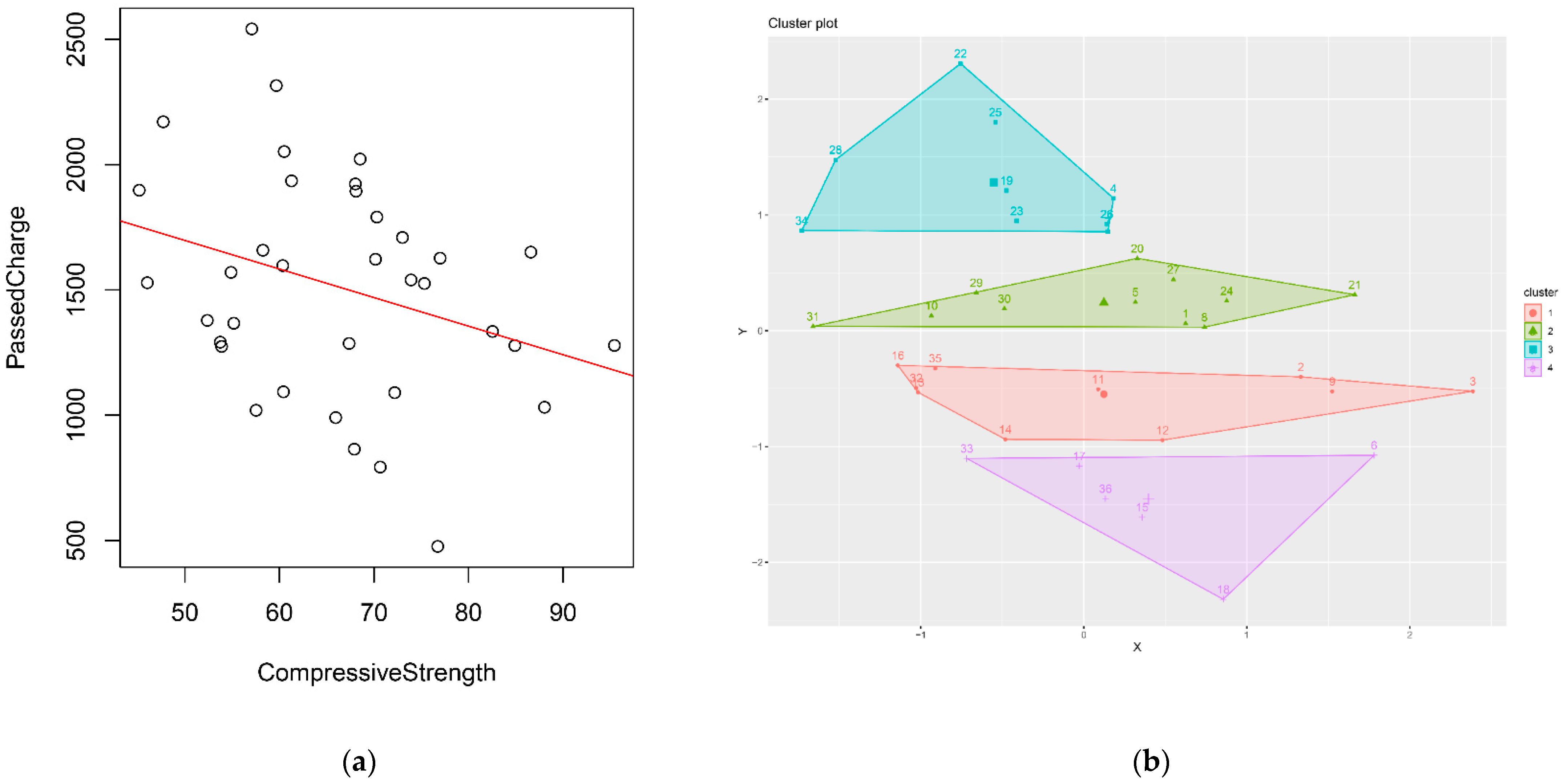
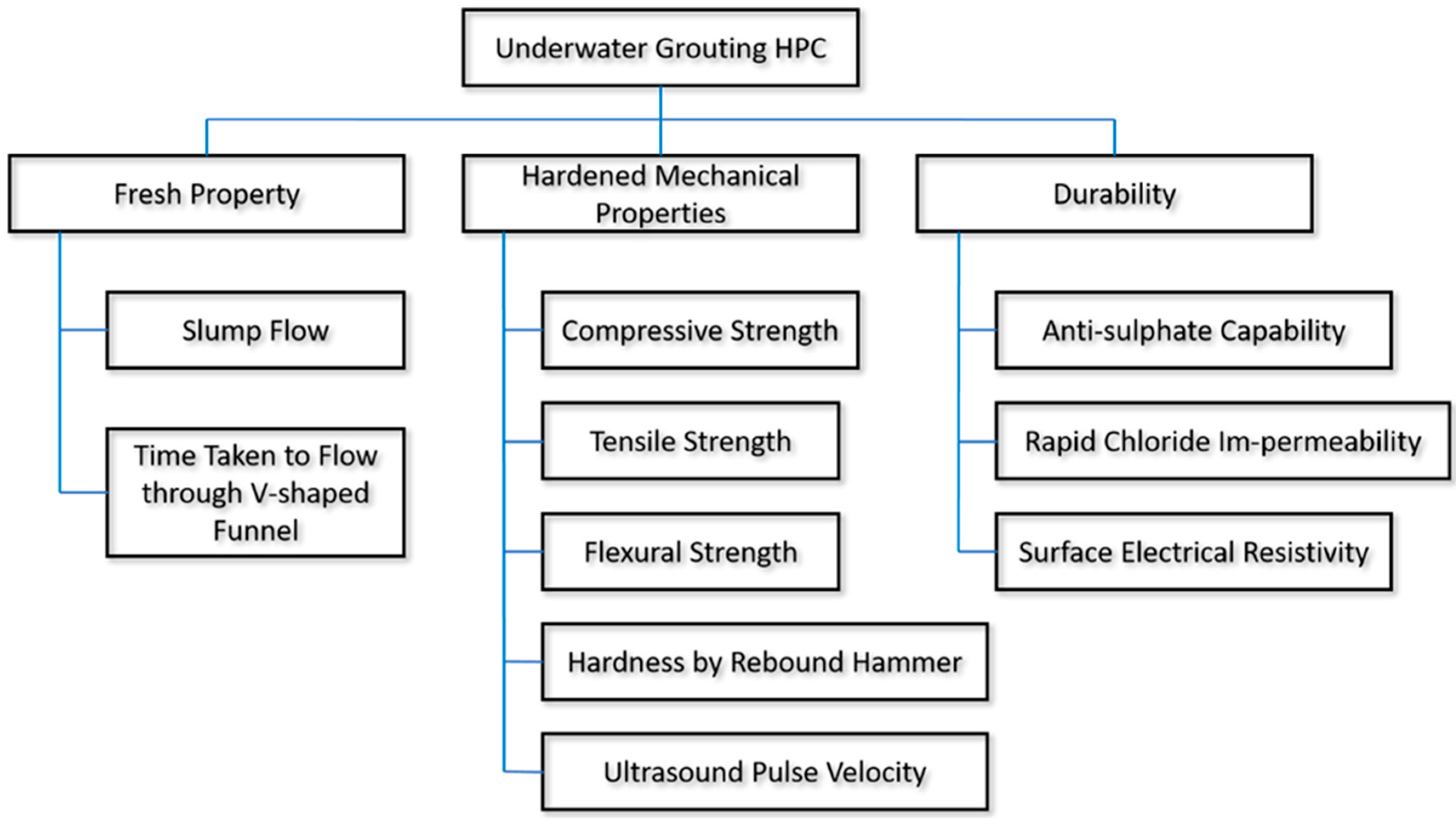
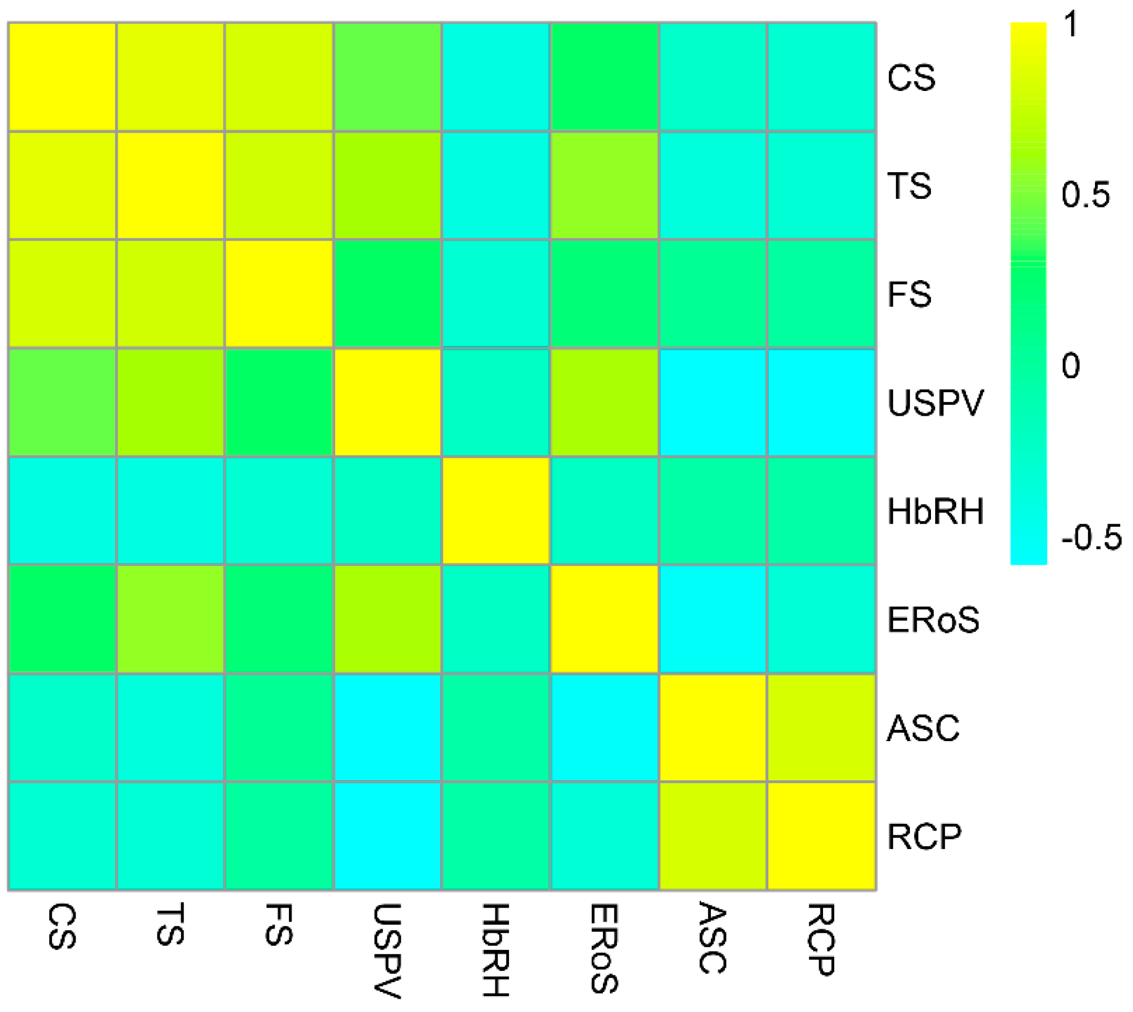
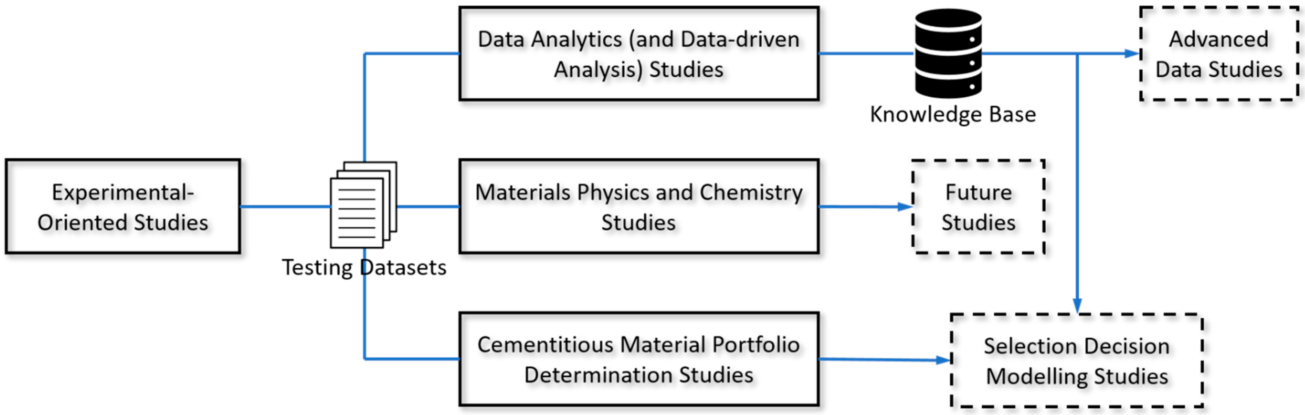
(a)
Parameter of HPC Sample		CS of Sample at Days (MPa)					TS of Sample at Days (MPa)
W/B Ratio	% of FA and SF	1	7	28	56	91	1	7	28	56	91
0.28	FA 0% SF 0%	42	65.3	73.92	82.54	95.43	7.32	12.74	16.15	17.24	22.05
	FA 0% SF 10%	31.7	56.3	68.53	70.16	88.04	5.39	9.82	12.86	15.16	21.04
	FA 10% SF 0%	28.2	60	68.1	75.33	84.9	4.28	10.29	13.13	15.33	19.57
	FA 10% SF 10%	27.1	46.4	54.88	67.37	72.19	4.41	8.8	10.69	14.89	18.81
	FA 20% SF 0%	27.9	42.5	53.88	60.42	70.66	4.17	7.17	8.8	12.29	14.95
	FA 20% SF 10%	25.8	40.5	52.37	65.95	76.74	3.71	6.94	8.2	12.31	17.89
0.30	FA 0% SF 0%	35.7	50.6	60.5	70.3	86.59	5.12	10.31	14.17	16.2	20.46
	FA 0% SF 10%	23.9	48	57.07	61.28	77	4.88	8.75	11.7	15.16	20.01
	FA 10% SF 0%	17.7	49.2	59.67	68.03	73.01	3.08	9.5	12.14	15.27	18.83
	FA 10% SF 10%	16.1	38.7	47.71	58.25	60.35	3.31	7.21	8.77	14.87	18.24
	FA 20% SF 0%	17	35.6	46.02	53.74	57.53	2.53	6.29	7.81	12.99	15.41
	FA 20% SF 10%	14.6	34.5	45.17	55.17	67.92	2.23	5.9	7.22	13.61	17.75
(b)
Parameter of HPC Sample		FS of Sample at Days (MPa)					HbRH of Sample at Days (MPa)
W/B Ratio	% of FA and SF	1	7	28	56	91	1	7	28	56	91
0.28	FA 0% SF 0%	6.29	11.66	13.49	13.74	14.21	37.61	36.58	33.09	31.26	27.92
	FA 0% SF 10%	3.79	9.79	10.5	12.18	12.48	45.41	42.57	43.68	40.36	33.37
	FA 10% SF 0%	6.54	10.62	10.77	12.31	13.39	53.47	50.51	44.97	43.24	37.17
	FA 10% SF 10%	4.8	8.79	9.95	10.84	11.71	58.47	55.56	50.42	52.23	45.45
	FA 20% SF 0%	5.64	8.37	10.05	10.56	10.82	63.48	65.68	59.89	60.78	57.55
	FA 20% SF 10%	3	7.56	8.93	9.35	10.18	37.61	36.58	33.09	31.26	27.92
0.30	FA 0% SF 0%	6.15	10.61	12.41	12.81	13.39	29.78	29.01	25.95	19.5	23.94
	FA 0% SF 10%	3.38	8.82	10.02	11.83	12.41	44.37	38.81	40.92	36.83	30.73
	FA 10% SF 0%	6.24	9.77	10.19	11.99	13.26	52.45	49.86	44.24	43.01	34.15
	FA 10% SF 10%	4.45	8.52	9.4	10.46	10.95	58	54.49	48.24	48.84	41.53
	FA 20% SF 0%	5.34	7.7	9.37	10.18	10.63	63.35	67.26	58.07	59.07	54.52
	FA 20% SF 10%	2.89	7.47	8.33	9.16	10.01	29.78	29.01	25.95	19.5	23.94
(c)
Parameter of HPC Sample		USPV of Sample at Days (m/s)					Weight Loss at Days for ASC (%)
W/B Ratio	% of FA and SF	1	7	28	56	91	28			56	91
0.28	FA 0% SF 0%	4263.7	4794.7	4923.3	5278	5653	5.07			3.35	0.57
	FA 0% SF 10%	3620.3	4135.3	4415.7	4781	4981.3	4.92			3.08	0.51
	FA 10% SF 0%	3816	4336.3	4545.7	4739.3	4859.7	4.81			2.47	0.27
	FA 10% SF 10%	3300.7	4380.3	4685	4773	4908.7	2.23			1.32	0.21
	FA 20% SF 0%	3389.3	3930.3	4313.7	5454.3	5823	2.21			1.28	0.18
	FA 20% SF 10%	3648.7	4167.3	4634.7	4910.7	5748.3	1.25			0.79	0.05
0.30	FA 0% SF 0%	4104	4598	4698	5236	5877.7	6.18			4.18	2.4
	FA 0% SF 10%	3442	3949	4359	5078.3	5287	5.76			4.15	2.03
	FA 10% SF 0%	3777.3	4384	4578.3	4815.3	5386.7	5.21			3.22	1.04
	FA 10% SF 10%	3308.7	4407.3	4612.7	4819.7	5338	3.31			2.3	0.71
	FA 20% SF 0%	3128	3786.3	4231.3	5342.3	6048	3.81			1.87	0.61
	FA 20% SF 10%	3423.3	3905.3	4593.7	5111.3	5993	2.41			1.94	0.3
(d)
Parameter of HPC Sample		Charge Passed for RCP (Coulombs)					ERoS Tested at Days (kΩ-cm)
W/B Ratio	% of FA and SF	28	56		91		1	7	28	56	91
0.28	FA 0% SF 0%	1539.7	1334		1278.36		21.43	25	37.89	77.11	93.11
	FA 0% SF 10%	2022	1622.1		1031.66		15.96	24.22	40.22	78.78	93.33
	FA 10% SF 0%	1893.7	1525.6		1277.91		14.03	25.44	40.67	77.78	93.44
	FA 10% SF 10%	1569.9	1286.3		1090.04		15.27	26.33	43	74.67	97.45
	FA 20% SF 0%	1274.3	1093.2		793.1		16.48	20.44	42.33	82	96.78
	FA 20% SF 10%	1378.3	990.4		476.593		22.02	28.89	47.33	76.33	93.33
0.30	FA 0% SF 0%	2051.9	1790.5		1650.65		25.67	46.92	72.44	82.78	98.53
	FA 0% SF 10%	2541.3	1934.9		1626.58		12.63	44.67	74.55	83.67	94.45
	FA 10% SF 0%	2315.2	1922.7		1709.15		11.96	46.22	71	82	90.67
	FA 10% SF 10%	2170.6	1658.2		1596.96		10.1	47.11	79.89	85.45	97.67
	FA 20% SF 0%	1528.6	1291.3		1019.57		16.6	41	77.22	79.22	98.78
	FA 20% SF 10%	1897.7	1366.8		864.455		27.76	58.72	81.45	94.89	98.33

Table 2. Correlation coefficients between each pair of variables (no transform).

	CS	TS	FS	USPV	HbRH	ERoS	ASC	RCP
CS	1	0.875333	0.824243	0.43716	−0.39808	0.29562	−0.2662	−0.31178
TS	0.875333	1	0.784765	0.622967	−0.40234	0.562644	−0.37139	−0.32165
FS	0.824243	0.784765	1	0.310713	−0.30525	0.205377	0.036492	−0.00205
USPV	0.43716	0.622967	0.310713	1	−0.23428	0.645174	−0.56893	−0.58283
HbRH	−0.39808	−0.40234	−0.30525	−0.23428	1	−0.23448	−0.04958	−0.05542
ERoS	0.29562	0.562644	0.205377	0.645174	−0.23448	1	−0.54312	−0.33091
ASC	−0.2662	−0.37139	0.036492	−0.56893	−0.04958	−0.54312	1	0.817532
RCP	−0.31178	−0.32165	−0.00205	−0.58283	−0.05542	−0.33091	0.817532	1

Table 3. Correlation coefficients between each pair of variables, with different RHS variable transforms: (a)

X^{'} = X^{2}

; (b)

X^{'} = X^{3}

; (c)

X^{'} = e^{X}

; (d)

X^{'} = 2^{X}

; (e)

X^{'} = \sqrt{X}

; (f)

X^{'} = \sqrt[3]{X}

; (g)

X^{'} = \log (X)

; (h)

X^{'} = \lg (X)

; (h) RHS Var. Transform:

X^{'} = \lg (X)

.

Table 3. Correlation coefficients between each pair of variables, with different RHS variable transforms: (a)

X^{'} = X^{2}

; (b)

X^{'} = X^{3}

; (c)

X^{'} = e^{X}

; (d)

X^{'} = 2^{X}

; (e)

X^{'} = \sqrt{X}

; (f)

X^{'} = \sqrt[3]{X}

; (g)

X^{'} = \log (X)

; (h)

X^{'} = \lg (X)

; (h) RHS Var. Transform:

X^{'} = \lg (X)

.

(a)	CS	TS	FS	USPV	HbRH	ERoS	ASC	RCP
CS	---	0.858867	0.816058	0.427017	−0.40513	0.30664	−0.27887	−0.30783
TS	0.880561	---	0.776248	0.605032	−0.42425	0.573121	−0.40888	−0.32631
FS	0.824674	0.77404	---	0.308186	−0.33502	0.203073	0.032173	−0.00081
USPV	0.423489	0.606038	0.292183	---	−0.22041	0.638643	−0.56441	−0.5831
HbRH	−0.42554	−0.42297	−0.33213	−0.18482	---	−0.20776	−0.07007	−0.10351
ERoS	0.331792	0.607924	0.221374	0.691903	−0.24499	---	−0.58517	−0.3763
ASC	−0.19251	−0.27938	0.063966	−0.502	−0.09105	−0.48745	---	0.748105
RCP	−0.31659	−0.32915	−0.05971	−0.55487	−0.05955	−0.29833	0.817113	---
(b)	CS	TS	FS	USPV	HbRH	ERoS	ASC	RCP
CS	---	0.835226	0.79966	0.414718	−0.40593	0.313178	−0.28814	−0.30018
TS	0.871874	---	0.754935	0.575965	−0.43141	0.566401	−0.43047	−0.32086
FS	0.822683	0.761367	---	0.30597	−0.36006	0.199425	0.027196	−0.00102
USPV	0.409015	0.588051	0.273135	---	−0.2067	0.630624	−0.55874	−0.5819
HbRH	−0.43656	−0.43129	−0.34513	−0.13617	---	−0.1822	−0.09105	−0.15006
ERoS	0.358293	0.639143	0.229501	0.725676	−0.25038	---	−0.61744	−0.41401
ASC	−0.15917	−0.22425	0.069324	−0.44791	−0.11265	−0.43577	---	0.686281
RCP	−0.31363	−0.32865	−0.106	−0.52188	−0.04927	−0.26239	0.790176	---
(c)	CS	TS	FS	USPV	HbRH	ERoS	ASC	RCP
CS	---	0.321631	0.336406	0.219982	−0.17004	0.133833	−0.17608	−0.08968
TS	0.592665	---	0.459743	0.280597	−0.25998	0.254154	−0.2681	−0.1505
FS	0.737376	0.6098	---	0.304023	−0.40063	0.144114	−0.04536	−0.04884
USPV	0.358691	0.526558	0.211007	---	−0.16596	0.597529	−0.53474	−0.56972
HbRH	−0.1884	−0.23478	−0.14302	0.057846	---	−0.09112	−0.11434	−0.20829
ERoS	0.084827	0.292588	0.036046	0.62018	−0.03992	---	−0.31469	−0.26921
ASC	−0.14749	−0.17135	0.0691	−0.3713	−0.14213	−0.32648	---	0.589916
RCP	−0.31593	−0.33037	−0.08779	−0.53969	−0.04701	−0.27681	0.800249	---
(d)	CS	TS	FS	USPV	HbRH	ERoS	ASC	RCP
CS	---	0.323844	0.337948	0.220534	−0.17107	0.135049	−0.17721	−0.09065
TS	0.6749	---	0.52721	0.330775	−0.3096	0.331323	−0.3241	−0.18401
FS	0.778735	0.667112	---	0.304588	−0.41544	0.163534	−0.01711	−0.0279
USPV	0.384434	0.557977	0.24204	---	−0.1861	0.615276	−0.54784	−0.57721
HbRH	−0.23342	−0.27959	−0.17728	0.037031	---	−0.11131	−0.11806	−0.23117
ERoS	0.10796	0.333232	0.039413	0.64	−0.04944	---	−0.36326	−0.30311
ASC	−0.1655	−0.21562	0.066715	−0.4307	−0.12331	−0.40243	---	0.665464
RCP	−0.31737	−0.33044	−0.06312	−0.55599	−0.05269	−0.29562	0.813711	---
(e)	CS	TS	FS	USPV	HbRH	ERoS	ASC	RCP
CS	---	0.880394	0.824872	0.441192	−0.392094	0.288458	−0.258755	−0.312252
TS	0.865763	---	0.782128	0.625573	−0.384953	0.549375	−0.346861	−0.314787
FS	0.822981	0.789199	---	0.312032	−0.288658	0.205933	0.038388	−0.003242
USPV	0.443633	0.630941	0.319695	---	−0.241226	0.647813	−0.570721	−0.582105
HbRH	−0.377150	−0.386542	−0.286130	−0.256779	---	−0.246965	−0.040729	−0.032930
ERoS	0.274790	0.535778	0.194523	0.618160	−0.227516	---	−0.520020	−0.306866
ASC	−0.317586	−0.422217	0.014438	−0.593223	−0.015192	−0.559757	---	0.840345
RCP	−0.305280	−0.313657	0.029273	−0.590432	−0.044729	−0.342215	0.801181	---
(f)	CS	TS	FS	USPV	HbRH	ERoS	ASC	RCP
CS	---	0.881580	0.824551	0.442364	−0.389739	0.285838	−0.256134	−0.312183
TS	0.861465	---	0.780105	0.625348	−0.378213	0.543715	−0.337961	−0.311825
FS	0.822392	0.790519	---	0.312473	−0.282887	0.206023	0.038979	−0.003723
USPV	0.445731	0.633517	0.322639	---	−0.243537	0.648594	−0.571243	−0.581773
HbRH	−0.369097	−0.380444	−0.278953	−0.263651	---	−0.250834	−0.038112	−0.025904
ERoS	0.267583	0.526391	0.190537	0.608824	−0.224994	---	−0.512241	−0.298850
ASC	−0.333218	−0.434350	0.008473	−0.595380	−0.001036	−0.558613	---	0.841635
RCP	−0.302340	−0.310183	0.039716	−0.591281	−0.039640	−0.344671	0.792474	---
(g)	CS	TS	FS	USPV	HbRH	ERoS	ASC	RCP
CS	---	0.883184	0.823110	0.444438	−0.384503	0.280268	−0.250707	−0.311714
TS	0.851240	---	0.774336	0.623212	−0.363411	0.530608	−0.319290	−0.304959
FS	0.820950	0.792906	---	0.313347	−0.271000	0.206050	0.040100	−0.004813
USPV	0.449834	0.638541	0.328445	---	−0.248149	0.650004	−0.572171	−0.580974
HbRH	−0.351451	−0.367043	−0.263505	−0.276192	---	−0.257982	−0.033478	−0.012764
ERoS	0.252926	0.507179	0.182086	0.589881	−0.219712	---	−0.496794	−0.283008
ASC	−0.352850	−0.440057	0.004440	−0.582619	0.031369	−0.536518	---	0.825594
RCP	−0.295152	−0.301861	0.060098	−0.589648	−0.027139	−0.347025	0.769558	---
(h)	CS	TS	FS	USPV	HbRH	ERoS	ASC	RCP
CS	---	0.883184	0.823110	0.444438	−0.384503	0.280268	−0.250707	−0.311714
TS	0.851240	---	0.774336	0.623212	−0.363411	0.530608	−0.319290	−0.304959
FS	0.820950	0.792906	---	0.313347	−0.271000	0.206050	0.040100	−0.004813
USPV	0.449834	0.638541	0.328445	---	−0.248149	0.650004	−0.572171	−0.580974
HbRH	−0.351451	−0.367043	−0.263505	−0.276192	---	−0.257982	−0.033478	−0.012764
ERoS	0.252926	0.507179	0.182086	0.589881	−0.219712	---	−0.496794	−0.283008
ASC	−0.352850	−0.440057	0.004440	−0.582619	0.031369	−0.536518	---	0.825594
RCP	−0.295152	−0.301861	0.060098	−0.589648	−0.027139	−0.347025	0.769558	---

Table 4. The Cos-Sim indices between each pair of variables (no transformation).

	CS	TS	FS	USPV	HbRH	ERoS	ASC	RCP
CS	1	0.991704	0.994792	0.986874	0.923028	0.970084	0.766091	0.929148
TS	0.991704	1	0.985801	0.978604	0.899398	0.974761	0.726442	0.906988
FS	0.994792	0.985801	1	0.990266	0.938099	0.971088	0.802627	0.951239
USPV	0.986874	0.978604	0.990266	1	0.947857	0.983320	0.771200	0.940099
HbRH	0.923028	0.899398	0.938099	0.947857	1	0.918275	0.765450	0.916059
ERoS	0.970084	0.974761	0.971088	0.983320	0.918275	1	0.712888	0.913845
ASC	0.766091	0.726442	0.802627	0.771200	0.765450	0.712888	1	0.909864
RCP	0.929148	0.906988	0.951239	0.940099	0.916059	0.913845	0.909864	1

Table 5. Results from estimating and developing the models (some initial entries).

M#	Y	X	P-Co-Co	$α^{*}$	$β^{*}$	$p (α^{*})$	$p (β^{*})$	p(M)	$R^{2}$	${(R^{2})}^{*}$
1	TS	CS	0.875333	−3.667713	0.278209	0.0466	0.0000	0.0000	0.766208	0.759331
2	TS	CS	0.858867	5.766322	0.001985	0.0000	0.0000	0.0000	0.737652	0.729936
3	TS	CS	0.835226	8.989167	0.000018	0.0000	0.0000	0.0000	0.697602	0.688708
4	TS	CS	0.321631	14.568831	0.000000	0.0000	0.0558	0.0558	0.103447	0.077077
5	TS	CS	0.323844	14.565644	0.000000	0.0000	0.0540	0.0540	0.104875	0.078548
6	TS	CS	0.880394	−22.324474	4.575331	0.0000	0.0000	0.0000	0.775094	0.768479
7	TS	CS	0.881580	−40.931240	13.814583	0.0000	0.0000	0.0000	0.777183	0.770630
8	TS	CS	0.883184	−62.850941	42.785409	0.0000	0.0000	0.0000	0.780015	0.773545
9	TS	CS	0.883184	−62.850941	12.879692	0.0000	0.0000	0.0000	0.780015	0.773545
10	FS	CS	0.824243	4.243931	0.104528	0.0000	0.0000	0.0000	0.679376	0.669946
11	FS	CS	0.816058	7.757808	0.000752	0.0000	0.0000	0.0000	0.665950	0.656125
12	FS	CS	0.799660	8.962874	0.000007	0.0000	0.0000	0.0000	0.639457	0.628852
13	FS	CS	0.336406	11.087036	0.000000	0.0000	0.0448	0.0448	0.113169	0.087086
14	FS	CS	0.337948	11.085907	0.000000	0.0000	0.0438	0.0438	0.114209	0.088156
15	FS	CS	0.824872	−2.696166	1.710449	0.1088	0.0000	0.0000	0.680414	0.671015
16	FS	CS	0.824551	−9.616035	5.155510	0.0004	0.0000	0.0000	0.679884	0.670469
17	FS	CS	0.823110	−17.693156	15.910370	0.0000	0.0000	0.0000	0.677510	0.668025
18	FS	CS	0.823110	−17.693156	4.789498	0.0000	0.0000	0.0000	0.677510	0.668025
19	USPV	CS	0.437160	3.857498	0.017583	0.0000	0.0077	0.0077	0.191108	0.167318
20	USPV	CS	0.427017	4.456269	0.000125	0.0000	0.0094	0.0094	0.182344	0.158295
21	USPV	CS	0.414718	4.659517	0.000001	0.0000	0.0119	0.0119	0.171991	0.147638
22	USPV	CS	0.219982	5.005173	0.000000	0.0000	0.1973	0.1973	0.048392	0.020403
23	USPV	CS	0.220534	5.004976	0.000000	0.0000	0.1962	0.1962	0.048635	0.020654
24	USPV	CS	0.441192	2.670380	0.290147	0.0027	0.0071	0.0071	0.194651	0.170964
25	USPV	CS	0.442364	1.485802	0.877204	0.2362	0.0069	0.0069	0.195686	0.172030
26	USPV	CS	0.444438	0.079830	2.724581	0.9630	0.0066	0.0066	0.197525	0.173923
27	USPV	CS	0.444438	0.079830	0.820181	0.9630	0.0066	0.0066	0.197525	0.173923
28	HBRH	CS	−0.398077	65.693972	−0.390663	0.0000	0.0162	0.0162	0.158465	0.133714
29	HBRH	CS	−0.405125	52.917551	−0.002891	0.0000	0.0142	0.0142	0.164126	0.139542
30	HBRH	CS	−0.405925	48.479311	−0.000027	0.0000	0.0140	0.0140	0.164775	0.140210
31	HBRH	CS	−0.170036	40.133608	0.000000	0.0000	0.3215	0.3215	0.028912	0.000351
32	HBRH	CS	−0.171068	40.138531	0.000000	0.0000	0.3185	0.3185	0.029264	0.000713
33	HBRH	CS	−0.392094	90.813888	−6.291765	0.0001	0.0180	0.0180	0.153738	0.128848
34	HBRH	CS	−0.389739	115.838473	−18.857628	0.0007	0.0188	0.0188	0.151897	0.126953
35	HBRH	CS	−0.384503	144.146418	−57.514972	0.0020	0.0206	0.0206	0.147843	0.122779
36	HBRH	CS	−0.384503	144.146418	−17.313732	0.0020	0.0206	0.0206	0.147843	0.122779
┇	┇	┇	┇	┇	┇	┇	┇	┇	┇	┇

Table 6. SLR models’ p values for each pair of variables, by different RHS variable transform methods: (a)

X^{'} = X^{2}

; (b)

X^{'} = X^{3}

; (c)

X^{'} = e^{X}

; (d)

X^{'} = 2^{X}

; (e)

X^{'} = \sqrt{X}

; (f)

X^{'} = \sqrt[3]{X}

; (g)

X^{'} = \log (X)

; (h)

X^{'} = \lg (X)

.

Table 6. SLR models’ p values for each pair of variables, by different RHS variable transform methods: (a)

X^{'} = X^{2}

; (b)

X^{'} = X^{3}

; (c)

X^{'} = e^{X}

; (d)

X^{'} = 2^{X}

; (e)

X^{'} = \sqrt{X}

; (f)

X^{'} = \sqrt[3]{X}

; (g)

X^{'} = \log (X)

; (h)

X^{'} = \lg (X)

.

(a)	CS	TS	FS	USPV	HbRH	ERoS	ASC	RCP
CS	0.000000	0.000000	0.000000	0.009394	0.014243	0.068910	0.099559	0.067789
TS	0.000000	0.000000	0.000000	0.000093	0.009916	0.000259	0.013286	0.052104
FS	0.000000	0.000000	0.000000	0.067451	0.045792	0.234888	0.852231	0.996245
USPV	0.010063	0.000090	0.083775	0.000000	0.196446	0.000028	0.000336	0.000190
HbRH	0.009670	0.010165	0.047811	0.280548	0.000000	0.224030	0.684669	0.548015
ERoS	0.048053	0.000084	0.194446	0.000003	0.149833	0.000000	0.000178	0.023698
ASC	0.260660	0.098907	0.710912	0.001811	0.597407	0.002567	0.000000	0.000000
RCP	0.059945	0.049972	0.729410	0.000445	0.730079	0.077182	0.000000	0.000000
(b)	CS	TS	FS	USPV	HbRH	ERoS	ASC	RCP
CS	0.000000	0.000000	0.000000	0.011907	0.014034	0.062907	0.088345	0.075272
TS	0.000000	0.000000	0.000000	0.000237	0.008612	0.000317	0.008775	0.056392
FS	0.000000	0.000000	0.000000	0.069549	0.031002	0.243582	0.874895	0.995302
USPV	0.013253	0.000162	0.107008	0.000000	0.226450	0.000037	0.000397	0.000197
HbRH	0.007769	0.008633	0.039253	0.428430	0.000000	0.287537	0.597416	0.382366
ERoS	0.031897	0.000027	0.178153	0.000001	0.140798	0.000000	0.000060	0.012067
ASC	0.353814	0.188561	0.687871	0.006154	0.513013	0.007894	0.000000	0.000004
RCP	0.062508	0.050343	0.538354	0.001097	0.775369	0.122102	0.000000	0.000000
(c)	CS	TS	FS	USPV	HbRH	ERoS	ASC	RCP
CS	0.000000	0.055766	0.044846	0.197340	0.321462	0.436468	0.304312	0.602958
TS	0.000140	0.000000	0.004788	0.097387	0.125694	0.134707	0.113898	0.380960
FS	0.000000	0.000079	0.000000	0.071435	0.015465	0.401719	0.792810	0.777263
USPV	0.031694	0.000970	0.216709	0.000000	0.333375	0.000119	0.000780	0.000287
HbRH	0.271163	0.168105	0.405339	0.737545	0.000000	0.597118	0.506679	0.222821
ERoS	0.622799	0.083328	0.834675	0.000055	0.817184	0.000000	0.061580	0.112349
ASC	0.390676	0.317673	0.688828	0.025775	0.408285	0.051972	0.000000	0.000153
RCP	0.060509	0.049079	0.610654	0.000681	0.785420	0.102184	0.000000	0.000000
(d)	CS	TS	FS	USPV	HbRH	ERoS	ASC	RCP
CS	0.000000	0.054008	0.043813	0.196189	0.318493	0.432274	0.301173	0.599052
TS	0.000006	0.000000	0.000954	0.048784	0.066138	0.048389	0.053810	0.282676
FS	0.000000	0.000009	0.000000	0.070884	0.011745	0.340585	0.921102	0.871662
USPV	0.020615	0.000406	0.154958	0.000000	0.277152	0.000065	0.000543	0.000228
HbRH	0.170646	0.098650	0.300968	0.830220	0.000000	0.518074	0.492845	0.174923
ERoS	0.530833	0.047033	0.819475	0.000026	0.774611	0.000000	0.029431	0.072328
ASC	0.334737	0.206599	0.699058	0.008735	0.473680	0.014964	0.000000	0.000009
RCP	0.059279	0.049027	0.714567	0.000430	0.760238	0.080032	0.000000	0.000000
(e)	CS	TS	FS	USPV	HbRH	ERoS	ASC	RCP
CS	0.000000	0.000000	0.000000	0.007071	0.018024	0.087981	0.127552	0.063732
TS	0.000000	0.000000	0.000000	0.000045	0.020430	0.000520	0.038214	0.061495
FS	0.000000	0.000000	0.000000	0.063928	0.087751	0.228218	0.824097	0.985030
USPV	0.006726	0.000037	0.057342	0.000000	0.156394	0.000019	0.000278	0.000196
HbRH	0.023359	0.019873	0.090691	0.130591	0.000000	0.146475	0.813553	0.848792
ERoS	0.104815	0.000758	0.255601	0.000059	0.182040	0.000000	0.001151	0.068695
ASC	0.059099	0.010315	0.933397	0.000137	0.929925	0.000386	0.000000	0.000000
RCP	0.070213	0.062484	0.865421	0.000150	0.795613	0.041055	0.000000	0.000000
(f)	CS	TS	FS	USPV	HbRH	ERoS	ASC	RCP
CS	0.000000	0.000000	0.000000	0.006903	0.018790	0.091034	0.131594	0.063793
TS	0.000000	0.000000	0.000000	0.000045	0.022941	0.000610	0.043804	0.064114
FS	0.000000	0.000000	0.000000	0.063534	0.094571	0.228012	0.821431	0.982807
USPV	0.006440	0.000034	0.054960	0.000000	0.152343	0.000019	0.000274	0.000198
HbRH	0.026739	0.022083	0.099447	0.120253	0.000000	0.140053	0.825341	0.880793
ERoS	0.114620	0.000975	0.265660	0.000081	0.187065	0.000000	0.001404	0.076639
ASC	0.047043	0.008122	0.960882	0.000128	0.995214	0.000399	0.000000	0.000000
RCP	0.073097	0.065603	0.818108	0.000146	0.818453	0.039532	0.000000	0.000000
(g)	CS	TS	FS	USPV	HbRH	ERoS	ASC	RCP
CS	0.000000	0.000000	0.000000	0.006615	0.020590	0.097797	0.140259	0.064214
TS	0.000000	0.000000	0.000000	0.000049	0.029361	0.000871	0.057676	0.070523
FS	0.000000	0.000000	0.000000	0.062757	0.109889	0.227950	0.816382	0.977773
USPV	0.005912	0.000028	0.050493	0.000000	0.144487	0.000018	0.000266	0.000203
HbRH	0.035566	0.027663	0.120466	0.102983	0.000000	0.128735	0.846305	0.941104
ERoS	0.136667	0.001594	0.287837	0.000153	0.197902	0.000000	0.002056	0.094423
ASC	0.034789	0.007237	0.979497	0.000193	0.855884	0.000743	0.000000	0.000000
RCP	0.080536	0.073575	0.727705	0.000154	0.875153	0.038117	0.000000	0.000000
(h)	CS	TS	FS	USPV	HbRH	ERoS	ASC	RCP
CS	0.000000	0.000000	0.000000	0.006615	0.020590	0.097797	0.140259	0.064214
TS	0.000000	0.000000	0.000000	0.000049	0.029361	0.000871	0.057676	0.070523
FS	0.000000	0.000000	0.000000	0.062757	0.109889	0.227950	0.816382	0.977773
USPV	0.005912	0.000028	0.050493	0.000000	0.144487	0.000018	0.000266	0.000203
HbRH	0.035566	0.027663	0.120466	0.102983	0.000000	0.128735	0.846305	0.941104
ERoS	0.136667	0.001594	0.287837	0.000153	0.197902	0.000000	0.002056	0.094423
ASC	0.034789	0.007237	0.979497	0.000193	0.855884	0.000743	0.000000	0.000000
RCP	0.080536	0.073575	0.727705	0.000154	0.875153	0.038117	0.000000	0.000000

Table 7. SLR models’ R² values for each pair of variables, by different RHS variable transform methods: (a)

X^{'} = X^{2}

; (b)

X^{'} = X^{3}

; (c)

X^{'} = e^{X}

; (d)

X^{'} = 2^{X}

; (e)

X^{'} = \sqrt{X}

; (f)

X^{'} = \sqrt[3]{X}

; (g)

X^{'} = \log (X)

; (h)

X^{'} = \lg (X)

.

Table 7. SLR models’ R² values for each pair of variables, by different RHS variable transform methods: (a)

X^{'} = X^{2}

; (b)

X^{'} = X^{3}

; (c)

X^{'} = e^{X}

; (d)

X^{'} = 2^{X}

; (e)

X^{'} = \sqrt{X}

; (f)

X^{'} = \sqrt[3]{X}

; (g)

X^{'} = \log (X)

; (h)

X^{'} = \lg (X)

.

(a)	CS	TS	FS	USPV	HbRH	ERoS	ASC	RCP
CS	---	0.737652	0.665950	0.182344	0.164126	0.094028	0.077766	0.094757
TS	0.775388	---	0.602560	0.366064	0.179988	0.328468	0.167184	0.106476
FS	0.680087	0.599138	---	0.094979	0.112237	0.041239	0.001035	0.000001
USPV	0.179343	0.367283	0.085371	---	0.048581	0.407865	0.318559	0.340004
HbRH	0.181081	0.178905	0.110312	0.034157	---	0.043164	0.004910	0.010714
ERoS	0.110086	0.369571	0.049006	0.478730	0.060021	---	0.342428	0.141604
ASC	0.037059	0.078054	0.004092	0.252008	0.008291	0.237607	---	0.559661
RCP	0.100227	0.108339	0.003565	0.307878	0.003547	0.088998	0.667674	---
(b)	CS	TS	FS	USPV	HbRH	ERoS	ASC	RCP
CS	---	0.697602	0.639457	0.171991	0.164775	0.098080	0.083026	0.090109
TS	0.760163	---	0.569927	0.331735	0.186118	0.320810	0.185304	0.102950
FS	0.676807	0.579680	---	0.093618	0.129642	0.039770	0.000740	0.000001
USPV	0.167293	0.345803	0.074603	---	0.042725	0.397687	0.312188	0.338609
HbRH	0.190586	0.186015	0.119115	0.018542	---	0.033196	0.008290	0.022518
ERoS	0.128374	0.408504	0.052671	0.526606	0.062689	---	0.381227	0.171407
ASC	0.025334	0.050289	0.004806	0.200628	0.012691	0.189895	---	0.470982
RCP	0.098363	0.108009	0.011236	0.272363	0.002428	0.068849	0.624378	---
(c)	CS	TS	FS	USPV	HbRH	ERoS	ASC	RCP
CS	---	0.103447	0.113169	0.048392	0.028912	0.017911	0.031003	0.008043
TS	0.351252	---	0.211364	0.078735	0.067590	0.064594	0.071876	0.022650
FS	0.543724	0.371856	---	0.09243	0.160501	0.020769	0.002057	0.002386
USPV	0.128659	0.277263	0.044524	---	0.027542	0.357041	0.285944	0.324581
HbRH	0.035494	0.055122	0.020455	0.003346	---	0.008304	0.013074	0.043385
ERoS	0.007196	0.085607	0.001299	0.384623	0.001594	---	0.099029	0.072474
ASC	0.021752	0.029362	0.004775	0.137867	0.020202	0.106588	---	0.348001
RCP	0.09981	0.109144	0.007707	0.291261	0.002210	0.076623	0.640398	---
(d)	CS	TS	FS	USPV	HbRH	ERoS	ASC	RCP
CS	---	0.104875	0.114209	0.048635	0.029264	0.018238	0.031402	0.008217
TS	0.455491	---	0.277951	0.109412	0.095853	0.109775	0.105039	0.033861
FS	0.606428	0.445038	---	0.092774	0.17259	0.026743	0.000293	0.000779
USPV	0.14779	0.311338	0.058583	---	0.034634	0.378565	0.300128	0.333176
HbRH	0.054487	0.078168	0.031428	0.001371	---	0.01239	0.013939	0.053442
ERoS	0.011655	0.111044	0.001553	0.409599	0.002444	---	0.131961	0.091879
ASC	0.02739	0.046491	0.004451	0.185503	0.015206	0.161951	---	0.442842
RCP	0.100725	0.109191	0.003984	0.309129	0.002776	0.087393	0.662126	---
(e)	CS	TS	FS	USPV	HbRH	ERoS	ASC	RCP
CS	---	0.775094	0.680414	0.194651	0.153738	0.083208	0.066954	0.097501
TS	0.749546	---	0.611724	0.391341	0.148188	0.301813	0.120312	0.099091
FS	0.677298	0.622835	---	0.097364	0.083323	0.042409	0.001474	1.05 × 10⁻⁵
USPV	0.19681	0.398086	0.102205	---	0.05819	0.419662	0.325723	0.338846
HbRH	0.142242	0.149415	0.08187	0.065935	---	0.060992	0.001659	0.001084
ERoS	0.075509	0.287058	0.037839	0.382121	0.051764	---	0.270421	0.094167
ASC	0.100861	0.178268	0.000208	0.351914	0.000231	0.313327	---	0.70618
RCP	0.093196	0.09838	0.000857	0.34861	0.002001	0.117111	0.64189	---
(f)	CS	TS	FS	USPV	HbRH	ERoS	ASC	RCP
CS	---	0.777183	0.679884	0.195686	0.151897	0.081703	0.065604	0.097458
TS	0.742121	---	0.608564	0.39106	0.143045	0.295626	0.114218	0.097235
FS	0.676328	0.624921	---	0.097639	0.080025	0.042445	0.001519	1.39 × 10⁻⁵
USPV	0.198676	0.401344	0.104096	---	0.05931	0.420674	0.326318	0.33846
HbRH	0.136233	0.144737	0.077815	0.069512	---	0.062918	0.001453	0.000671
ERoS	0.071601	0.277087	0.036304	0.370667	0.050622	---	0.262391	0.089311
ASC	0.111034	0.18866	7.18 × 10⁻⁵	0.354477	1.07 × 10⁻⁶	0.312048	---	0.70835
RCP	0.091409	0.096214	0.001577	0.349613	0.001571	0.118798	0.628015	---
(g)	CS	TS	FS	USPV	HbRH	ERoS	ASC	RCP
CS	---	0.780015	0.67751	0.197525	0.147843	0.07855	0.062854	0.097166
TS	0.724609	---	0.599596	0.388393	0.132067	0.281544	0.101946	0.093
FS	0.673959	0.6287	---	0.098187	0.073441	0.042456	0.001608	2.32 × 10⁻⁵
USPV	0.20235	0.407734	0.107876	---	0.061578	0.422505	0.327379	0.337531
HbRH	0.123518	0.13472	0.069435	0.076282	---	0.066555	0.001121	0.000163
ERoS	0.063972	0.25723	0.033155	0.347959	0.048274	---	0.246804	0.080094
ASC	0.124503	0.19365	1.97 × 10⁻⁵	0.339445	0.000984	0.287851	---	0.681605
RCP	0.087115	0.09112	0.003612	0.347684	0.000737	0.120426	0.592219	---
(h)	CS	TS	FS	USPV	HbRH	ERoS	ASC	RCP
CS	---	0.780015	0.67751	0.197525	0.147843	0.07855	0.062854	0.097166
TS	0.724609	---	0.599596	0.388393	0.132067	0.281544	0.101946	0.093
FS	0.673959	0.6287	---	0.098187	0.073441	0.042456	0.001608	2.32 × 10⁻⁵
USPV	0.20235	0.407734	0.107876	---	0.061578	0.422505	0.327379	0.337531
HbRH	0.123518	0.13472	0.069435	0.076282	---	0.066555	0.001121	0.000163
ERoS	0.063972	0.25723	0.033155	0.347959	0.048274	---	0.246804	0.080094
ASC	0.124503	0.19365	1.97 × 10⁻⁵	0.339445	0.000984	0.287851	---	0.681605
RCP	0.087115	0.09112	0.003612	0.347684	0.000737	0.120426	0.592219	---

Table 8. Simplified and visualised information for Table 2.

	CS	TS	FS	USPV	HbRH	ERoS	ASC	RCP
CS	—	0.875333	0.824243	0.43716	−0.39808
TS	0.875333	—	0.784765	0.622967	−0.40234
FS	0.824243	0.784765	—	0.310713	−0.30525
USPV	0.43716	0.622967	0.310713	—	−0.23428
HbRH	−0.39808	−0.40234	−0.30525	−0.23428	—
ERoS						—	−0.54312	−0.33091
ASC						−0.54312	—	0.817532
RCP						−0.33091	0.817532	—

Publisher’s Note: MDPI stays neutral with regard to jurisdictional claims in published maps and institutional affiliations.

© 2022 by the authors. Licensee MDPI, Basel, Switzerland. This article is an open access article distributed under the terms and conditions of the Creative Commons Attribution (CC BY) license (https://creativecommons.org/licenses/by/4.0/).

Share and Cite

MDPI and ACS Style

Zhuang, Z.-Y.; Kuo, W.-T. Unravelling the Relations between and Predictive Powers of Different Testing Variables in High Performance Concrete Experiments: The Data-Driven Analytical Methods. Buildings 2022, 12, 1545. https://doi.org/10.3390/buildings12101545

AMA Style

Zhuang Z-Y, Kuo W-T. Unravelling the Relations between and Predictive Powers of Different Testing Variables in High Performance Concrete Experiments: The Data-Driven Analytical Methods. Buildings. 2022; 12(10):1545. https://doi.org/10.3390/buildings12101545

Chicago/Turabian Style

Zhuang, Zheng-Yun, and Wen-Ten Kuo. 2022. "Unravelling the Relations between and Predictive Powers of Different Testing Variables in High Performance Concrete Experiments: The Data-Driven Analytical Methods" Buildings 12, no. 10: 1545. https://doi.org/10.3390/buildings12101545

Note that from the first issue of 2016, this journal uses article numbers instead of page numbers. See further details here.

Article Menu

Unravelling the Relations between and Predictive Powers of Different Testing Variables in High Performance Concrete Experiments: The Data-Driven Analytical Methods

Abstract

1. Introduction

2. Literature Review and Methods

2.1. Background of the Problem

2.1.1. Renewable Energy (RE) Planning and Wind Farm Construction

2.1.2. The Special Weather/Sea Conditions in Taiwan and the Effects for Wind Turbines

2.2. About the Parameters

2.2.1. Compressive Strength (CS)

2.2.2. Tensile Strength (TS)

2.2.3. Flexural Strength (FS)

2.2.4. Hardness (by Rebound Hammer) (HbRH)

2.2.5. Ultrasound Pulse Velocity (USPV)

2.2.6. Anti-Sulphate Capability (ASC)

2.2.7. Rapid Chloride (Im-)Permeability (RCP)

2.2.8. Electrical Resistivity on Surface (ERoS)

2.3. The Methods: A Brief Review

2.3.1. Correlation Analysis

2.3.2. Cosine Similarity Analysis

2.3.3. Simple Linear Regression

2.3.4. Data Variable Transforms

2.3.5. Indicators Used to Justify the SLR Modelling Results

3. Results

3.1. Original Datasets

3.2. Correlation Analysis

3.3. Cosine Similarity Analysis

3.4. Regression Analysis

3.5. Additional Information

4. Insights and Discussions

4.1. For Method Applications

4.1.1. Insights for Data Pre-Processing Results

4.1.2. Insights for Correlation Analysis Results

4.1.3. Insights from the Results of the Cosine-Similarity Analysis

4.1.4. Insights from the Established SLR Models

The Established ‘Knowledge Base’ Is Novel and Benefits Future HPC Sample Testing

A Method Is Provided to Explore the Insights into the Variables That Can Practically Be Used to Predict Another Variable and to Determine How Accurate the Prediction Will Be

Another Perspective to View the Model Information Is Offered to Differentiate and Recommend the Appropriate Transforms to Be Used for a Variable

4.1.5. Other Insights from the Research

4.2. Theory-Linking

5. Conclusions

Author Contributions

Funding

Data Availability Statement

Conflicts of Interest

Acronyms (Alphabetic Order)

Appendix A

Appendix B

Appendix C

References

Share and Cite

Article Metrics

Article Access Statistics

Further Information

Guidelines

MDPI Initiatives

Follow MDPI