1. Introduction
Almost all real fire experiments involve the temperature measurement with thermocouples. There are many of types of thermocouples which differ in the material used, the range of measured temperature and application. Regardless of these differences all thermocouples work due to the Seebeck effect. Thanks to the low costs and apparent simplicity of measurement it is possible to sample values of temperature in many locations within the examined volume. However, contrary to common belief the process of temperature measurement is complex and it may be that the recorded value differs significantly from the real hot gas temperature [
1]. This especially concerns unsteady cases and is mainly caused by the thermal inertia of the thermocouple bead under turbulent, fluctuating fire conditions [
2]. The thermocouple bead diameter is of great importance here [
3]. The commonly admitted analytical model of a thermocouple takes into account different heat transfer mechanisms [
4]. Although the governing phenomena had been already studied long ago [
5], the issue is still an object of intensive research. For instance, a comprehensive work was recently presented by Liu et al. [
6]. Hence, to explain some of the observed divergences between the measured and calculated temperatures [
7], the numerical investigation on the temperature measurement process is included in the presented work. The novel approach allows for the simultaneous modeling of thermocouples with different bead diameters as if they are located in every cell of the computational domain.
Sprinkler systems are an integral part of many fire safety strategies [
8,
9]. In order to work, sprinklers must activate early enough so that the size of the fire has not exceeded a certain design value. If the fire size is beyond this value by the time of activation, the water discharge from the activated sprinkler head will not be able to control the fire. Traditionally, adequate activation is achieved by following prescriptive guidance, e.g., the NFPA 13 standard [
10], where the type and sprinkler head distribution is indicated. The working principle of automatic sprinkler heads is quite simple: the nozzle is blocked by a removable link (e.g., a glass bulb filled with some liquid) that is heated by the hot gas flowing past, and eventually breaks.
Under certain circumstances (e.g., in the presence of automatically activated natural vents) a sprinkler system laid out according to standardized guidance might not provide optimal protection, and it could be beneficial to be able to assess the layout using numerical simulations of different fire scenarios. Węgrzyński et al. developed a methodology that allows for identifying the locations of sprinkler head placements based on 3D activation maps [
11]. Furthermore, since sprinklers are usually mounted just beneath a compartment ceiling, the temperature distribution in this region has a crucial significance for proper activation as well [
12].
While some of the earliest fire models were specifically developed for the estimation of heat detector activation time (sprinkler heads can be thought of as a type of heat detector), these models are experimental correlations with a limited range of applicability [
13].
The first attempt of predicting sprinkler activation times using a Computational Fluid Dynamics (CFD) fire model was made by Tuovinen [
14], who used the CFD code JASMINE and implemented the original
RTI model but neglected conductive losses to the sprinkler mounting. The latter factor has been included in Fire Dynamics Simulation (FDS) from the very beginning. Works on the validation of the sprinkler activation times were presented by McGrattan et al. [
15] and Olenick et al. [
16].
A more detailed model, accounting for smoke accumulation under the ceiling was used by Wade et al., who compared calculated activation times to the activation times measured at a specially designed full-scale experiment [
17,
18]. They found that their model over-predicted activation times by 21% on average, which can be attributed partially to the limited spatial resolution of the model.
Hopkin et al. [
19] conducted a comparative study to assess the capability of the FDS software to estimate sprinkler activation time, using the same experimental data obtained by Bittern [
18]. They considered different numerical settings (fire area, grid size, value of C-factor), and found that while sprinkler activation times are still generally over-predicted, the relative difference between experiments and simulations can be reduced to less than 10%. An interesting aspect of Hopkin’s study is that they report consistent over-prediction of the gas phase temperature at sprinkler locations when compared to experimental results.
For general purpose assessment of sprinkler activation with spatial resolution, it is convenient to use CFD models that are capable of reproducing the flow and temperature fields in fire scenarios to an acceptable level of accuracy. This is a challenging task, as fire simulations rely on a complex interaction of fluid dynamics and combustion processes and many decisions regarding the model set up need to be made.
In this study an alternative use of CFD models of thermocouple response and sprinklers activation is proposed. The introduced approach is implemented via a set of user defined functions (UDF) within ANSYS Fluent (v. 2019 R1). This allowed for the simultaneous modeling of many types of sprinkler heads and thermocouples of different diameters as if they are located in every cell of the computational domain in a single simulation run. The advantage is the ability for simultaneous examination of the whole volume, while previously this would have been performed with multiple point-measuring devices. This allows for multi-variant analyses of fire safety systems. This will make it easier to plan sprinkler placement for engineers designing sprinkler systems for a building. On the other hand, a thorough analysis of the operation of thermocouples will be important information for researchers designing and performing fire experiments. These benefits simply require smart extension of the commonly applied software. The integrated model was validated using the data provided by experiments conducted by Bittern and described in detail by Hopkin et al. [
18,
19]. The results were also compared to those obtained with FDS software (v. 6.7.6).
The rest of the paper is organized as follows. First the real fire experiments carried out by Bittern are described. Next, the foundations of numerical modeling of RTI approach and principles of modeling of the temperature measurement process are discussed. This is followed by the description of the entire numerical model with details specific to fire modeling. This concerns both Fluent and FDS models. The results section provides the direct outcomes of the work, and then a wider discussion is included. The conclusions section ends the work.
2. Materials and Methods
The outcomes of the presented work have been validated using data coming from a series of 22 experiments for the assessment of sprinkler activation times, which were conducted by Bittern in 2004 [
18].
2.1. Experimental Research on Sprinkler Activation
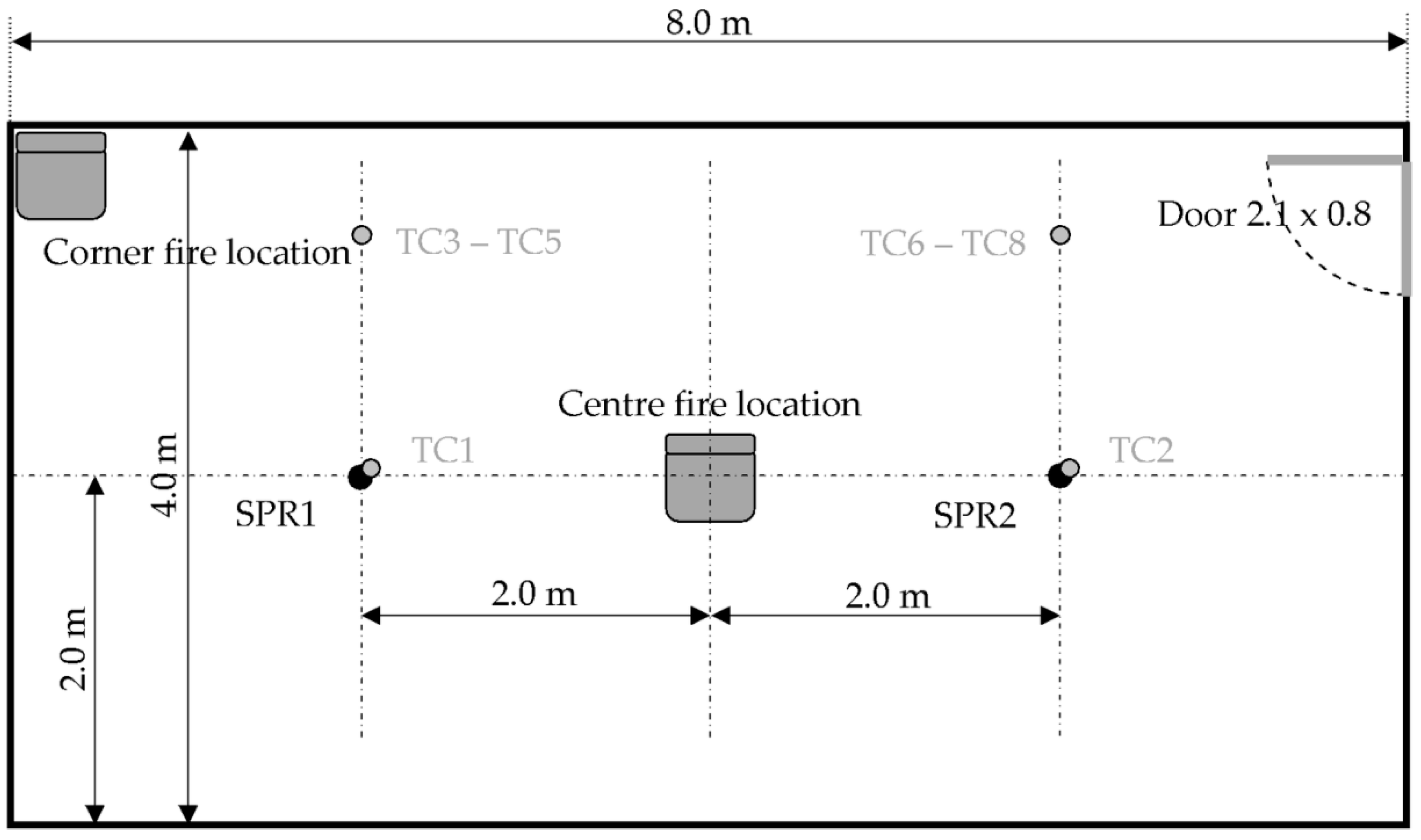
The tests were carried out in standardized gypsum wallboard compartment that was 4 m wide and 8 m long, with a height of 2.4 m. The A door 2.1 m high and 0.8 wide was placed on the short wall. The burning items were two polyurethane foam slabs (mimicking a chair) covered in fabrics, of 0.5 m × 0.4 m × 0.1 m in size. The back and bottom plates were made of solid plasterboard. The base of the seat was at a height of 0.65 m. The experimental layout is shown in
Figure 1. Two fire locations were tested: the first in the middle of the room, and the second in the corner opposite the doors (as indicated in
Figure 1). During the tests, two door positions were examined: shut and open. Two K thermocouple trees were placed along the longer wall neighboring the doors. The thermocouples were located at heights of 1.0 m, 2.1 m and 2.3 m above the floor. Additionally, two sprinkler heads and two thermocouples were mounted at the ceiling on the longer symmetry axis of the room, 2 m away from the walls (as indicated in
Figure 1).
Four types of sprinkler heads were used. They are shown in
Table 1. Two kinds of polyurethane foam, which differed in effective combustion heat (
EHC) were applied: F1 with
EHC = 21.0 MJ/kg and F2 with
EHC = 20.4 MJ/kg. Solid petroleum firelighters of size of 0.02 m × 0.02 m × 0.01 m were used to start the fire.
The burning chair was placed on a load cell with 5-gram increment. It allowed for precise mass loss monitoring, which in turn determined the current heat release rate (HRR).
Successive fire tests differed in details, like fire location, door open or shut, sprinkler type or polyurethane foam used. Configurations of all 22 fire tests are shown in
Table 2. The experiments (quite expectedly) demonstrated that sprinkler heads with the same activation temperature but different
RTI activated at different times (lower
RTI resulting in earlier detection), and that sprinklers with the same
RTI but different activation temperatures also activated at different times. They further showed that the distance of the fire to the sprinkler has an important influence on the activation time of the sprinkler head. The influence of opening the doors could not be conclusively determined. Test #11 failed due to record equipment malfunction and therefore was not taken into account in the following numerical simulations (it is marked by gray background in
Table 2 and then in Table 7).
2.2. Foundations of Numerical Modeling of Heat Sensors
Generally, two types of heat sensors were modeled in this work: automatic sprinklers and thermocouples. In both cases an unsteady process was considered—the inflowing gas with a time variant temperature heated the device head. The rate of head temperature change depends on many parameters, including head construction details. Therefore two well recognized analytical models were applied.
2.2.1. Sprinkler Bulb Model
The thermal properties of a sprinkler head are summarized in a single value called the response time index (
RTI) [
20]. Due to the relatively small dimensions of the link and its high conductivity, the Biot number (a ratio of the heat transfer resistances inside of a body and at the surface of a body) is much less than the unity (about 0.1 to 0.2), and lumped heating of the link by the hot combustion gases can be assumed [
21].
If heat losses to the sprinkler fitting are taken into consideration [
22], the following expression for the link temperature (
Te) emerges, in which the
RTI quantity (m
1/2s
1/2) describes generally a sprinkler sensitivity:
where
u is the velocity of the hot gases,
Tg is their temperature,
T0 is the temperature of the sprinkler fitting and
C is a constant ((m/s)
1/2) related to heat transfer properties of the sprinkler head [
23]. The first term corresponds to heat transfer between the sprinkler head and fluid, the second term corresponds to conduction by sprinkler mounting. Since sprinklers are expected to be activated in the early stage of a fire, when the inner structure of a room should remain unheated, commonly the initial temperature is adopted as
T0. The considered model was experimentally evaluated by Frank et al. [
24]. Similar but equivalent approaches were presented by other researchers [
25,
26]. As gas temperature and velocity in the case of fire are generally not constant, it is necessary to solve the equation numerically [
27,
28]. Although Equation (1) was derived semi-empirically in a static experiment it can be applied here only if the adopted time step is short enough. User defined memory (UDM) slots are used to store the three variables related to the problem: recent time step, previous bulb temperature, and activation indicator. This allows for calculation of the bulb temperature increment (
dTe) in consecutive time steps. Calculation stops for a given cell when the head reaches the activation temperature, and the activation indicator is then set. Using multiple triples of memory slots, many types of sprinklers can be assessed at the same simulation.
2.2.2. Thermocouple Model
The experiments referred to resulted also in data on temperature coming from measurements by thermocouples. As such, the real temperature recorded can be compared with the temperature calculated by ANSYS Fluent. However, one should be aware that the calculated fluid temperature cannot be directly considered here, because temperature measuring devices show their own temperature, and in a transient case such a system might not be in thermodynamic equilibrium. As a fire develops, the temperature increases in different ways for different locations of the analyzed space. A thermocouple is immersed in the fluid and the heat is transferred from fluid by conduction, convection and radiation. These processes do not complete immediately, so the thermocouple response is delayed in relation to the temperature of the surrounding fluid. It may even happen that due to the unstable nature of fire, the temperature of a thermocouple is temporarily higher than the fluid, so the heat transfer momentarily proceeds in the opposite direction. Thus, accurate temperature comparison is required to build a thermocouple model. This was done in two different modes:
analytical mode, in which a differential equation describing the thermocouple response was introduced, and
physical mode, in which a thermocouple was modeled just as a metal nugget.
For the analytical mode the following equation governing heat exchange between a thermocouple and its surroundings was used [
29]:
where:
Vtc and Atc—volume and surface area of the thermocouple (m3 and m2 respectively),
ρtc and ctc—density and specific heat (kg/m3 and J/kg∙K respectively),
Ttc and Tf—thermocouple and local fluid temperature (K),
I—incident radiative flux (to the thermocouple, W/m2),
εtc—thermocouple emissivity (0.85),
σB—the Stefan–Boltzmann constant (5.64 10−8 W/m2K4)
h—heat transfer coefficient (W/m2K).
The heat transfer coefficient
h was obtained from Nusselt number [
5]:
where:
For ball-shaped thermocouples
D is just its diameter, for cylindrical heads
D is the base diameter and the height. The quotient
Atc/
Vtc is equal to 6/
D in both cases. In the considered problem the Nusselt number is expressed as a combination of the Prandtl number and the Reynolds number, as follows (
µ is fluid dynamic viscosity, kg/m∙s):
The presented approach requires two additional memory slots (UDM) for each mesh cell (finite volume): the first one for the previous time step and the second for the previous thermocouple temperature. In this way the temperature, which would be measured by a thermocouple placed in a given cell, is calculated for the entire fluid volume.
The second mode of thermocouple modeling lacks this advantage, because it requires putting a model of a real thermocouple head in a given location. As a result, a metal nugget of the required shape and dimensions is modeled. This obviously entails the necessity of applying a dense enough mesh for these selected locations. Hence, this approach is not so comfortable as the previous one, but was used for comparison purposes.
2.3. CFD Modeling of the Experiments
The computational domain for the CFD simulations corresponded to the real room. The arrangement of all important elements was also reproduced. The burning chair was modeled as two fluid volumes, corresponding to the seat and backrest, respectively. The porosity was applied to both parts, which imitated the real polyurethane foam. The back and bottom plates were modeled as solid plasterboard.
Since Bittern reported that even for tests with a closed door the fire developed briskly and never reached the under-ventilated state, the fuel controlled fire model was assumed. Therefore a species transport model was adopted for fire modeling. The ‘source terms’ option was enabled for porous volumes of seat and backrest. This means that it was possible to establish bulk sources of some quantities with controlled generation rates. Sources of energy, water vapor, carbon dioxide and soot were set to relevant values, which resulted from the adopted combustion reaction. Since the soot yield was estimated as 22.7% [
19,
30], the following simplified reaction was considered (nitrogen transformations were completely neglected):
The mass balance of this reaction determined the produced amounts of carbon dioxide, water vapor and soot. Values are shown in
Table 3.
The fire curves (HRR vs. time) provided by Hopkin [
19] were sampled and stored in a text file as piecewise linear relations. A dedicated UDF was created, which at successive time steps read the sampled data and interpolated it. Then, according to known
EHC the fuel mass loss was determined (depending on the foam type) and in turn using the aforementioned mass balance the instantaneous masses of combustion products were calculated too. In such a way the volumes of the combustible parts of the chair emitted combustion products and energy to reliably simulate the real fire.
Since strong buoyancy forces were engaged in the examined phenomena the gravity was enabled and set to 9.81 m/s
2. The real experiment description provided the estimation of total leakage of the test compartment (independently on the door state open/shut). A circular vent of the ‘pressure outlet’ type boundary condition was introduced to mimic this. Its area was 0.053 m
2, which equaled the reported value. The door, when open, was also modeled as a ‘pressure outlet’ boundary condition. Due to enabled gravity the applied ambient pressure had to decrease with height (
z coordinate), hence an additional UDF was used to control the pressure profile at these boundary conditions (
g denotes gravitational acceleration):
Considering fire issues, one must take into account radiative energy transport. If it is assumed that at position
in the direction
the radiation of intensity
I (W/m
2) passes a layer of an absorbing, emitting, and scattering medium with a thickness of
ds, and the general equation describing the radiative transport can be expressed as follows [
31]:
The optical properties of the medium are described by a, σs, and n, which denote, respectively, the absorption coefficient (1/m), the scattering coefficient (1/m) and the refractive index. The phase function Φ describes the scattering process of radiation incoming at direction into direction (this function depends on the fluid nature and properties). The scattered radiation is integrated over the full solid angle Ω’.
As significant amounts of soot, carbon dioxide and water vapor were expected, the fluid had to be treated as optically dense. Therefore the discrete ordinate (DO) radiation model was applied. It solves the full radiative transport equation given above for each finite volume, hence it requires significant computational resources, but it is the most accurate [
31]. For the same reasons, the DO model is used in the well-recognized FDS package [
32]. Additionally, it is able to pass to a UDF the exact radiative flux through each cell, which is desirable for the thermocouple modeling. Since soot is the dominant source and sink of thermal radiation, and its properties are not particularly sensitive to wavelength, the radiation was regarded as grey.
All of the mentioned UDFs were called at every iteration, however this did not result in an observable increase of the computation time. The principal assumptions for numerical calculations and the choice of physical sub-models are summarized in
Table 4.
3. Results
Since the results may be affected by the structure of a numerical mesh and the adopted turbulence model, some preliminary calculations were done. This allowed not only for adjusting the numerical model, but first of all some general tips for compartment fires modeling were found.
3.1. Numerical Mesh and Study on Its Sensitivity
The modeled experiments were carried out for different assembly configurations, and thus, mainly due to different locations of the burning chair, two series of mesh analyses were done. Applied meshes were created following the guidelines presented by Węgrzyński et al. [
33]. Since the accuracy of the simulated flow within the ceiling boundary layer is crucial for the examined phenomena, the mesh in this region should consist of fine elements, which are able to capture gradients of flow variables. This was ensured by introducing a number of inflation layers along the ceiling–layers of thin cells, which thickness gradually increased with the distance from this no-slip wall.
Table 5 contains the data of the applied meshes. Unstructured meshes (containing only tetrahedrons) and structural meshes (containing mostly hexahedral cells) were examined as well.
The meshes used occasionally for simulating a physical head of a thermocouple consisted of slightly more elements due to the need to accurately capture the small size of these devices. The head region was meshed into a number of tiny cells and in its vicinity the cell size gradually increased until it fit the cells in the bulk. Thus, in this approach it was possible to model thermocouples just in a few locations determined in advance.
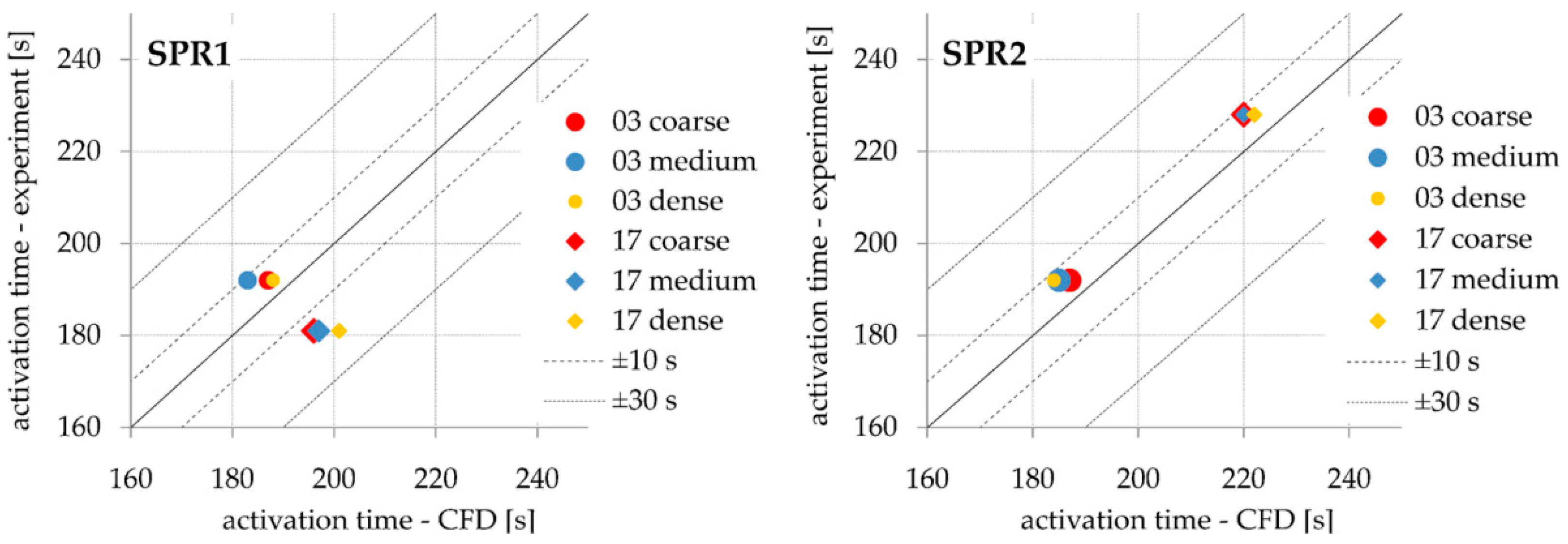
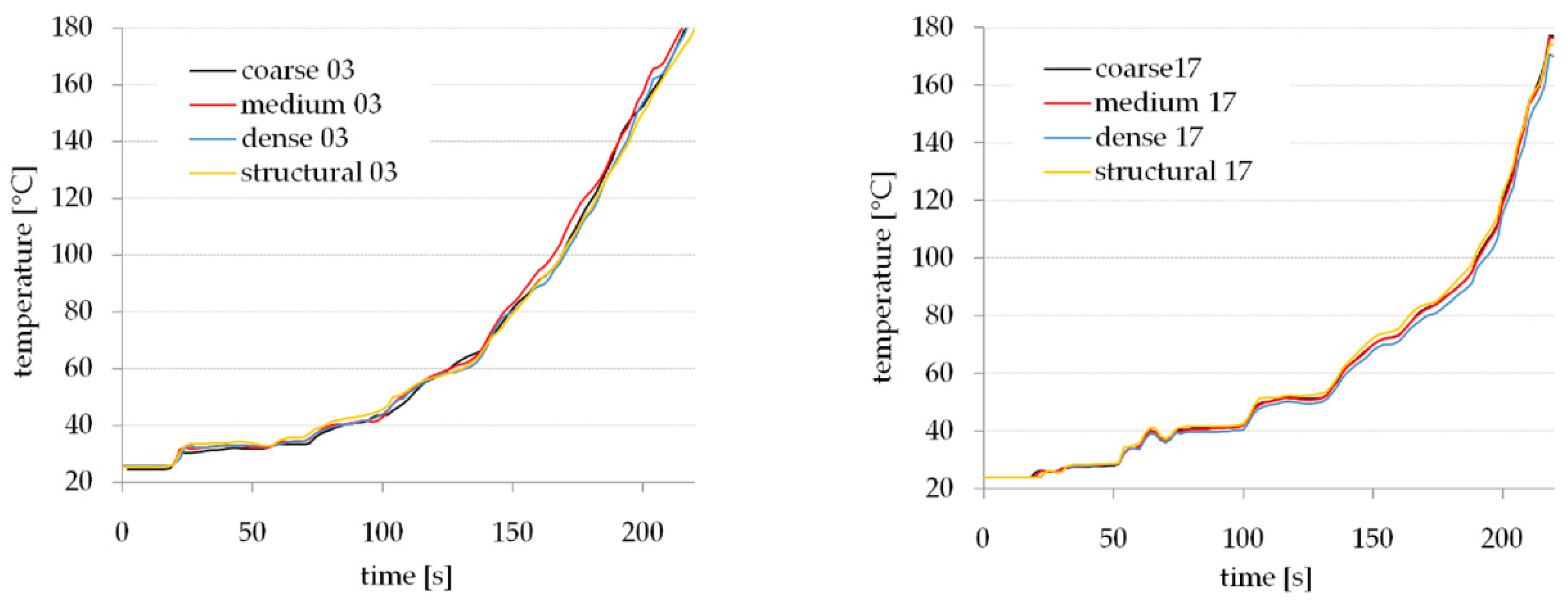
The data which were taken into account when considering the influence of the mesh structure were calculated sprinkler activation times and the time dependence of calculated temperature at the sprinklers locations. Given the large simulation output, only selected results are shown. These are the results for experiment #03 (fire in the middle of the room and door opened) and experiment #17 (fire in the left upper corner and door shut).
Figure 2 presents calculated sprinkler activation times compared to the measured times and
Figure 3 presents the time dependence of the calculated temperature.
As it can be seen, the mesh selection did not significantly impact the results. Both the calculated temperature and calculated sprinklers activation times seem to be independent of mesh density, and hence the numerical model can be regarded as robust.
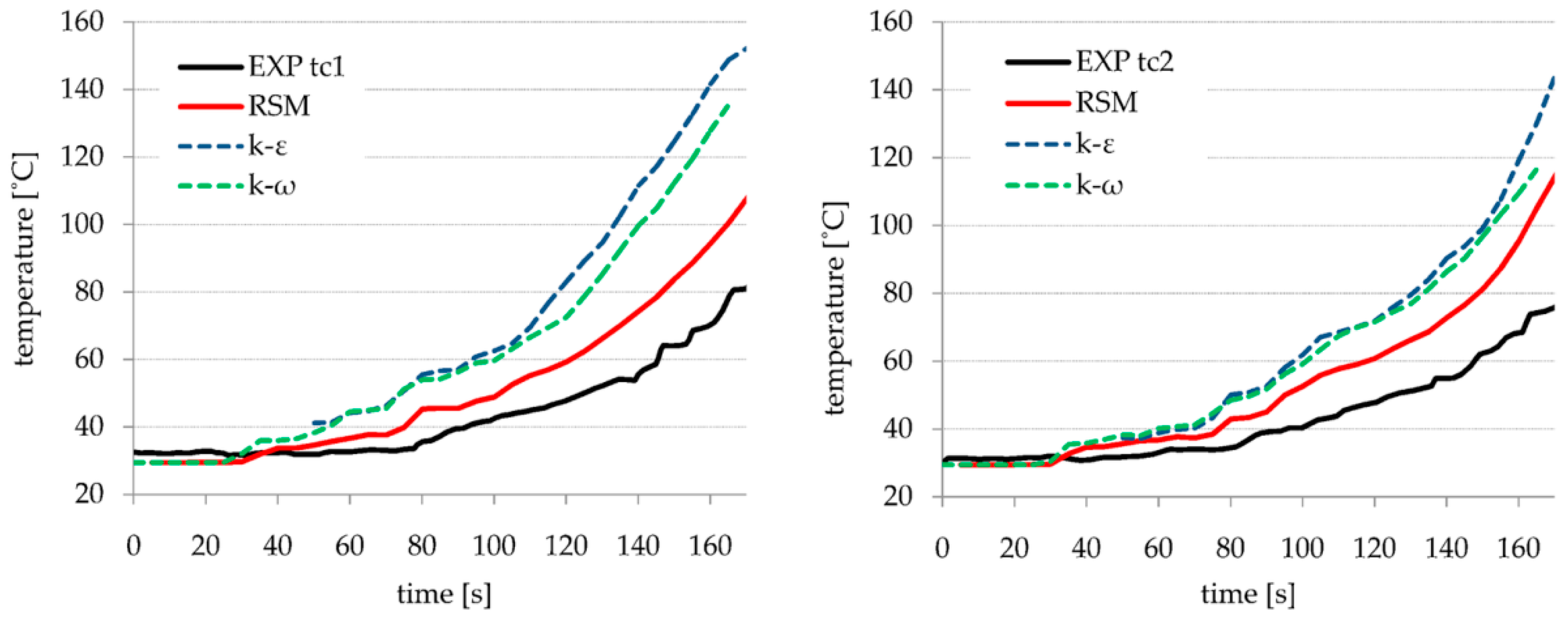
3.2. Turbulence Model Sensitivity Analysis
Some preliminary outcomes of the work suggested the need to examine the performance of different turbulence models. The problem arose when two well recognized (
k-
ω SST and
k-
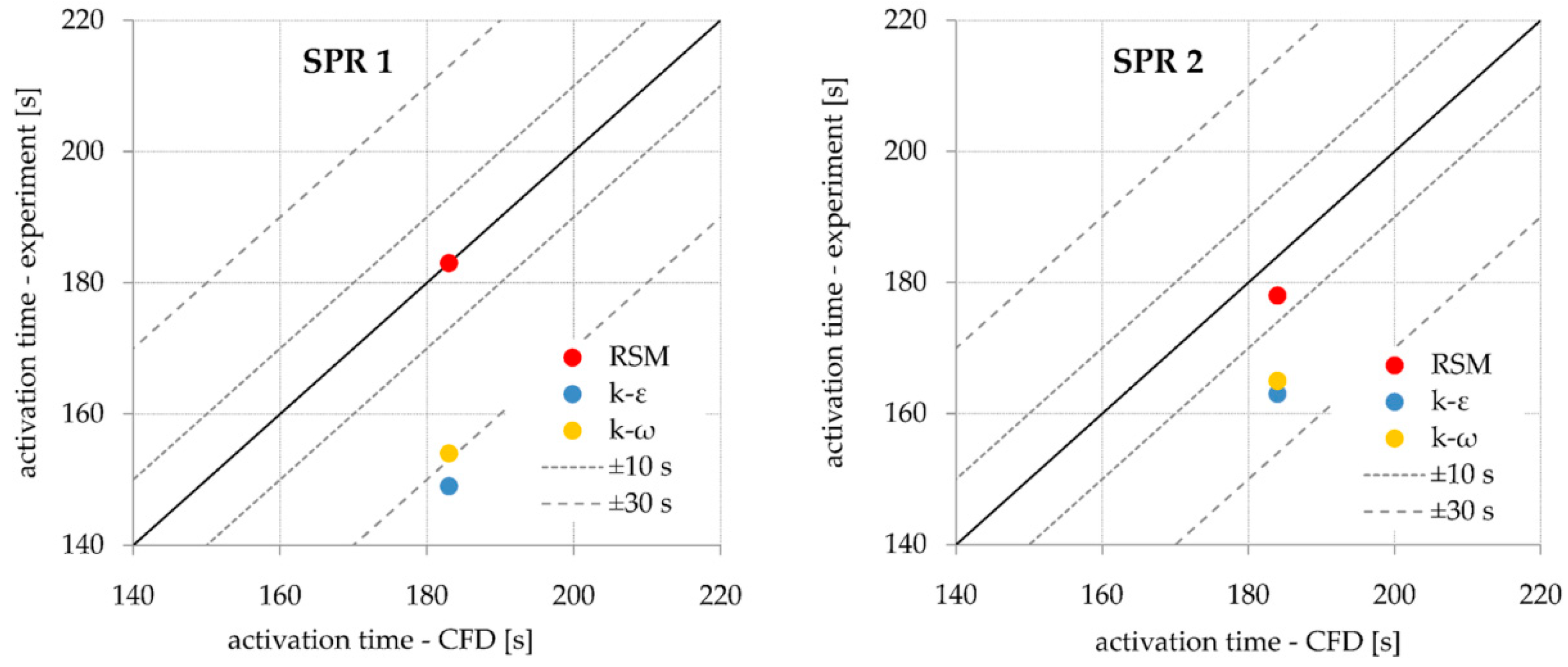
ε Realizable) turbulence models were routinely applied and then compared with the RSM (Reynold’s Stress Model) turbulence model. An example is shown in
Figure 4 as a juxtaposition of calculated and measured sprinkler activation times for Experiment #10. The same concerned the results of other experiments and furthermore, all calculated temperature distributions compared with the measured values.
Both
k-
ω and
k-
ε models predicted significantly shorter activation times for other experiments as well. This was due to the clearly overestimated temperature, as shown in
Figure 5. This observation may seem astonishing since both models are widely used in fire research analyses [
34].
Although, the temperature predicted by the RSM turbulence model seems also to be higher than experimentally measured, one must have in mind that the experimental curve represents the temperature measured by a thermocouple and the calculated values correspond to the gas temperature. This issue will be discussed later in detail.
The observed divergences could be explained by considering the mathematical foundations of the applied turbulence models. All models mentioned here belong to the RANS (Reynolds Averaged Navier–Stokes) family of turbulence models. The main assumption for these models is the so-called Reynolds approximation, which states that the instantaneous fluid velocity (
ui) is a sum of the average velocity (
) and fluctuating velocity (
) [
35]:
By definition, the time average of the fluctuating component equals zero:
Inserting this into the original equations governing the fluid flow leads to an alternative equations system in terms of the sought averaged velocities. A consequence of the averaging is the appearance of a new unknown quantity, called the Reynold’s tensor of viscous stresses (N/m
2). Being a symmetric tensor, it contains six variables:
In the RSM this equation system is directly solved, but six additional conservation equations for the tensor components are needed and an additional one is required for the turbulence kinetic energy (
k). This may result in high requirements in terms of computational resources. However, due to the high accuracy when modeling complex, anisotropic flows with violent changes of fluid velocity and bulk forces, it is a viable alternative [
35].
A further simplification, based on the Boussinesq’s hypothesis provides turbulence models, which are commonly recognized as science and industry standards. Here, the components of the tensor of viscous stresses are expressed by a single quantity, called turbulent viscosity [
36]. Worth noticing is the fact that the possible flow anisotropy is disregarded at the point. In the main, the turbulent energy transport is here regarded in a similar way as the molecular energy transport. Then, depending on some differences, two kinds of these models were developed:
k-ε, in which turbulent viscosity is determined by turbulence kinetic energy (
k) and dissipation rate of turbulence energy (
ε), and
k-ω, in which the turbulent viscosity is determined by the turbulence kinetic energy and turbulence frequency (
ω).
All of the above allowed for a deeper understanding of why k-ε and k-ω models failed in the considered case. When modeling a developing fire, one can observe the plume of hot gases which rise up until it reaches the ceiling due to buoyancy forces. When hitting the ceiling, the hot gases have to divert rapidly and start to spread along the ceiling. This description perfectly fits the circumstances for which the RSM model performance is better suited than other turbulence models.
3.3. Fire Dynamic Simulator Model
Since researchers and, above all, practitioners who deal with fire development and fire safety issues use the commonly well-recognized FDS package, models for all considered cases were also examined using this software. FDS uses the large eddy simulation (LES) turbulence model by default. This approach assumes a direct numerical solution of the Navier–Stokes equations for the largest vortices, and the smallest vortices, smaller than the size of a single computational cell, are analytically modeled [
37].
First, two mesh densities were checked to find the optimal mesh, and moreover a denser mesh was applied to the layer under the ceiling for better modeling the flows in this crucial region.
Table 6 presents the FDS meshes which were examined.
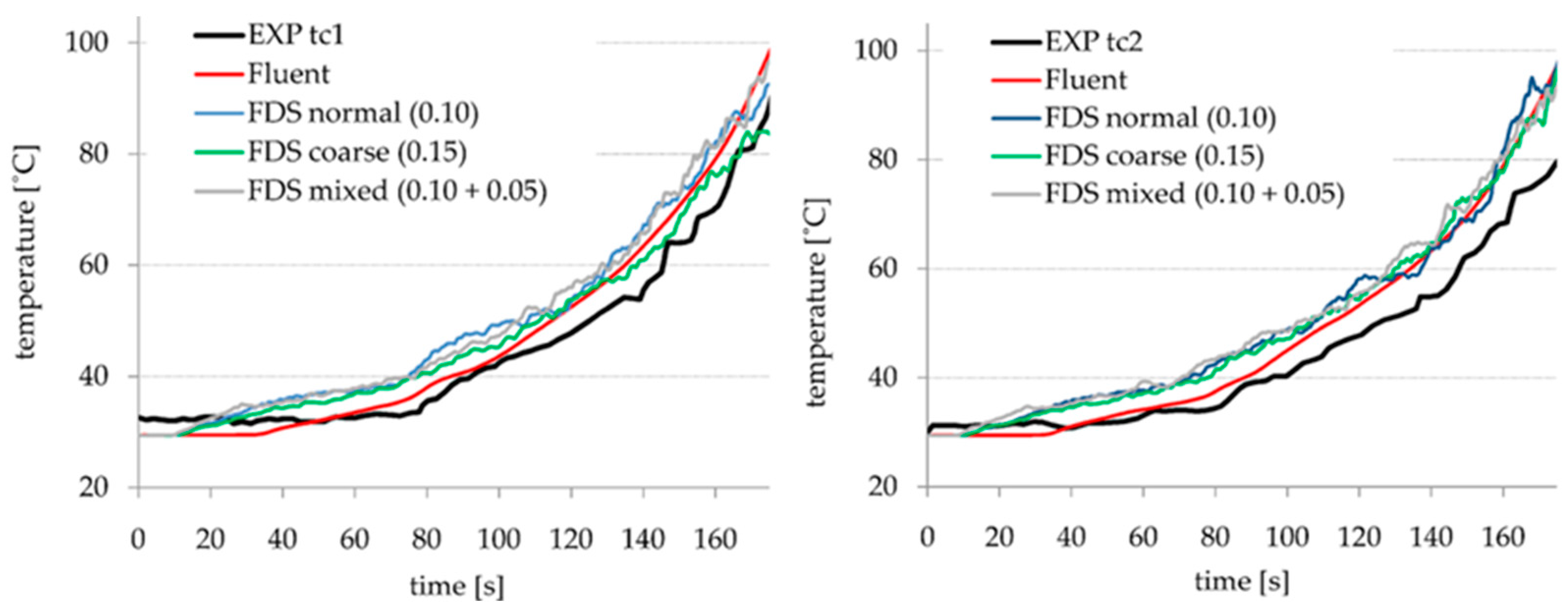
Figure 6 shows the outcomes of the FDS simulation for experiment #10: temperature recorded by thermocouples TC1 and TC2 compared with the experimental data and the Fluent results for thermocouple analytical model (which will be discussed later). As one can see, all presented data are consistent and they agree with the experimental results. The FDS model appeared to be mesh independent and, finally, the homogenous mesh of cell size of 0.1 m was applied for further simulations.
3.4. Results and Discussion
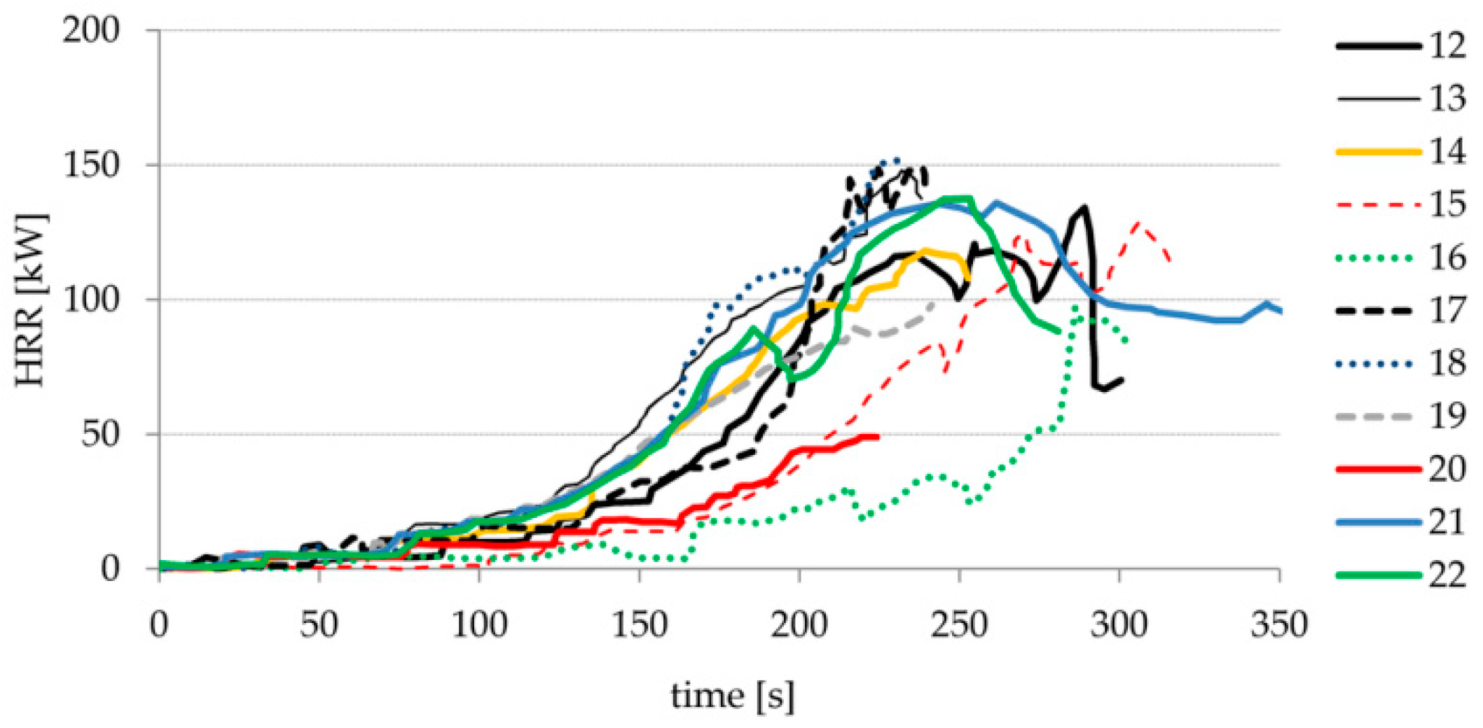
The approach described above was used for sprinkler and thermocouple modeling at the same time. The data were obtained for both devices, as if they had been placed in any cell of the computational domain. The numerical simulations were carried out for all cases reported by Bittern [
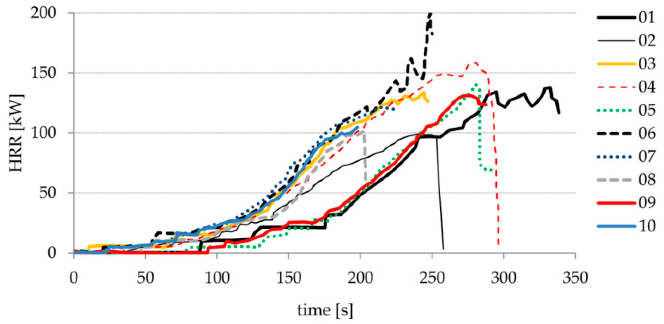
18] using Fluent with the RSM turbulence model and using FDS software too. This allowed for a satisfactory validation of adopted model assumptions. Whenever possible, all the results are presented, but some considerations have to be limited to a single case due to the large amount of data. Despite the controlled conditions of the experiments carried out, the unpredictable nature of fire results in significantly different curves of HRR. They are carefully reproduced in the CFD simulations presented here.
Figure 7 and
Figure 8 present the calculated HRR curves for both experiment groups (which differed in the
EHC of used polyurethane foam).
3.4.1. Results of Sprinklers Activation Modeling
In this section the results concerning sprinklers SPR1 and SPR2 are considered. The sprinkler parameters were adopted according to the data in
Table 1 and
Table 2. The sprinklers are assumed to be mounted 0.015 m below the ceiling. Since the value of the
C parameter may differ from the nominal value (0.4) by up to 10%, values of
C = 0.35 and
C = 0.45 were checked as well. It was possible, thanks to the ability of the proposed approach, to examine many sprinkler types at the same time. All results concerning sprinklers activation times for the nominal value of the
C parameter are presented in
Table 7. If a table entry is left blank, a sprinkler was not activated during an experiment or a simulation.
As can be easily seen, excluding a few exceptions, the calculated activation times are generally close to the measured ones. These exceptions with significantly greater errors were cases 16–22, for which the door was shut and the fire source was located in the corner. For Fluent and FDS simulations, as in the case of #16, both sprinklers were not activated at all, and the other activation times are a bit overestimated for the sprinkler SPR1. The Fluent results for the sprinkler SPR2 do not differ from the real ones (excluding case #21, for which the real activation time seems to be somehow outstanding). Although the FDS results are in general accordance with real data and with the Fluent results for the middle fire source location (cases 1–15), the predicted activation times for the corner fire source location are significantly overestimated, or even sprinklers were not activated at all. Some error indicators were calculated for the presented data: root mean squared error (
RMSE–Equation (11)), mean absolute error (
MAE–Equation (12)) and the mean absolute percentage error (
MAPE–Equation (13)). Quantity
nc denotes the number of considered cases in each dataset, terms
ta,CFD and
ta,real denote calculated and real activation times, respectively. If a real sprinkler was not activated (case #20, SPR2), the case is not taken into account. If a simulated sprinkler was not activated, the total simulation time (340 s) is inserted into these formulas. The synthetic overview of the results accuracy is presented in
Table 8.
The above error values confirm the conclusions from
Table 7: although for normally structured flows (middle fire location), both CFD packages perform with similar accuracy, for more complex flows (corner fire location), FDS performs significantly worse.
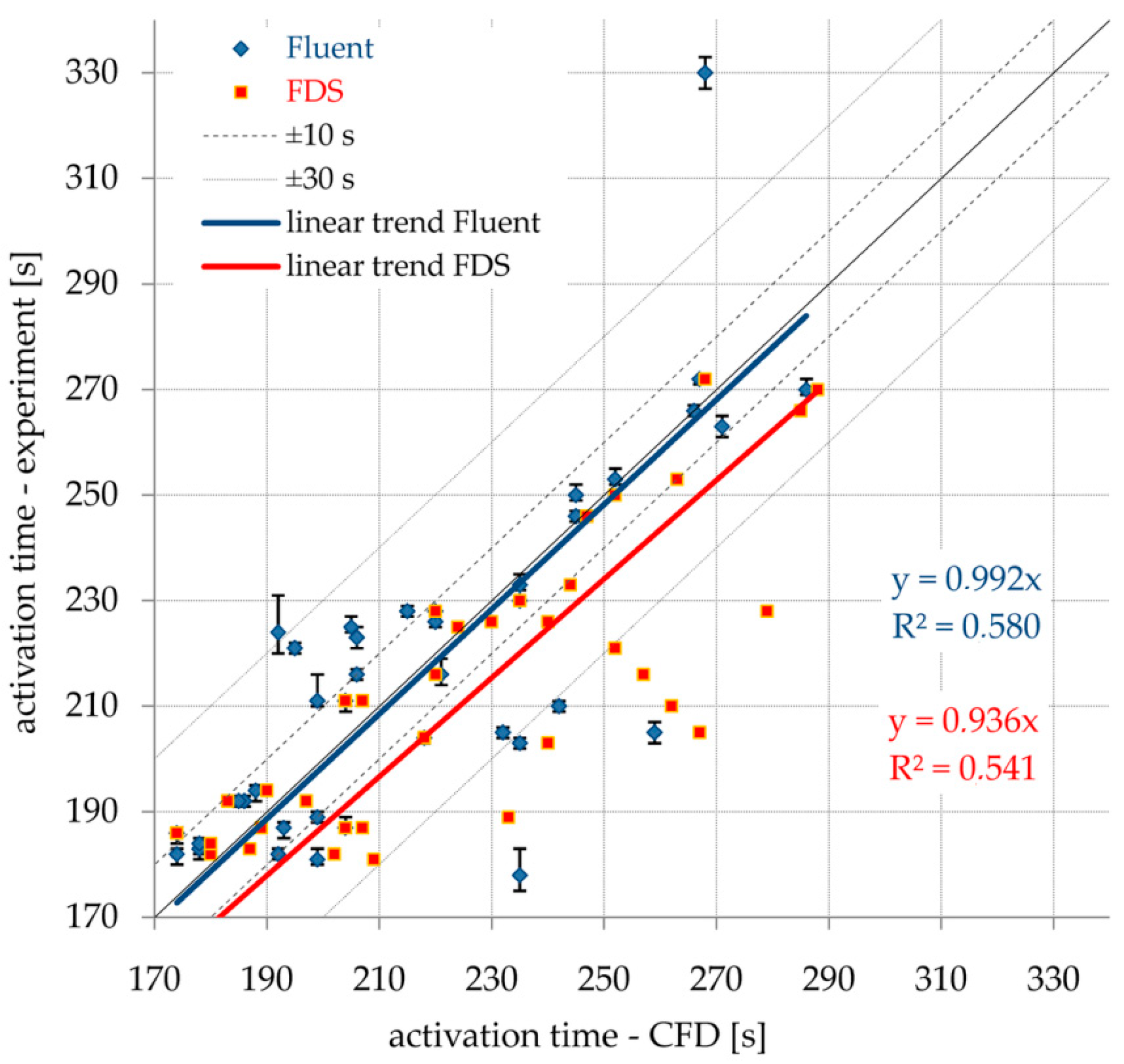
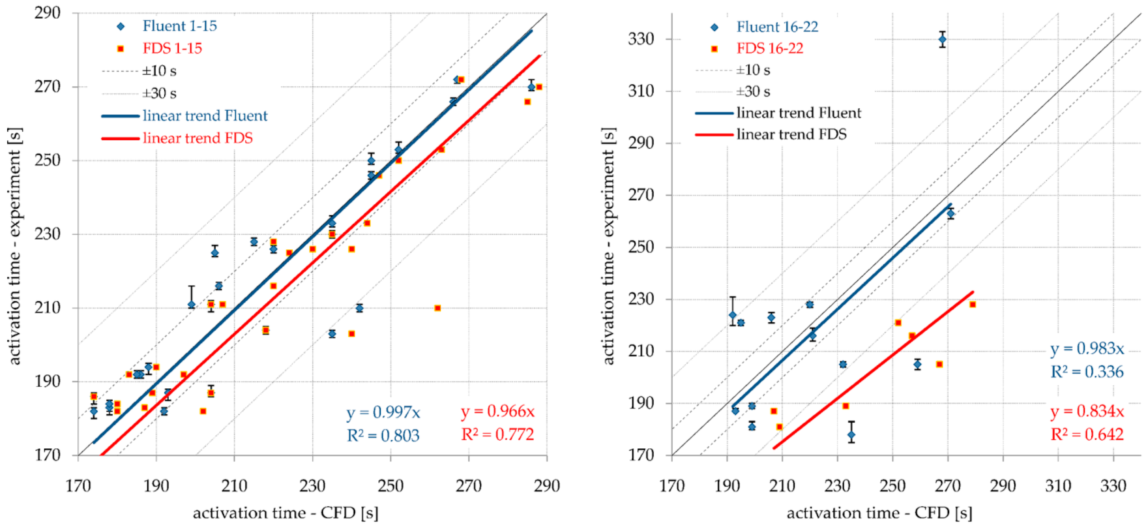
Figure 9 presents the results for sprinklers SPR1 and SPR2 together in a diagram form. Since the results for both fire locations differed they are presented separately in
Figure 10 again. Vertical error bars correspond to the range of activation times calculated using Fluent for
C1 values of 0.35 to 0.45. This was possible thanks to the ability of the presented approach to examine many sprinkler types at once.
Clear linear trends can be determined for both considered series. Almost all Fluent data-points fit the band ±10 s. The FDS data-points are also well bunched but their trend is a bit deviated towards longer times than the real ones. Just a few data-points fell outside of the band of ±30 s. The parameters of linear trends for both series also proves the overall modeling accuracy; data from Fluent gave the relation with determination coefficient R2 = 0.580. For FDS data, the relation and determination coefficient R2 = 0.541 were obtained. This validates the assumptions of both models, but indicates a significant spread of the calculated data as well.
The results for the middle fire location match the experimental data well. This is confirmed by the parameters of linear trends for both series: data from Fluent gave the relation , which is almost the perfect fit with the determination coefficient R2 = 0.803. For FDS data, the relation and determination coefficient R2 = 0.772 were obtained, which also testifies to the good quality of the numerical modeling.
The results for the corner fire location do not fit the experimental data so perfectly. However the Fluent data-points still keep the linear trend with the gradient very close to 1.0 (), but they are scattered to a significant degree—the determination coefficient value is quite low R2 = 0.336. The linear trend for FDS data-points is deviated significantly, as the relation is just . This series seems to be a bit better bunched (R2 = 0.642), but one should have in mind that there are just a few FDS data-points in this series. This is because, for this fire location, the sprinklers were often not activated at all in the FDS simulation, and this was especially the case for the sprinkler SPR2, which was further from the fire.
Although these discrepancies might result mainly from some numerical modeling deficiencies, they could be also caused by real sprinklers parameters scatter or from other factors, like air humidity [
38] (which were not taken into account). However, despite some isolated exceptions, the results can be regarded as reliable in general.
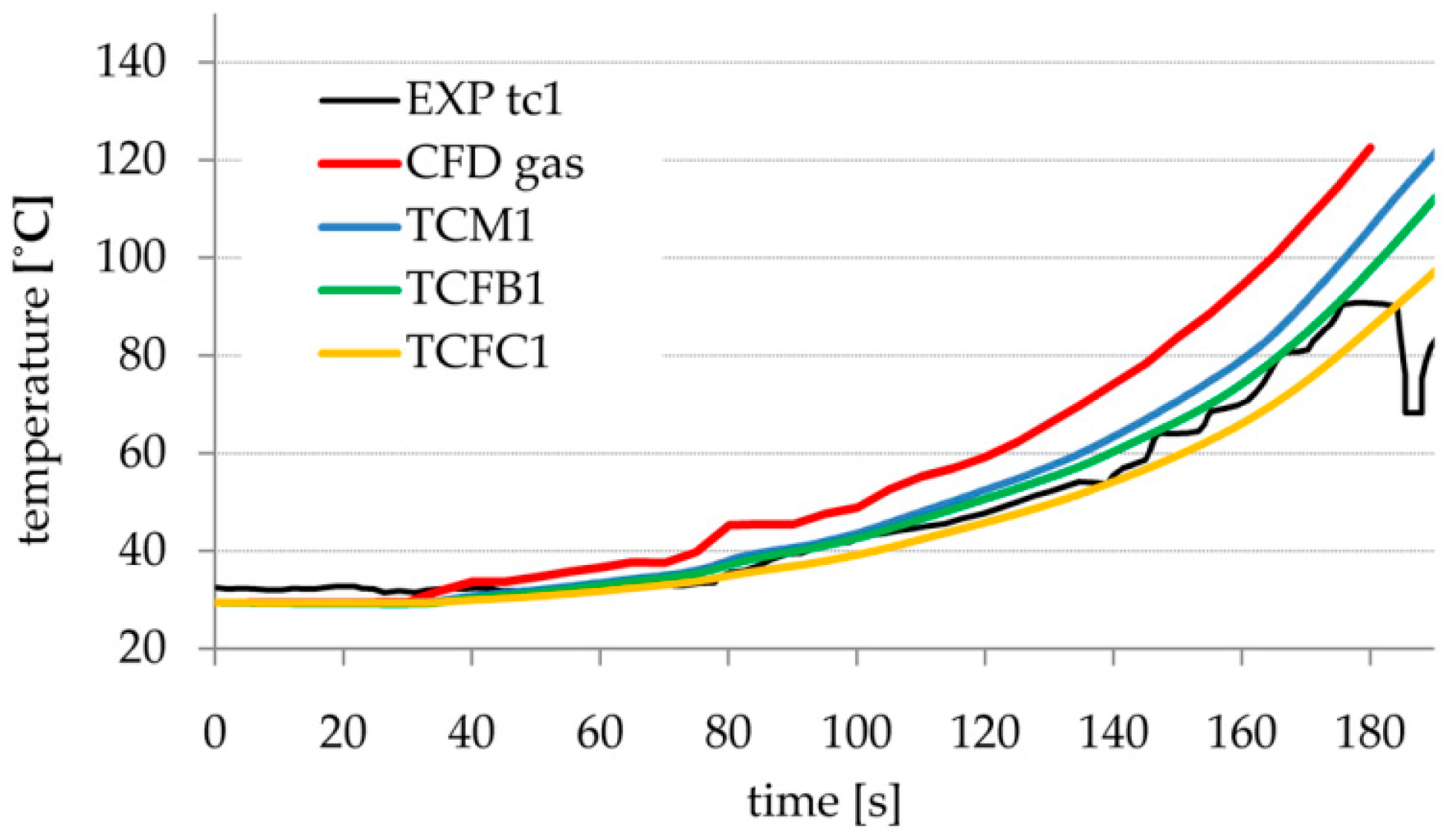
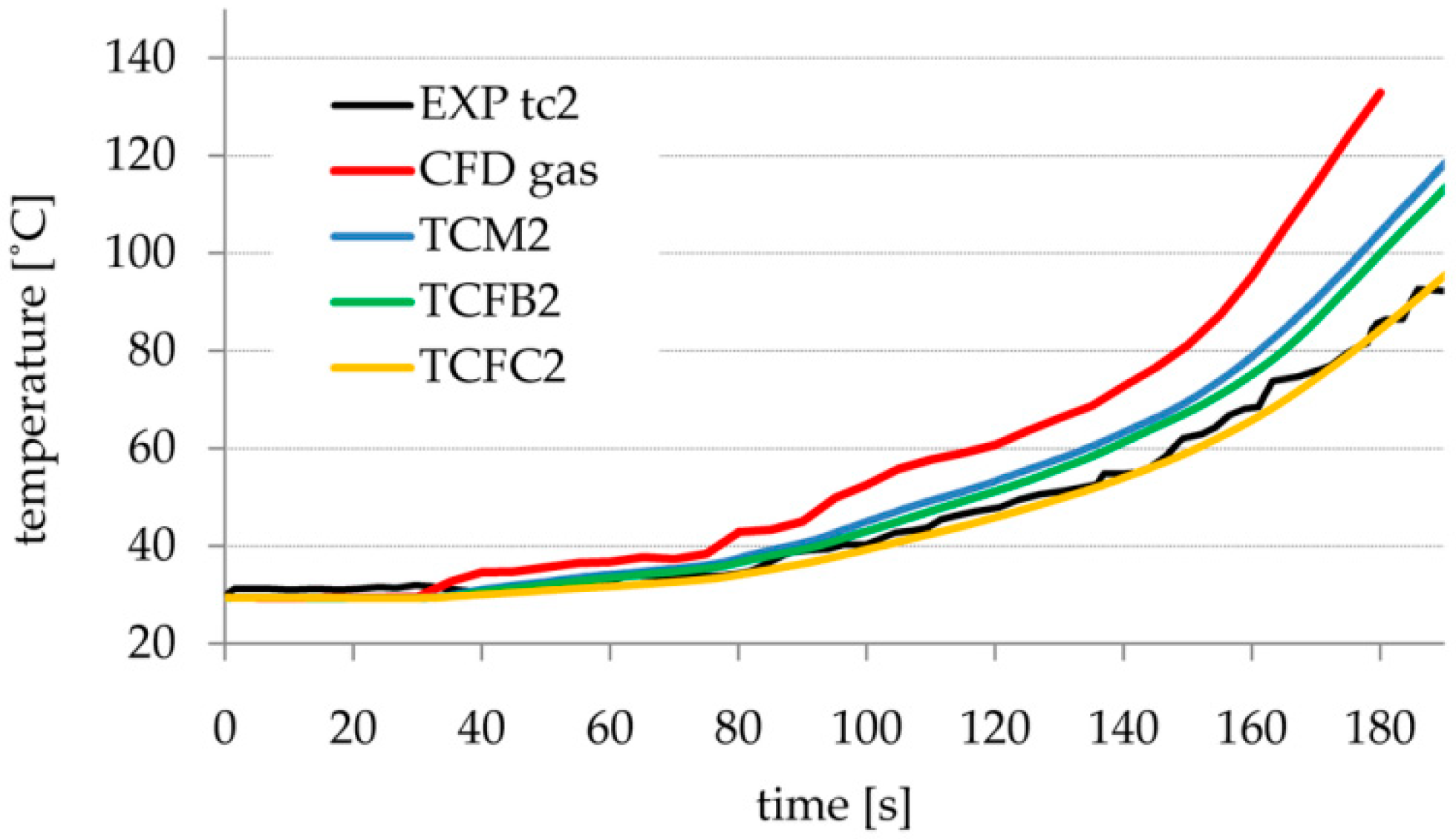
3.4.2. Results of Thermocouples Modeling
Thermocouples TC1 and TC2 (as in
Figure 1) are examined here. The results for experiment #10 are shown in
Figure 11 and
Figure 12. The series denoted as ‘EXP tcx’ presents data from measurements [
18,
19]. The series denoted as ‘CFD gas’ presents calculated fluid temperature at the thermocouples locations. The series denoted as TCFBx and TCFCx corresponds to the temperature of the physically modeled thermocouples of ball-shaped and cylindrical heads, respectively. The characteristic head diameter was 4 mm for both heads. Series TCMx contains the results of analytical thermocouple modeling (according to Equation (2)). All details linked to measurements of electric voltage are neglected here.
As can be easily observed, the calculated fluid temperature is significantly higher than the experimentally measured one. However, the results obtained for different models of thermocouples are much closer to the experimental data. This is due to fundamental differences between the real gas temperature and the measured temperature. The highest compliance was achieved for the physical models: the ball-shaped head for TC1 and cylindrical head for TC2. The results calculated with the analytical approach are close to those for the physical ball-shaped head, but a slightly higher temperature was always found. However, having in mind the earlier mentioned advantages of this approach it seems to be worth recommending.
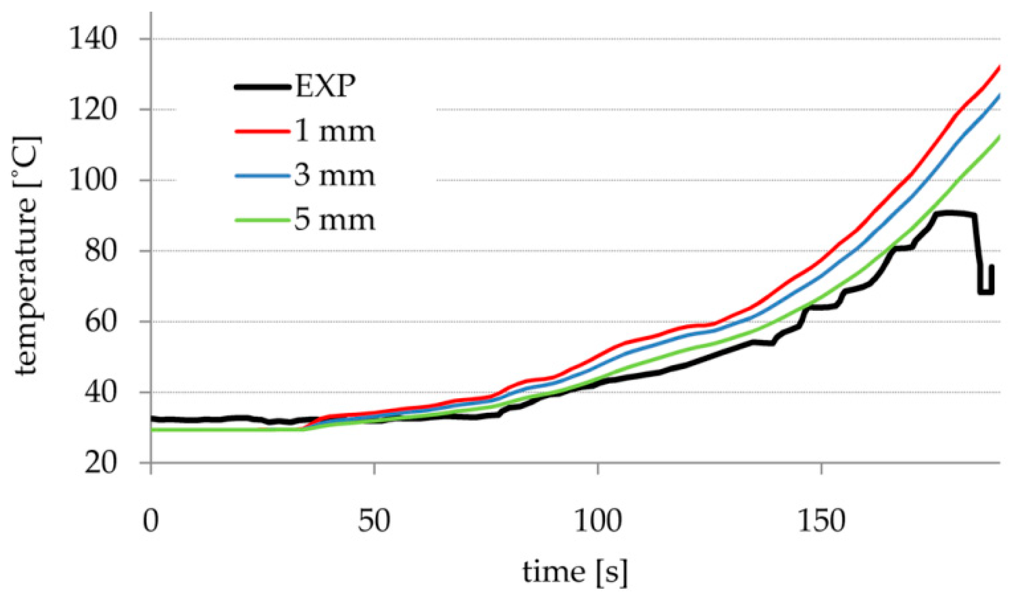
Since, according to Equations (1)–(4), the heat transfer rate depends in some degree on the characteristic dimension of a thermocouple head, this relation was examined numerically. Taking advantage of the proposed approach, a number of thermocouple heads of different characteristic dimensions were tested simultaneously. The results are presented in
Figure 13.
The important observation is that the results of thermocouple modeling are prone to the adopted head diameter. As the analytical model took into account, the thermal properties of a thermocouple head, termed the ‘’characteristic diameter’’, concern both the thermocouple head itself and the sheath if present.
3.4.3. Discussion
Although the presented results are generally in accordance with the measured values, some significant discrepancies can be observed. Both CFD (Fluent and FDS) results matched the real data quite well for the fire source located in the middle of the room. The simulations’ accuracy is much worse for the corner fire location, it concerns, especially, the FDS results. FDS predicted generally much longer sprinkler activation times or sprinklers were not activated at all during the simulations. Reasons of such variances are manifold, it is obvious that imperfections of numerical modeling play a predominant role here. The carried out comparison may lead to the conclusion that the LES turbulence model implemented in the FDS copes worse than the RSM model when applied to a complex flow structure. However, the nature of fire experiments also results in limited repeatability, which adds to the overall uncertainty. As was shown earlier, significant irregularities were already present at the input data stage (
Figure 7 and
Figure 8). The experimentally measured values of gas temperature showed clear fluctuations as well. All the above may cause the input parameters to be defined [
39] with some uncertainty and finally, in the light of such limitations, one can assess the achieved accuracy of the numerical modeling of sprinklers activation time and the temperature measurement process as satisfactory.
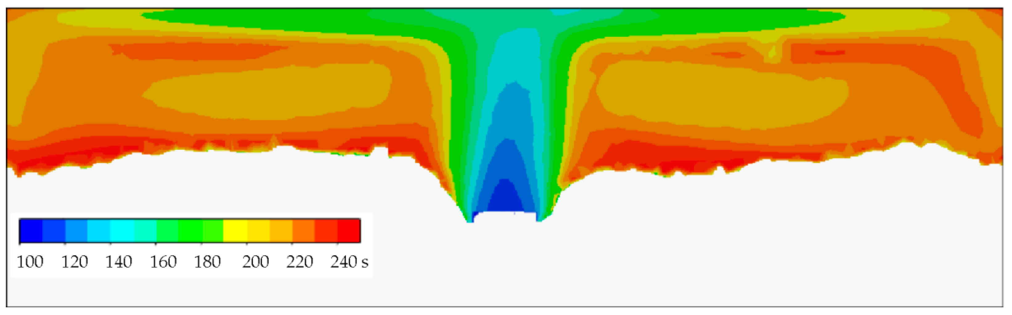
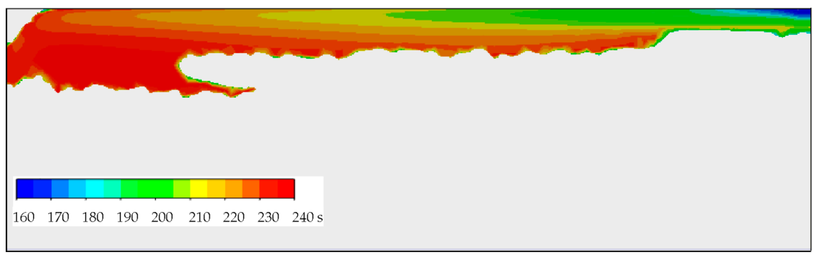
As was mentioned before, the main feature of the proposed approach is the possibility of placing virtual devices in each cell of the computational domain. This is an important novelty, even though the theoretical models applied for the sprinkler head and thermocouple modeling are already well recognized. This advantage allows for 2D or 3D visualizations of the calculated data in the same way as any flow field variables can be proceeded. These benefits are available for all researchers and practitioners, who are familiar with advanced features of ANSYS Fluent. These new opportunities allow for comprehensive visualization of the important properties of examined heat sensors in the whole computational domain instead of retrieving data point by point, which has been done so far. As an example, two maps of sprinklers activation time are presented in
Figure 14 (experiment #3) and
Figure 15 (experiment #17). The vertical plane of cross-section defined by SPR1 and SPR2 sprinkler positions (as in
Figure 1) is selected for visualization. Locations in which sprinklers would not have been activated at all during the simulation time are marked grey.
According to
Table 1 and
Table 2 the activation temperature of sprinklers used in these experiments was 68 °C. The results suggest that sprinklers should be mounted to position the device head in a thin layer of about 0.15 m under a firm ceiling. Significant temperature gradients can be observed in this layer, which may cause a high sensitivity of the activation time on the vertical location of a sprinkler head.
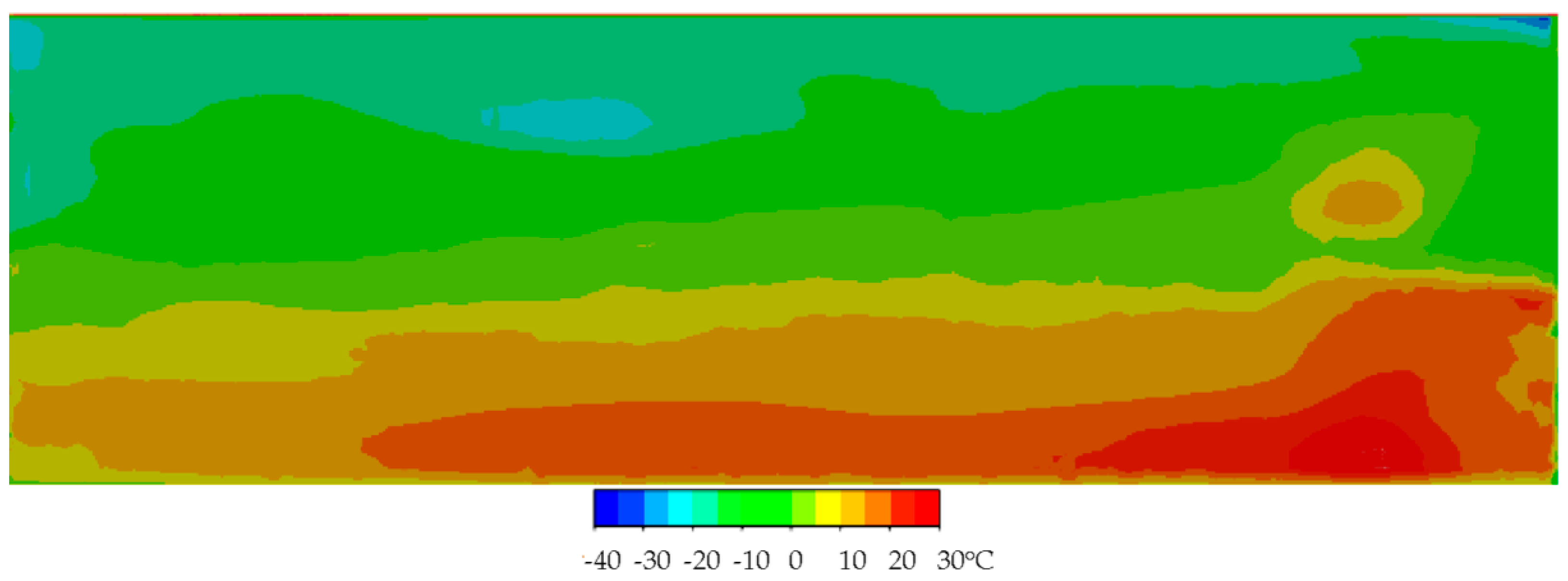
Figure 16 and
Figure 17 present the distribution of difference between the temperature measured by virtual thermocouples (of 2 mm diameter) and the calculated actual gas temperature for the same cross-section as previously.
In both cases presented large temperature deviations are observed. The temperature measured by a thermocouple can be either higher or lower than the real gas temperature, but the negative divergences are larger than the positive ones. The negative divergences are noticed in the upper parts of the compartment. This volume is filled by hot combustion gases, which strongly absorb radiation. Therefore the heat to a thermocouple bead is transferred directly from nearby portions of gas. When a fire is still developing, under conditions of imbalance, the bead temperature increase does not keep up with the surrounding gas temperature. This phenomenon is especially visible in the plume just above the fire. The positive divergences occur in the lower parts of the compartment, where the share of combustion products, including soot, are relatively low. This results in low optical density of the gas, and radiation is thus not absorbed intensively. Eventually, a thermocouple bead is heated by radiation and can reach a higher temperature than the surrounding gas.
4. Conclusions
This work presents the validation of the alternative approach to modeling of sprinklers and thermocouples. An important advantage of the proposed idea is that it tracks the processes in the heads of both devices as if they were placed in any cell of the computational domain. As such, there is no need to design the exact locations for them in advance, when planning the simulation. After the calculation is finished, one can retrieve data for any cell in the domain or prepare 2D or 3D maps of suitable variables. Furthermore, the same analysis can be simultaneously performed for multiple sprinkler types and thermocouple bead dimensions without any significant increase in the computational cost, as shown in [
11]. This can be used by the designers of sprinkler systems. They can quickly and easily design the arrangement of sprinklers in the building and choose the optimal type of sprinkler. It is the main advantage compared to other approaches, where sprinklers’ behavior is examined just in few predefined locations (e.g., FDS).
The data available in the literature were used for both model validations. The data came from real fire experiments, consisting of a series of 22 controlled compartment fires. In each fire, the course of fire development was monitored and recorded. Due to the significant observed fluctuations, these data showed the unpredictable nature of even controlled fire. Despite such fluctuated input data, the achieved results are in good accordance with the reported ones. However, one must be aware that real, and therefore modeled, fires may develop in an unrepeatable way. Hence, the presented approach makes decisions on selecting the most suitable sprinklers’ type and location easier. All considered cases were also examined using well known FDS software and the results were compared. While the results for cases with a central fire source location were generally in accordance and matched the experimental data, for cases with a corner fire location, FDS provided significantly overestimated times of sprinklers activation or even sprinklers were not activated at all. This is probably caused by the less accurate modeling of the hot gas flow under the ceiling due to the turbulence model applied (LES) and the lack of the inflation layers under the ceiling. This conclusion is of great practical importance, having in mind the wide range of this software use by practitioners dealing with fire protection of buildings.
The detailed analysis of the temperature measurement process by a thermocouple shows the significant divergences between the measured temperature and the actual one. This phenomenon occurs under conditions of imbalance, which are characteristic for quickly developing fire. The observed divergences were, at least, in the order of several dozen degrees and should be taken into account for accurate considerations. This observation may be very important for researchers who deal with experiments under real fire conditions.
Another important conclusion is the need of carefully choosing of the turbulence model to be used. The
k-ε and
k-ω turbulence models, which are commonly regarded as industry standards [
40,
41,
42,
43,
44], may fail when used for fire modeling in a confined space. This is due to expected anisotropy of flows, high velocity gradients and the essential role of buoyancy forces. The RSM model offers a suitable alternative in such circumstances.
The outcomes of the work might be of significant importance for practitioners, who deal with the issues of compartment fire modeling or building fire safety. The presented methods could help them to carry out multi-variant analyses in relatively low time consuming manner.

 ,
, 


