
Seismic Vulnerability Assessment of Portuguese Adobe Buildings


Abstract
1. Introduction
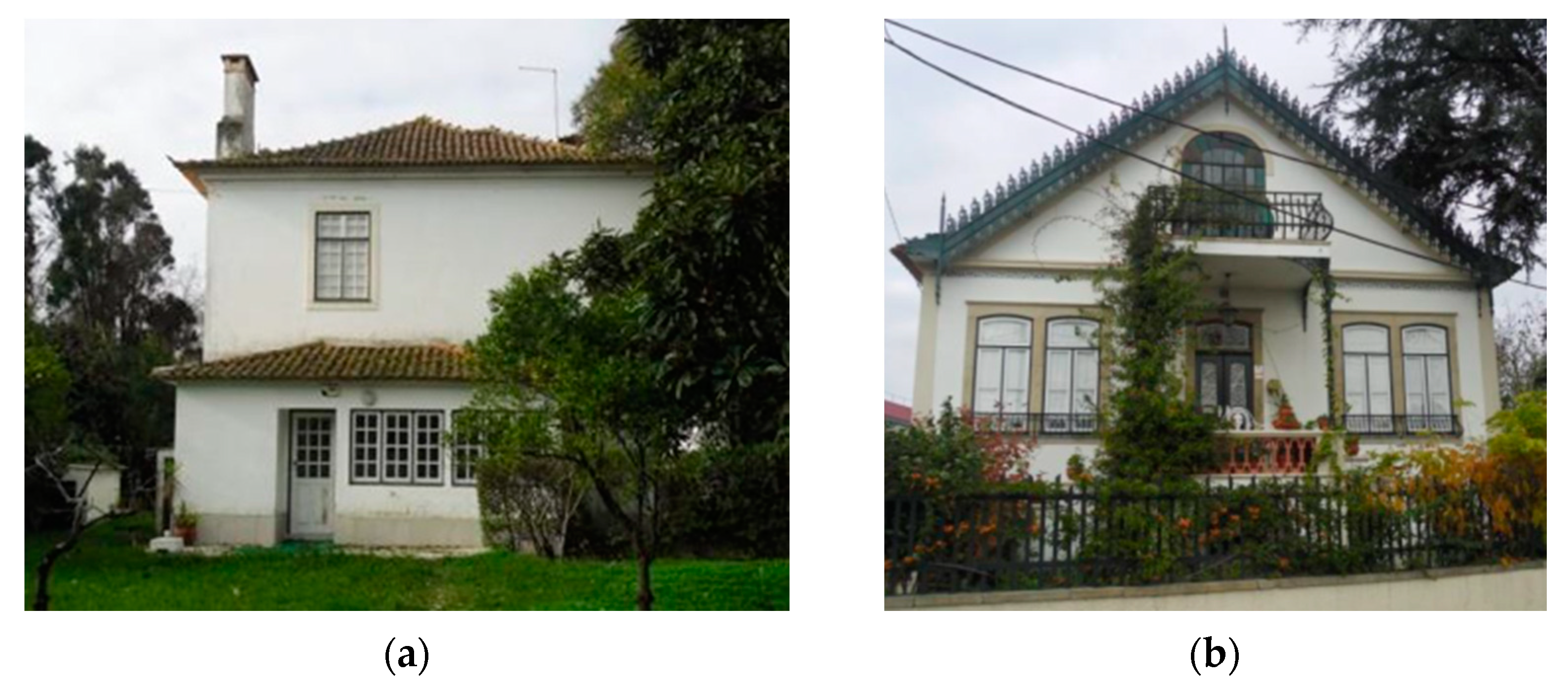
- Building surveys that contained well-documented evidence such as building schematics and descriptions of the buildings were examined. However, due to the scarcity of a large dataset specific to adobe buildings, three buildings with one archetype per building class of one-story, two-stories, and two-stories plus an attic were selected for the case study presented herein.
- These selected buildings were numerically modeled using the advanced finite element method-based software LS-DYNA [10]. These models were tested by following experimental validation and a series of sensitivity analyses to check the influence of various parameters.
- A set of 30 bi-directional ground motion records were selected based on the peak ground acceleration (PGA) as the intensity measure (IM), and used to perform several non-linear time-history analyses until the complete collapse of the buildings.
- To derive the fragility functions, two novel engineering demand parameters (EDPs)—namely the crack propagation ratio (CPR) and volume loss ratio (VLR)—were selected, and damage thresholds were proposed such that they can be correlated with the damage classifications of the European Macroseismic Scale (EMS-98) [11].
- The fragility functions were derived using the well-established cloud analysis [12] to quantify physical structural damage due to a given IM.
- Furthermore, a fatality vulnerability function was derived to estimate indoor fatalities.
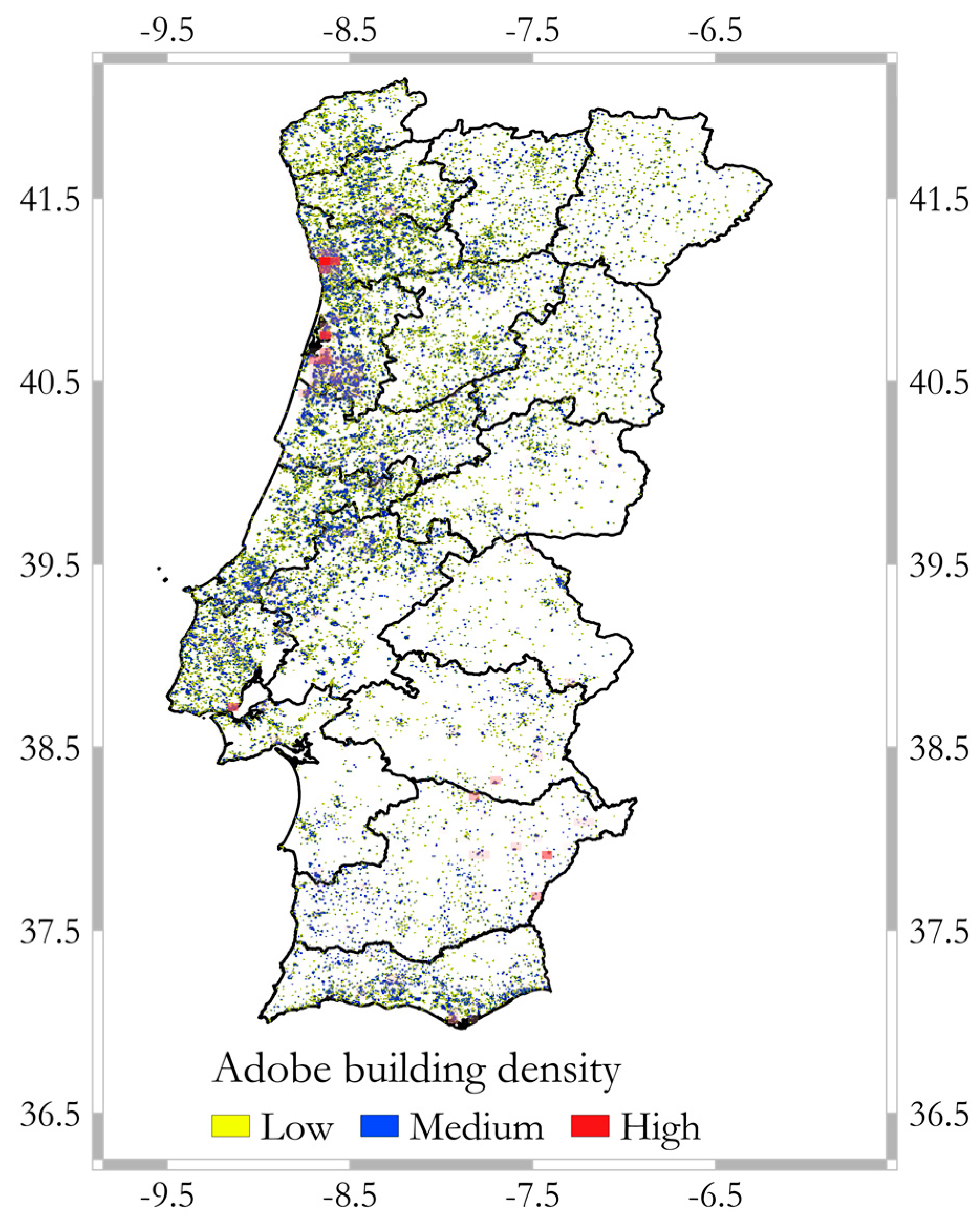
2. Characterization of Adobe Buildings in Portugal
Database of Adobe Buildings Information
3. Case Study Buildings—Geometrical and Material Properties
3.1. Geometrical Properties
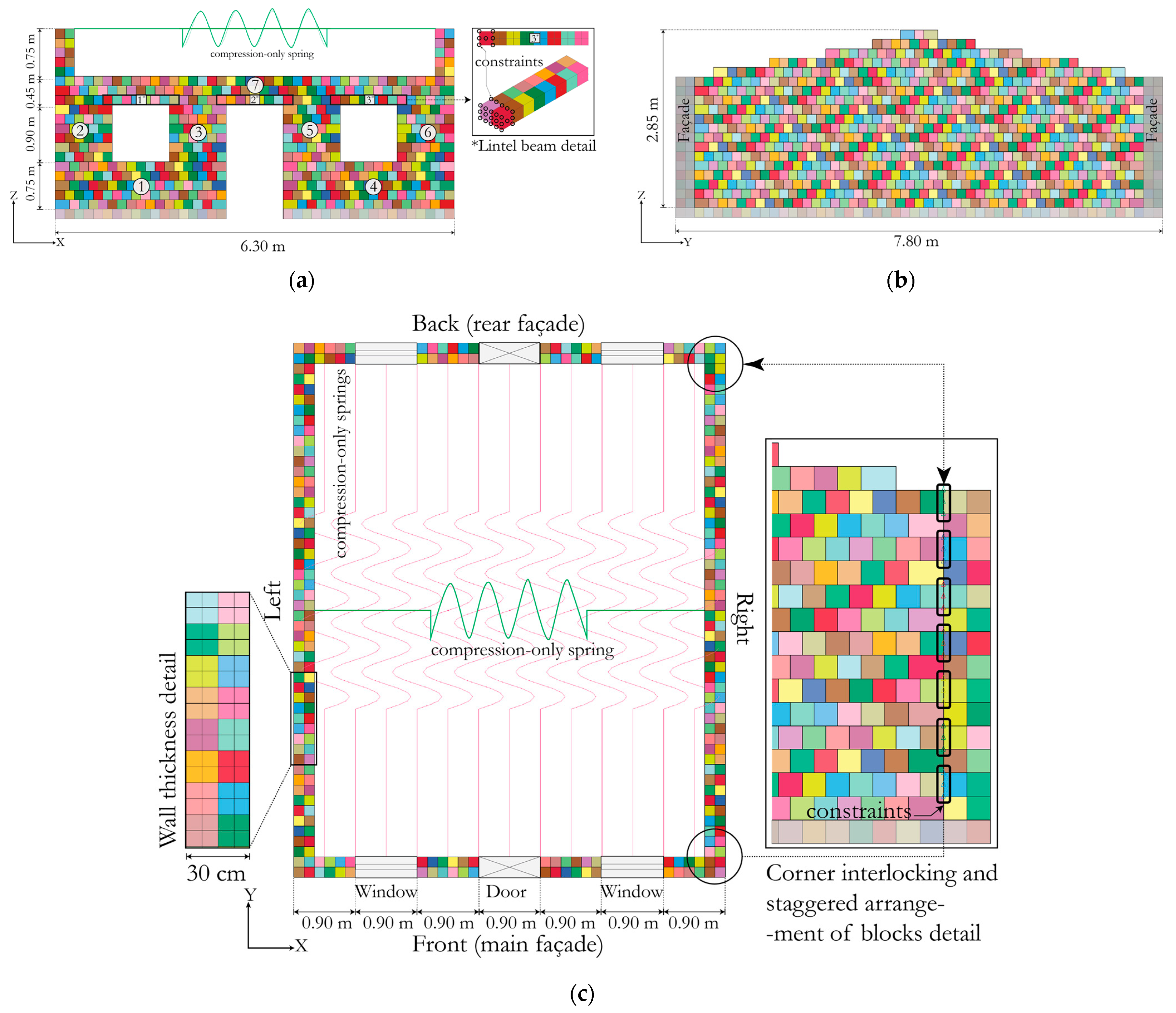
3.1.1. Building 1
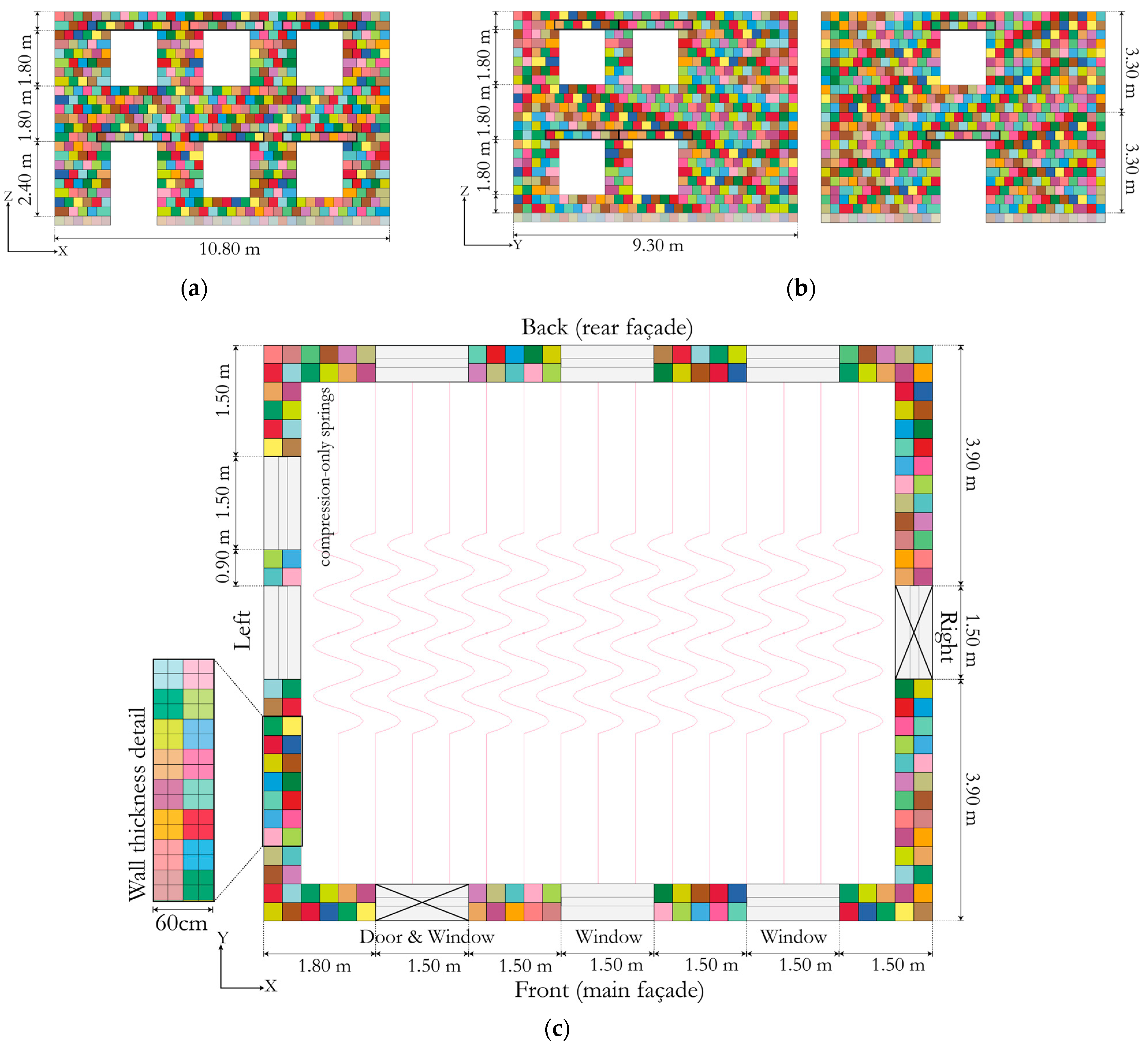
3.1.2. Building 2
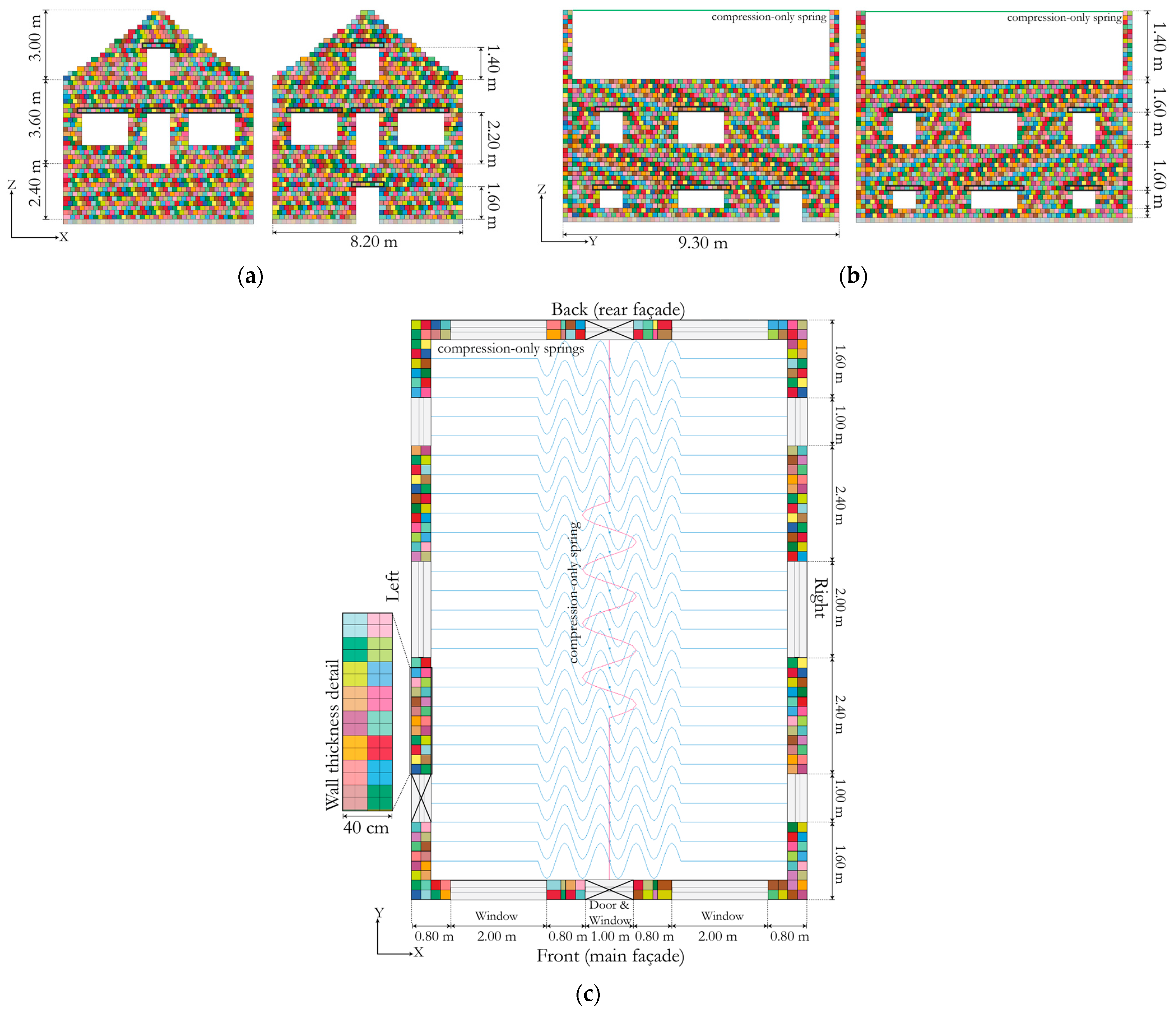
3.1.3. Building 3
3.2. Material Properties
3.2.1. Testing the Modeling Platform
3.2.2. Sensitivity Analysis
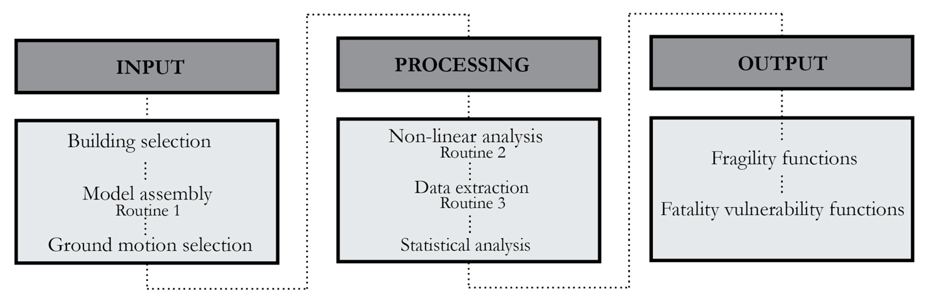
4. Framework for Vulnerability Assessment
4.1. Numerical Modeling
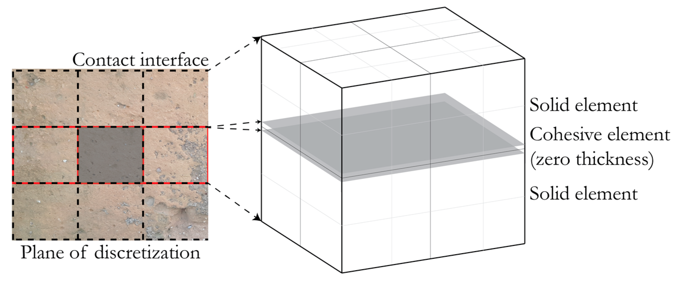
4.1.1. Solids Elements for Walls
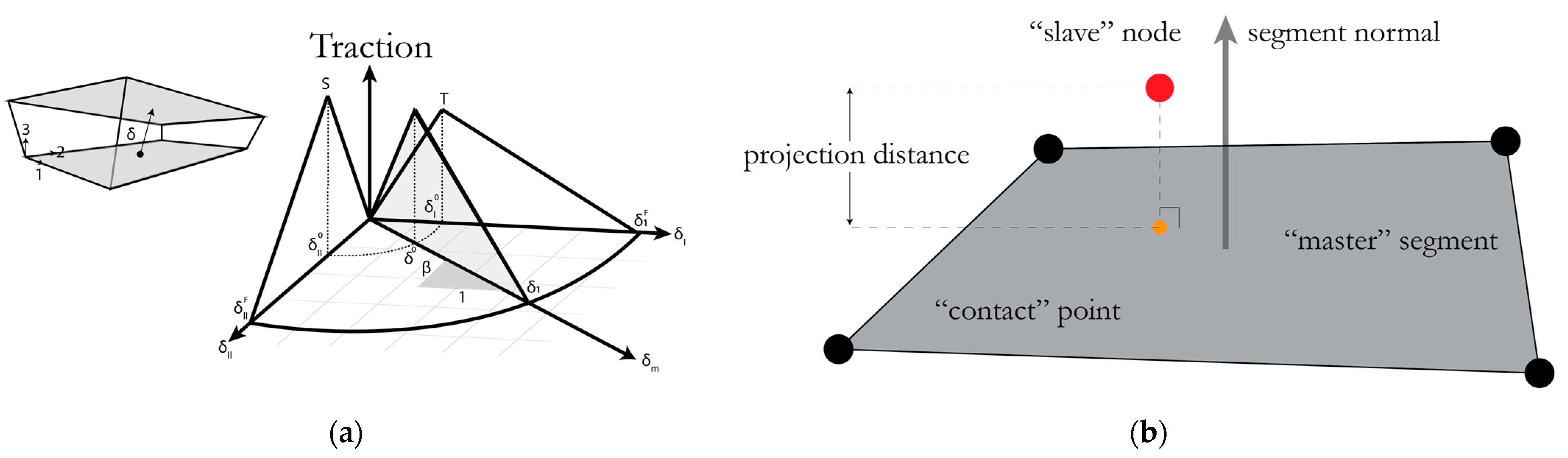
4.1.2. Segment Contact Interface Elements and Cohesive Mixed-Mode Material Model
4.1.3. Optimization
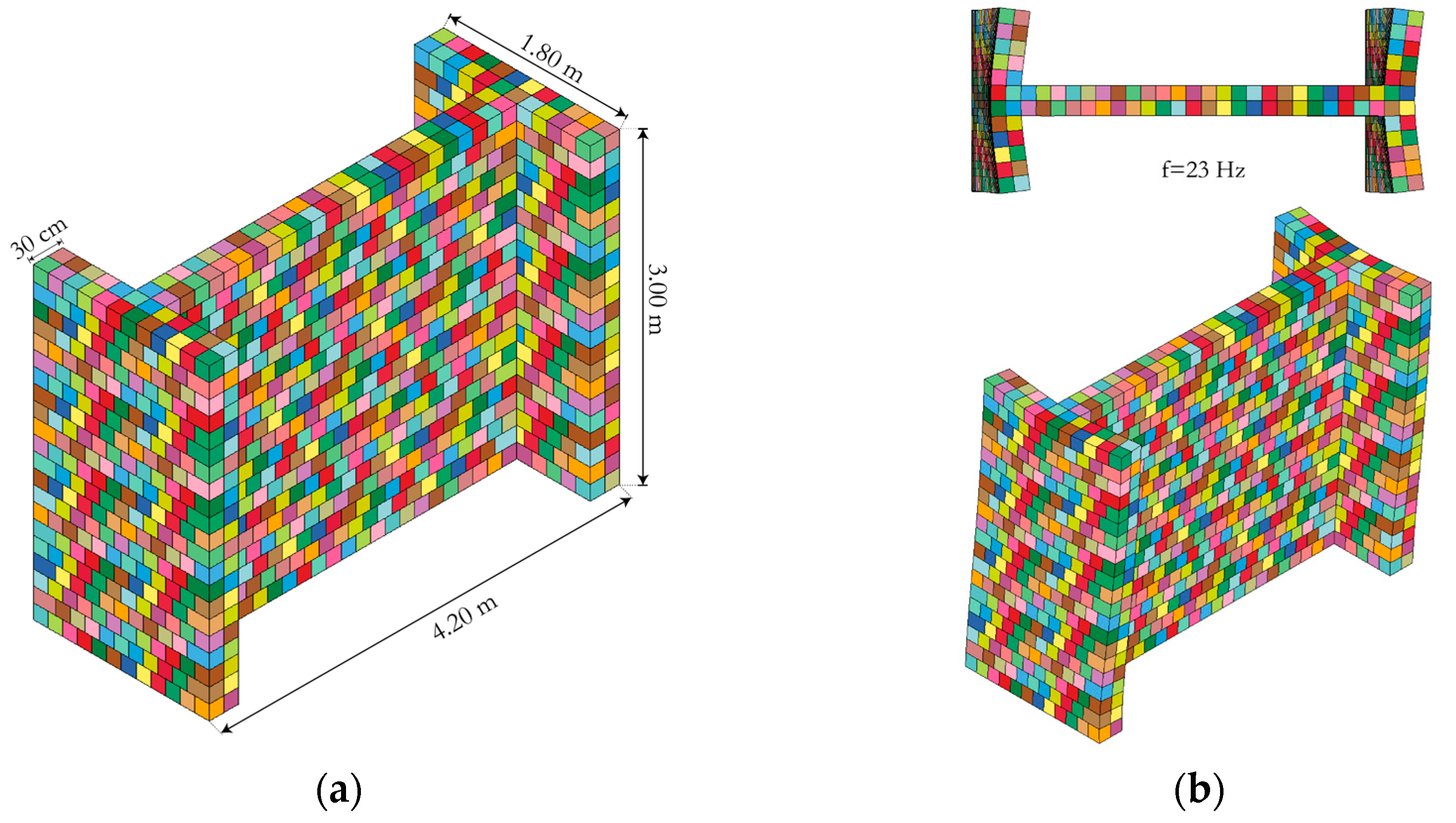
4.2. Eigenvalue Analysis
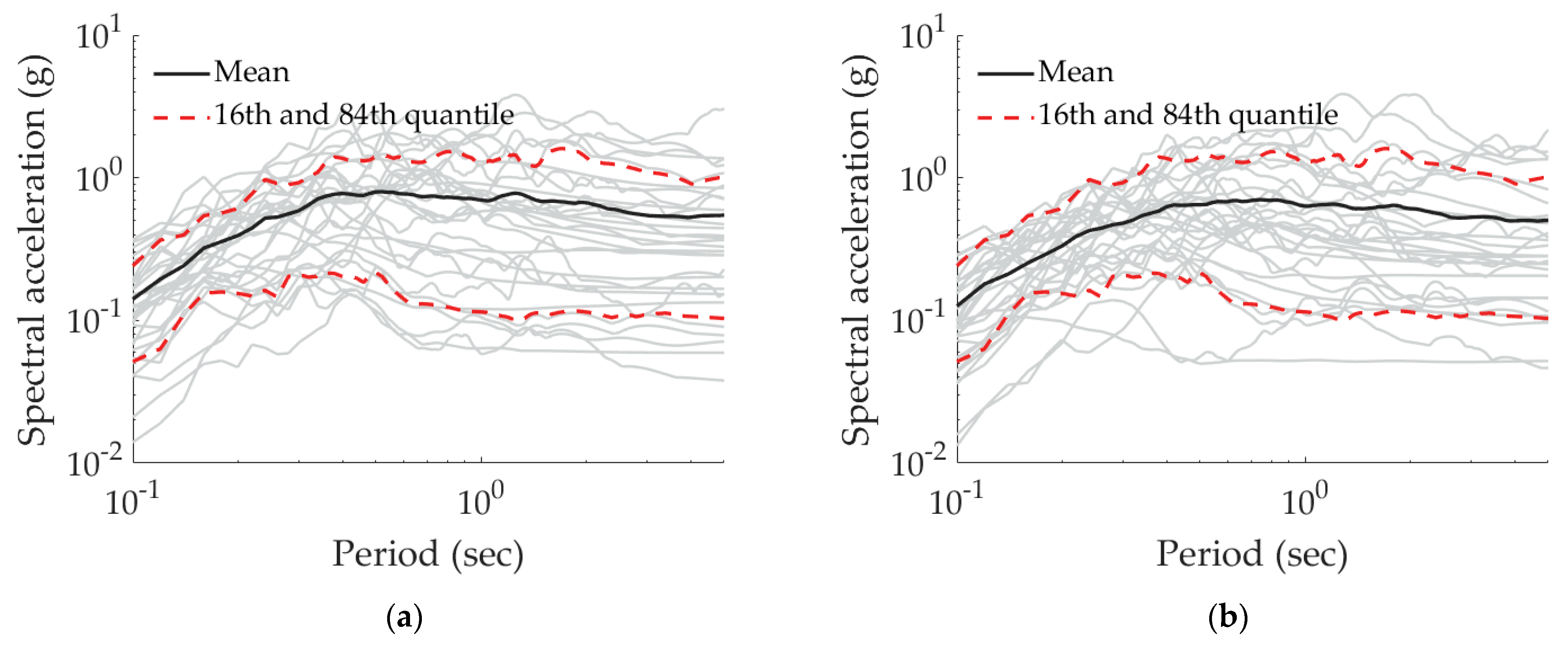
4.3. Hazard Demand
4.4. Non-Linear Time History Analysis
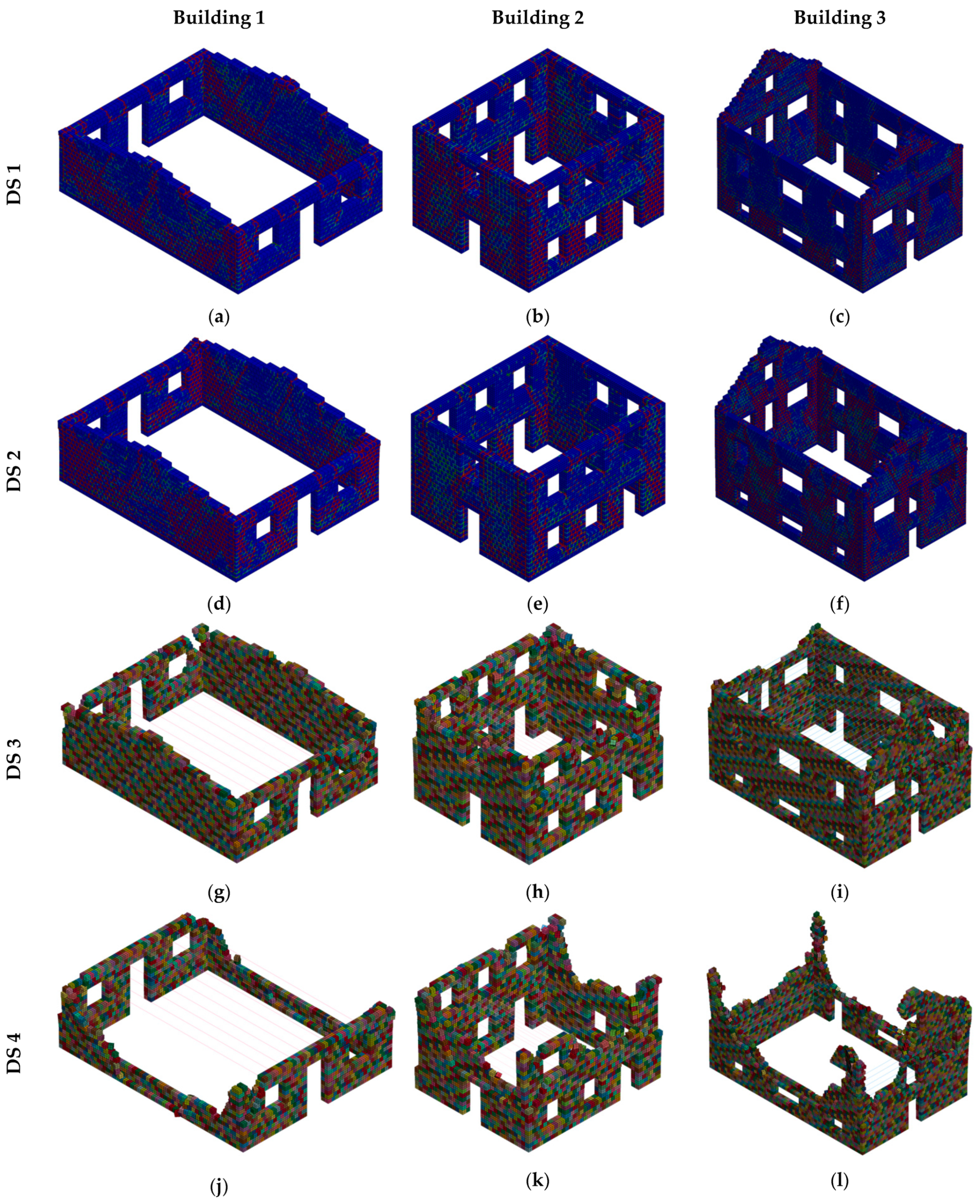
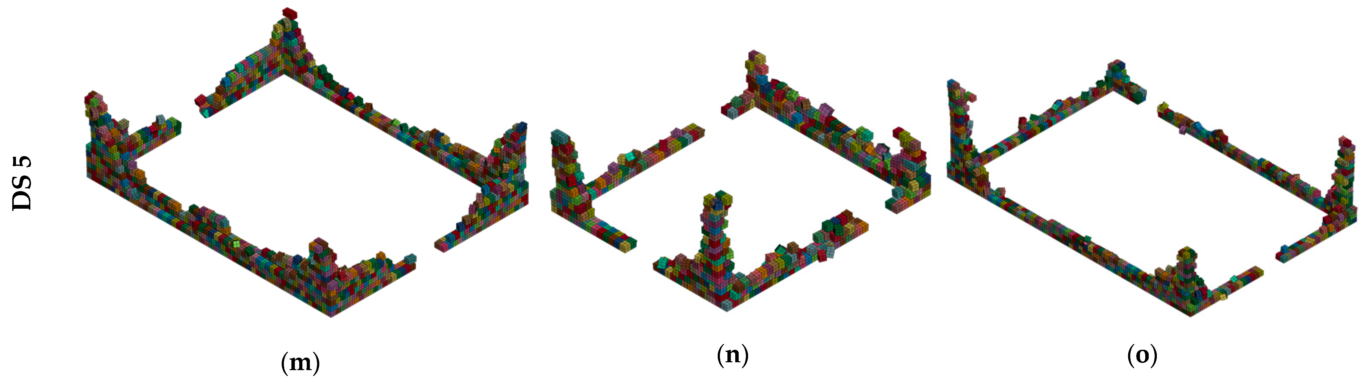
4.5. EDPs and DSs
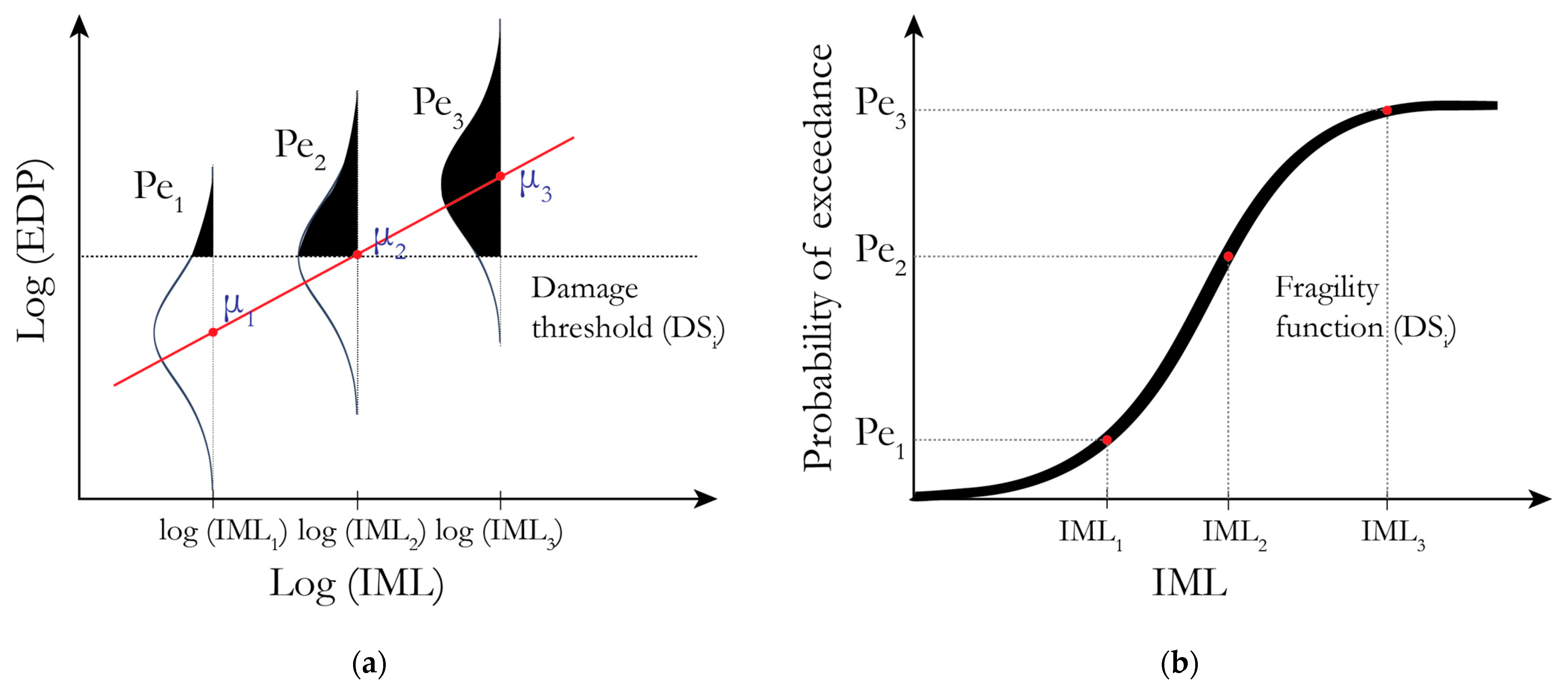
4.6. Cloud Analysis
- The results extracted from the non-linear time history analysis were plotted (IM vs. EDP) in a logarithmic scale, and a linear regression was performed to generate a trendline that best fits the data.
- The following equation was used to calculate the expected value of the dependent variable (EDP) given an IM. A homogeneity of variance was assumed for the IM-EDP random variables; hence the model can be described as shown in Equation (1).where stands for the expected logarithm of EDP given an IM, b and log(a) are the regression parameters, is the record-to-record variability, n is the no. of records, and corresponds to the i-EDP value obtained from the non-linear analysis for the corresponding .
- The structural fragility functions obtained from the probabilistic model can be expressed using Equation (2).where is the cumulative normal standard distribution and the is the damage threshold (e.g., 15%) corresponding to a given damage state (e.g., DS1).
4.7. Fatality Vulnerability Functions
5. Results
6. Conclusions
Author Contributions
Funding
Institutional Review Board Statement
Informed Consent Statement
Data Availability Statement
Conflicts of Interest
References
- Sousa, G.; Gallaecia, E.S. Historical Seismicity in Portugal. In Seismic Retrofitting: Learning from Vernacular Architecture; Taylor & Francis: Abingdon, UK, 2015. [Google Scholar]
- Choffat, P. Le tremblement de terre du 23 Avril 1909 dans le Ribatejo. In Revista de Obras Pu´blicas e Minas, Tomo XLIII; Imprensa Nacional: Lisboa, Spain, 1912. (In French) [Google Scholar]
- Tarque, N.; Crowley, H.; Pinho, R.; Varum, H. Displacement-Based Fragility Curves for Seismic Assessment of Adobe Buildings in Cusco, Peru. Earthq. Spectra 2012, 28, 759–794. [Google Scholar] [CrossRef]
- Crowley, H.; Pinho, R.; Bommer, J.J. A Probabilistic Displacement-based Vulnerability Assessment Procedure for Earthquake Loss Estimation. Bull. Earthq. Eng. 2004, 2, 173–219. [Google Scholar] [CrossRef]
- Ahmad, N.; Ali, Q.; Crowley, H.; Pinho, R. Earthquake loss estimation of residential buildings in Pakistan. Nat. Hazards 2014, 73, 1889–1955. [Google Scholar] [CrossRef]
- Villar-Vega, M.; Silva, V.; Crowley, H.; Yepes, C.; Tarque, N.; Acevedo, A.B.; Hube, M.A.; Gustavo, C.D.; María, H.S. Development of a Fragility Model for the Residential Building Stock in South America. Earthq. Spectra 2017, 33, 581–604. [Google Scholar] [CrossRef]
- Martins, L.; Silva, V. Development of a fragility and vulnerability model for global seismic risk analyses. Bull. Earthq. Eng. 2020, 2020, 1–27. [Google Scholar] [CrossRef]
- Sumerente, G.; Lovon, H.; Tarque, N.; Chácara, C. Assessment of Combined In-Plane and Out-of-Plane Fragility Functions for Adobe Masonry Buildings in the Peruvian Andes. Front. Built Environ. 2020, 6, 52. [Google Scholar] [CrossRef]
- Abeling, S.; Ingham, J.M. Volume loss fatality model for as-built and retrofitted clay brick unreinforced masonry buildings damaged in the 2010/11 Canterbury earthquakes. Structures 2020, 24, 940–954. [Google Scholar] [CrossRef]
- Hallquist, J.O. Livermore Software Technology Corporation (Lstc), Ls-Dyna Keyword User’s Manual Volume I; 2018; Volume II. Available online: https://ftp.lstc.com/anonymous/outgoing/jday/manuals/LS-DYNA_Manual_Volume_I_R11.pdf (accessed on 15 March 2021).
- Comisión Sismológica Europea. Escala Macro Sísmica Europea EMS-98; 1998; Volume 15. Available online: http://media.gfz-potsdam.de/gfz/sec26/resources/documents/PDF/EMS-98_Original_englisch.pdf (accessed on 15 March 2021).
- Jalayer, F.; De Risi, R.; Manfredi, G. Bayesian Cloud Analysis: Efficient structural fragility assessment using linear regression. Bull. Earthq. Eng. 2015, 13, 1183–1203. [Google Scholar] [CrossRef]
- De Estatística, I.N. Census Data 2011. Lisbon. 2011. Available online: http://censos.ine.pt/ (accessed on 15 March 2021).
- Costa, C.; Arduin, D.; Rocha, F.; Velosa, A. Adobe Blocks in the Center of Portugal: Main Characteristics. Int. J. Arch. Herit. 2019, 15, 467–478. [Google Scholar] [CrossRef]
- Correia, M.; Carlos, G.; Merten, J.; Viana, D.; Rocha, S. Vernacular Heritage and Earthen Architecture; Taylor & Francis Group: London, UK, 2013; pp. 111–116. [Google Scholar] [CrossRef]
- Varum, H.; Figueiredo, A.; Silveira, D.; Martins, T.; Costa, A. Investigaciones realizadas en la Universidad de Aveiro sobre caracterización mecánica de las construcciones existentes en adobe en Portugal y propuestas de rehabilitación y refuerzo. Resultados alcanzados. Inf. Constr. 2011, 63, 127–142. [Google Scholar] [CrossRef][Green Version]
- Varum, H.; Costa, A.; Fonseca, J.; Furtado, A. Behaviour Characterization and Rehabilitation of Adobe Construction. Procedia Eng. 2015, 114, 714–721. [Google Scholar] [CrossRef]
- Varum, H.; Costa, A.; Velosa, A.; Martins, T.; Pereira, H.; Almeida, J. Caracterização mecânica e patológica das construções em Adobe no distrito de Aveiro como suporte em intervenções de reabilitação. In Houses and Cities Built with Earth: Conservation, Significance and Urban Quality; CULTURA 2000—Education and Culture, European Union Program; ARGUMEMTUM: Monsaraz, Portugal, 2006; pp. 41–45. [Google Scholar]
- Silveira, D.; Varum, H.; Costa, A.; Neto, C. Survey of the Facade Walls of Existing Adobe Buildings. Int. J. Arch. Herit. 2016, 10, 867–886. [Google Scholar] [CrossRef][Green Version]
- IPQ. NP EN 1998-1. Eurocódigo 8: Projecto de Estruturas Para Resistência Aos Sismos. In Parte 1: Regras Gerais, Acções Sísmicas e Regras Para Edifícios; Instituto Português da Qualidade: Caparica, Portugal, 2010; p. 230. (In Portuguese) [Google Scholar]
- Braga, A.M.; Estêvão, J.M.C. Os Sismos E a Construção Em Taipa No Algarve. In Sísmica 2010–8° Congr. Sismol. e Eng. Sísmica; University of Aveiro: Aveiro, Portugal, 2010; pp. 1–13. [Google Scholar]
- Correia, M.R. Rammed Earth in Alentejo; Argumentum: Lisbon, Portugal, 2007. [Google Scholar]
- Cancela, D.C.P. Comportamento Higrotérmico e Monitorização de Construções em Adobe. Master’s Thesis, Civil Engineering, Univeristy of Aveiro, Aveiro, Portugal, 2013. [Google Scholar]
- EN 1995-1-2:2004. Part 1–2: General—Structural fire design. In Eurocode 5: Design of Timber Structures; CEN: Brussels, Belgium, 2004. [Google Scholar]
- Battaglia, L.; Ferreira, T.M.; Lourenço, P.B. Seismic fragility assessment of masonry building aggregates: A case study in the old city Centre of Seixal, Portugal. Earthq. Eng. Struct. Dyn. 2021, 50, 1358–1377. [Google Scholar] [CrossRef]
- Silveira, D.; Varum, H.; Costa, A.; Martins, T.; Pereira, H.; Almeida, J. Mechanical properties of adobe bricks in ancient constructions. Constr. Build. Mater. 2012, 28, 36–44. [Google Scholar] [CrossRef]
- Silveira, D.; Varum, H.; Costa, A. Influence of the testing procedures in the mechanical characterization of adobe bricks. Constr. Build. Mater. 2013, 40, 719–728. [Google Scholar] [CrossRef]
- Silveira, D.; Varum, H.; Costa, A.; Pereira, H.; Sarchi, L.; Monteiro, R. Seismic behavior of two Portuguese adobe buildings: Part I—in-plane cyclic testing of a full-scale adobe wall. Int. J. Arch. Herit. 2018, 12, 922–935. [Google Scholar] [CrossRef]
- Sarchi, L.; Varum, H.; Monteiro, R.; Silveira, D. Seismic behavior of two Portuguese adobe buildings: Part II—numerical modeling and fragility assessment. Int. J. Arch. Herit. 2018, 12, 936–950. [Google Scholar] [CrossRef]
- NIKER. New Integrated Knowledge Based Approaches to the Protection of Cultural Heritage from Earthquake-Induced Risk; Research Report; University of Padova: Padova, Italy, 2010. [Google Scholar]
- Karanikoloudis, G.; Lourenço, P.B. Structural assessment and seismic vulnerability of earthen historic structures. Application of sophisticated numerical and simple analytical models. Eng. Struct. 2018, 160, 488–509. [Google Scholar] [CrossRef]
- Ginell, W.S.; Tolles, E.L. Seismic Stabilization of Historic Adobe Structures. J. Am. Inst. Conserv. 2000, 39, 147–163. [Google Scholar] [CrossRef]
- Vargas, J.; Bariola, J.; Blondet, M.; Mehta, P.K. Seismic strength of adobe masonry. Mater. Struct. 1986, 19, 253–258. [Google Scholar] [CrossRef]
- Blondet, M.; Ginocchio, F.; Marsh, C.; Ottazzi, G.; Villa-Garcia, G.; Yep, J. Shaking Table Test of Improved Adobe Masonry Houses. In Proceedings of the 9th World Conference on Earthquake Engineering, Kyoto, Tokyo, Japan, 2–6 August 1988. [Google Scholar]
- Illampas, R.; Ioannou, I.; Charmpis, D.C. Adobe bricks under compression: Experimental investigation and derivation of stress–strain equation. Constr. Build. Mater. 2014, 53, 83–90. [Google Scholar] [CrossRef]
- Lourenço, P.B.; Pereira, J.M. Seismic Retrofitting Project Recommendations for Advanced Modeling of Historic Earthen Sites; Getty Conservation Institute: Los Angeles, CA, USA; TecMinho–University of Minho: Guimarães, Portugal, 2018. [Google Scholar]
- Alshawa, O.; Sorrentino, L.; Liberatore, D. Simulation Of Shake Table Tests on Out-of-Plane Masonry Buildings. Part (II): Combined Finite-Discrete Elements. Int. J. Arch. Herit. 2016, 11, 1–15. [Google Scholar] [CrossRef]
- Hazay, M.; Munjiza, A. Introduction to the Combined Finite-Discrete Element Method. In Computational Modeling of Masonry Structures Using the Discrete Element Method; IGI Global: Hershey, PA, USA, 2016; pp. 123–145. ISBN 1522502319. [Google Scholar]
- Dis, C. LS-DYNA/LS-PrePost Ex. 0. Introduction 2011, 31 (Suppl. S1), 1–74. [Google Scholar]
- T.M. Inc. MATLAB; T.M. Inc.: Natick, MA, USA, 2018. [Google Scholar]
- D’Altri, A.M.; Sarhosis, V.; Milani, G.; Rots, J.; Cattari, S.; Lagomarsino, S.; Sacco, E.; Tralli, A.; Castellazzi, G.; De Miranda, S. Modeling Strategies for the Computational Analysis of Unreinforced Masonry Structures: Review and Classification. Arch. Comput. Methods Eng. 2020, 27, 1153–1185. [Google Scholar] [CrossRef]
- Pulatsu, B.; Erdogmus, E.; Lourenço, P.B.; Lemos, J.V.; Tuncay, K. Simulation of the in-plane structural behavior of unreinforced masonry walls and buildings using DEM. Structure 2020, 27, 2274–2287. [Google Scholar] [CrossRef]
- Bala, S. Tie-Break Contacts in LS-DYNA; Livemore Software: Livermore, CA, USA, 2007. [Google Scholar]
- Sousa, L.; Marques, M.; Silva, V.; Varum, H. Hazard Disaggregation and Record Selection for Fragility Analysis and Earthquake Loss Estimation. Earthq. Spectra 2017, 33, 529–549. [Google Scholar] [CrossRef]
- Hallquist, J.O. LS Dyna Theory Manual; Livemore Software: Livermore, CA, USA, 2006. [Google Scholar]
- Costa, A.; Humberto, V.; João, M.G. Structural Rehabilitation of Old Buildings; Springer: Berlin/Heidelberg, Germany, 2014. [Google Scholar]
- Pomonis, A. Derivation of Globally Applicable Casualty Rates for use in Earthquake Loss Estimation Models. In Proceedings of the 15th World Conference Earthquake Engineering, Lisbon, Portugal, 24–28 September 2012. [Google Scholar]
- Vamvatsikos, D.; Cornell, C.A. Incremental dynamic analysis. Earthq. Eng. Struct. Dyn. 2002, 31, 491–514. [Google Scholar] [CrossRef]
- Vamvatsikos, D.; Cornell, C.A. Direct Estimation of Seismic Demand and Capacity of Multidegree-of-Freedom Systems through Incremental Dynamic Analysis of Single Degree of Freedom Approximation. J. Struct. Eng. 2005, 131, 589–599. [Google Scholar] [CrossRef]
- Okada, S. Description for indoor space damage degree of building in earthquake. In Proceedings of the Eleventh World Conference on Earthquake Engineering, Acapulco, Mexico, 23–28 June 1996. [Google Scholar]


| Building Characteristics | Building 1 | Building 2 | Building 3 | |
|---|---|---|---|---|
| Total no. of stories | 1 | 2 | 2 + Attic | |
| Length (m) | X-direction | 6.30 | 10.80 | 8.20 |
| Y-direction | 7.80 | 9.30 | 12.00 | |
| Area (m2) | 49.14 | 100.44 | 98.40 | |
| Height (m) | 1st Story | 2.85 | 3.30 | 2.40 |
| 2nd Story | - | 3.30 | 3.60 | |
| Attic | - | - | 3.00 | |
| Total height (m) | 2.85 | 6.60 | 9.00 | |
| Total no. of external walls | 4 | 4 | 4 | |
| External wall thickness (cm) | 30 | 60 | 40 | |
| Gable-end walls | Yes | No | Yes | |
| Lintel beams | Yes | Yes | Yes | |
| Total no. of window openings | 4 | 15 | 16 | |
| Total no. of door openings | 2 | 3 | 4 | |
| Total percentage of openings (%) | 10 | 20 | 15 | |
| Element | Mechanical Properties | Value | Units |
|---|---|---|---|
| SOLID elements | Young’s modulus | 0.74 | GPa |
| Poison’s ratio | 0.30 | - | |
| Density | 1500 | kg/m3 | |
| Cohesive elements | Static coeff. of friction | 0.4 | - |
| Dynamic coeff. of friction | 0.3 | - | |
| Scale factor for segment penalty stiffness | 1.0 | - | |
| Normal and shear failure stress | 0.05 | MPa | |
| Normal and shear energy release rate | 10, 30, 20 | N/m | |
| Normal (CN) and tangential stiffness | 0.74 | GPa | |
| Springs | Timber elasticity modulus | 7.00 | GPa |
| Timber elasticity modulus (5%) | 4.70 | GPa | |
| Design compressive strength | 16.00 | MPa | |
| Design bending strength | 14.00 | MPa |
| Building 1 | Building 2 | Building 3 | |
|---|---|---|---|
| Mesh size (cm) | 7.5 | 15 | 10 |
| Block size (cm) | 15 | 30 | 20 |
| No. of nodes | 141,408 | 123,156 | 300,654 |
| No. of solid elements | 42,223 | 37,040 | 89,962 |
| No. of parts | 5162 | 4433 | 10,932 |
| Total volume of blocks composing the walls (m3) | 17.80 | 124.90 | 89.90 |
| Roof | Spring-based | Spring-based | Spring-based |
| EDPs | DSs | Damage Description | Threshold |
|---|---|---|---|
| Crack propagation ratio | DS 1 | Negligible to slight | 15% |
| DS 2 | Moderate | 25% | |
| Volume loss ratio | DS 3 | Substantial to heavy | 10% |
| DS 4 | Very heavy | 25% | |
| DS 5 | Destruction | 40% |
| Building Class | θ * | β ** |
|---|---|---|
| 1-story | 1.06 | 0.88 |
| 2-story | 0.45 | 0.75 |
| 2-story plus attic | 0.45 | 0.77 |
| Building Class | IM | DS 1 | DS 2 | DS 3 | DS 4 | DS 5 | |||||
|---|---|---|---|---|---|---|---|---|---|---|---|
| µ * | σ ** | µ | σ | µ | σ | µ | σ | µ | σ | ||
| 1-story | PGA | −0.89 | 0.39 | −0.67 | 0.39 | −0.43 | 0.37 | −0.20 | 0.37 | −0.08 | 0.37 |
| 2-story | PGA | −1.38 | 0.43 | −1.00 | 0.43 | −0.38 | 0.50 | −0.05 | 0.50 | 0.12 | 0.50 |
| 2-story plus attic | PGA | −1.39 | 0.42 | −0.96 | 0.42 | −0.46 | 0.49 | −0.17 | 0.49 | −0.02 | 0.49 |
Publisher’s Note: MDPI stays neutral with regard to jurisdictional claims in published maps and institutional affiliations. |
© 2021 by the authors. Licensee MDPI, Basel, Switzerland. This article is an open access article distributed under the terms and conditions of the Creative Commons Attribution (CC BY) license (https://creativecommons.org/licenses/by/4.0/).
Share and Cite
Momin, S.; Lovon, H.; Silva, V.; Ferreira, T.M.; Vicente, R. Seismic Vulnerability Assessment of Portuguese Adobe Buildings. Buildings 2021, 11, 200. https://doi.org/10.3390/buildings11050200
Momin S, Lovon H, Silva V, Ferreira TM, Vicente R. Seismic Vulnerability Assessment of Portuguese Adobe Buildings. Buildings. 2021; 11(5):200. https://doi.org/10.3390/buildings11050200
Chicago/Turabian StyleMomin, Samar, Holger Lovon, Vitor Silva, Tiago Miguel Ferreira, and Romeu Vicente. 2021. "Seismic Vulnerability Assessment of Portuguese Adobe Buildings" Buildings 11, no. 5: 200. https://doi.org/10.3390/buildings11050200
APA StyleMomin, S., Lovon, H., Silva, V., Ferreira, T. M., & Vicente, R. (2021). Seismic Vulnerability Assessment of Portuguese Adobe Buildings. Buildings, 11(5), 200. https://doi.org/10.3390/buildings11050200