The Effect of Atmospheric Corrosion on Steel Structures: A State-of-the-Art and Case-Study

Abstract

Atmospheric corrosion can seriously affect the performance of steel structures over long periods of time; thus, it is essential to evaluate the rate of corrosion and subsequent modification of dynamic properties of a structure over different time periods. Standards and codes represent the general guidelines and suggest general protection techniques to prevent structures from corrosion damage. The available models in the literature propose the thickness reduction method that accounts for the exposure time of structures in corrosive environments. The purpose of this study is to review the existing corrosion models in the literature and report as well as compare their effectiveness in low (C2 level), medium (C3 level) and high (C4 level) corrosivity class in accordance with the ISO standard. Furthermore, the influence of corrosion loss during the lifetime of a structure is studied through a realistic case study model using FEM (finite element method) in both linear and nonlinear regions. The results showed that the corrosion can considerably affect the dynamic characteristics of the structure. For instance, the vibration period rose up to 15% for the C4 class and 100-year lifespan. Additionally, the corroded structure presented higher acceleration and drift demand, and the base reaction forces were reduced up to 60% for the same class and time period.

1. Introduction

Structural steel tends to corrode naturally due to exposure to moisture and oxygen and the annual cost due to corrosion of steel structures, especially at coastal sites, can be tremendous. According to the last report of National Association of Corrosion Engineers (NACE), the global cost of corrosion was estimated about USD 2.5 trillion annually, which is 3.4% of the global gross domestic product (GPD) [1]. However, structural systems can be protected against corrosion and exhibit adequate lifetimes by employing appropriate maintenance techniques and rational design.

The effect of corrosion is defined by the average depth loss; D, relative to the initial thickness and mass loss ratio as follows:

$$D=\left(\frac{m_0-m}{m_0}\right) \ast t_0$$

(1)

where m and m₀ are the mass of corroded and uncorroded components in the same order and t₀ is the thickness of the undamaged element. Corrosion mass loss can reduce the overall structural performance by changing the inherent structural characteristics of the system.

Recently, a study [2] was conducted regarding the dynamic characteristics of two code-consistent steel truss structures with respect to corrosion propagation in marine environment. The results showed that the frequency was reduced for all modes of vibration and structures, considering maximum corrosion depth, D, equal to 1.4 mm. It is worth noticing that the first transversal mode of a truss roof was reduced by 17% which corresponded to the maximum D and 20 years of exposure.

Material mechanical properties are modified after severe corrosion attacks. Recently, some researchers focused on the efficacy of the corrosion loss on the physical properties and seismic performance of corroded components through tensile strength testing [3,4,5,6,7,8]. The value of material properties (yield and ultimate strength, module of elasticity and elongation) were declined with the growth of corrosion damage level. Additionally, [5] showed that a structure can experience a decrease in the amount of energy dissipation and an increase in the maximum story drift ratio when the mass loss increases.

There are a number of corrosion wastage models for steel structures which relate the effective environmental factors to the exposure over time [9,10,11]. Most of these models were calibrated in marine environments that have the highest rate of damage, and are impractical in other corrosive environments with different environmental conditions (different rates of sulfur, chloride ion or relative humidity). Indeed, there is scarce literature regarding the assessment of corrosion effects in urban and especially in industrial zones with medium rates of pollutants, whereas the European codes [12] provide general recommendations, mostly related to appropriate surface protection techniques and materials to prevent corrosion occurrence, but there are no guidelines on the evaluation of thickness loss with time.

The objective of the present study is to provide a comprehensive review of available corrosion models of steel structures in the literature and study their effectiveness in structural performance in different atmospheric environmental conditions in long-term of exposure, focusing on low to high (C2 to C4) corrosivity classes. These levels can be expressed by the presence of corrosive factors in air from rural atmosphere (low rate of pollutant) to industrial atmosphere (high rate of pollutant, see

Table 1. Different corrosivity categories based on ISO9223 [13].

Corrosivity Categories	Corrosivity	Typical Outdoor Atmospheric Environments
C1	Very low	Dry or cold zone with very low pollution and TOW * e.g., deserts, Antarctic zone
C2	Low	Temperate zone with low pollution (SO2 (μg/m3) < 5), e.g., rural areas.
		Dry and cold zone with short TOW, e.g., deserts and subarctic areas
C3	Medium	Temperate zone with medium pollution (5 < SO2 (μg/m3) < 30) and low chloride effect, e.g., urban areas and coastal areas with low concentration of chloride ions Subtropical and tropical zones with low pollution
C4	High	Temperate zone with high pollution (30 < SO2 (μg/m3) < 90) or considerable effect of chlorides, e.g., polluted urban areas, industrial areas, coastal areas without spray of salt water or, de-icing salts influences Subtropical and tropical zone with medium pollution
C5	Very high	Temperate zones with high pollution levels (90 < SO2 (μg/m3) < 250); high chloride deposition rates, e.g., industrial areas, coastal and sea zones and sheltered positions on coastline.
CX	Extreme	Subtropical and tropical zone with significant TOW, atmospheric environment with very high level of SO2 deposits (SO2 (μg/m3) > 250) including accompanying and production factors with profound effect of chloride concentration, e.g., extreme industrial areas, coastal areas and contact with salt spray

* TOW = time of wetness.

).

To fulfil this goal, first a holistic view of the mechanism of corrosion and its main causes in steel structures were provided. Then, a quantitative comparison of the most updated and reliable corrosion models of steel structures in atmospheric environment according to the various corrosivity categories (Table 1) are reported and the most significant differences in long period of time were outlined. Furthermore, to assess the dynamic characteristics of corroded structures, a realistic case study that refers to a process unit inside a petrochemical plant was analyzed using the finite element method (FEM) in various corrosion rates. Nonlinear time history analyses (NLTH) were carried out to evaluate the seismic response of the structure under earthquake records.

2. Corrosion of Metals

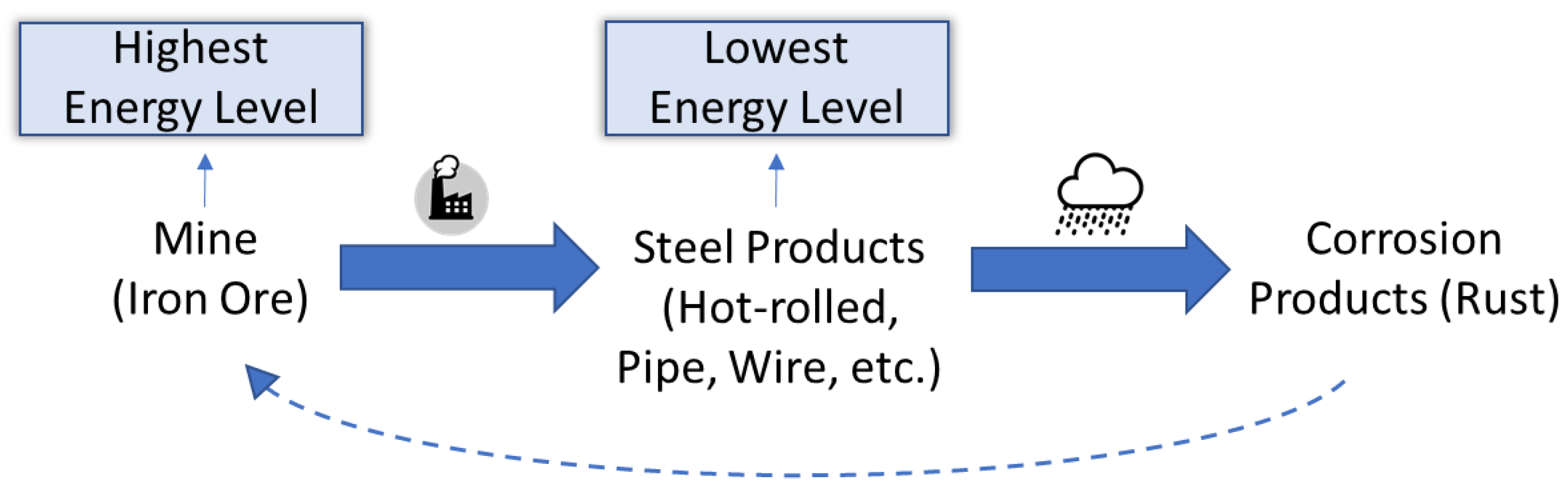
Metals are rarely in their elemental forms and they are combined with oxygen and other abundant chemicals to form thermodynamically stable ores. These tend to be oxides and mineral ores; hence, they are found in this form and must be purified in energy intensive processes (Figure 1). Corrosion is defined chemically as a spontaneous chemical or electrochemical reaction between a material (generally metal or alloy) and a corrosive environment that leads to destruction of material [14].

The chemical reactivity of a metal often involves the transfer of its electrons to environmental electron scavengers and an electrochemical process that tends to see the electrons move in order to complete an electrical circuit, which can occur when certain electrolyte solutions come in contact with the metals, either from moisture, soils or gasses. The difference of potential between two areas of the metal, named cathodic (reduction of hydrogen or oxygen ions) and anodic (oxidation or dissolution of the metal), can produce an electric current which can result in thickness loss on the entire surface or locally [14].

Corrosion can be classified using different approaches. The most conventional classification divides the corrosion types according to their appearance which some of them can be identified visually and others are not visible (Figure 2). The most common types of corrosion attacks on steel components can be expressed as follows [14]:

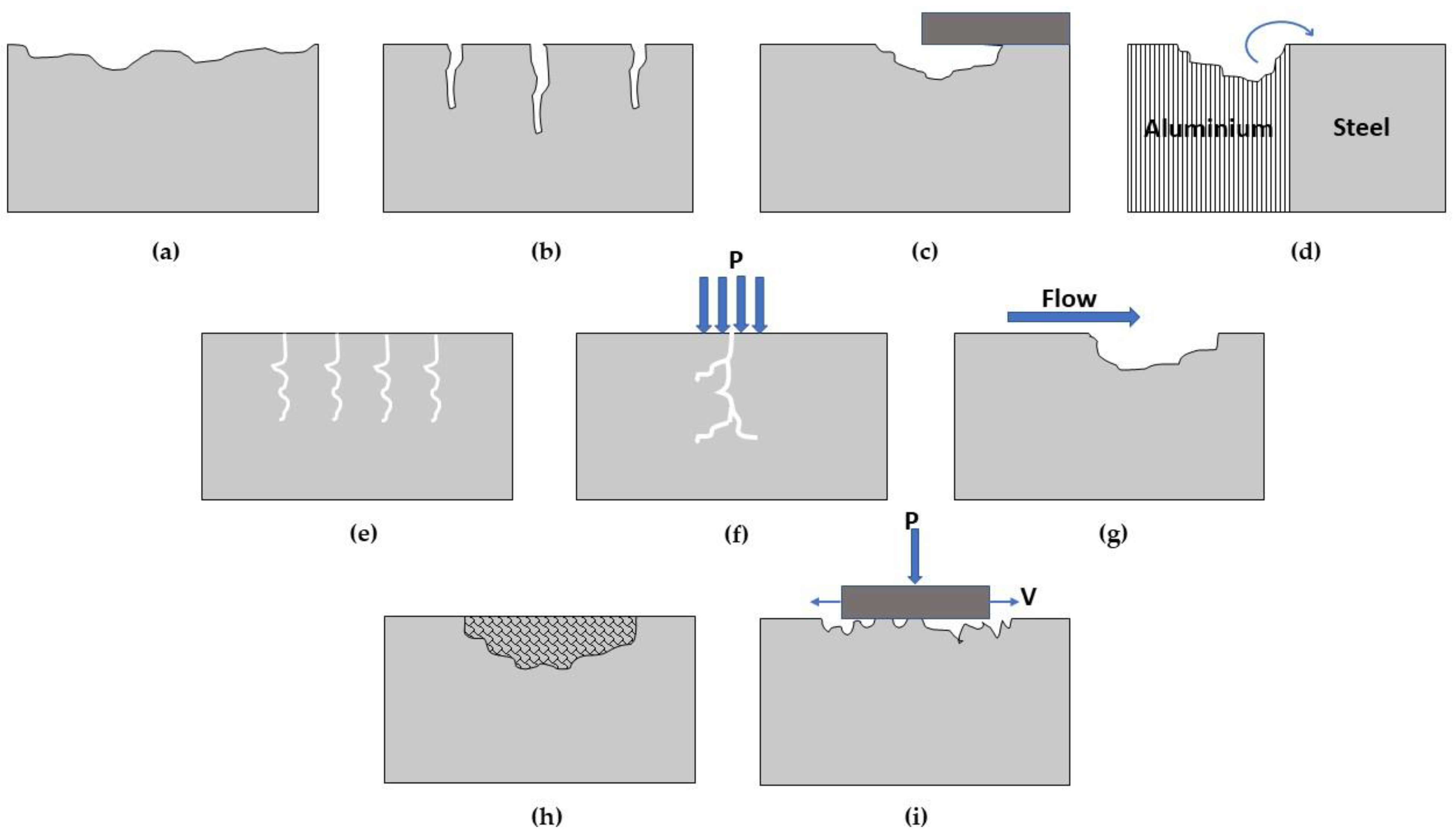
• Uniform corrosion: generating a uniform layer of rust (formation of oxide) over the surface of the metal exposed to atmosphere. In principle, uniform corrosion can reduce the rate of corrosion by limiting the contact surface between metal and the atmosphere. This is the most common type of corrosion in steel bridges.
• Galvanic corrosion: When two metals with different corrosive potential are placed together with the presence of a corrosive environment (electrolyte), the current flow and hence corrosion damage occur.
• Pitting Corrosion: One of the most common forms of corrosion with local attack which sometimes taking the form of deep holes (pits) into steel surface. This kind of corrosion in the presence of imperfection in steel components or dirt on its surface can engender cracks into the metal surface.
• Crevice Corrosion: This type of localized corrosion occurs by the differences between ion concentration in dissimilar environments (different ion concentration) inside and outside of the small crevice.
• Erosion Corrosion: When flowing of fluid with the relatively high velocity attacks over the surface of the metal, it can remove the coating film and accelerate the corrosion process.
• Stress Corrosion: In the presence of corrosive environment and applied tensile stress, brittle cracking occurs into the metal.
• Fatigue Corrosion: Repeated applied load with the corrosive environment causes stress concentration which leads to cracks into the metal.
• Fitting Corrosion: When two surfaces are in close contact in the presence of load provoke the abrasion of the surfaces by oxide.
• Intergranular Corrosion: The corrosion attack between steel grain boundaries which affect the mechanical properties of the material.

Figure 2. Prevalent forms of corrosion in steel structures: (a) uniform; (b) pitting; (c) crevice; (d) galvanic; (e) fatigue; (f) stress; (g) erosion; (h) intergranular; and (i) fitting corrosion.

Figure 2. Prevalent forms of corrosion in steel structures: (a) uniform; (b) pitting; (c) crevice; (d) galvanic; (e) fatigue; (f) stress; (g) erosion; (h) intergranular; and (i) fitting corrosion.

This research focuses on the outdoor atmospheric corrosion as the most common form of corrosion in steel structures.

There are several factors that affect the rate and progress of corrosion including environmental effects such as temperature, moisture, atmospheric pollutants (sulfur and chloride), type of material (different grade of steel), protection techniques and presence of crevice, stress or pollutants. The presence of these detrimental factors initiate corrosion and thus, decrease the capacity and make tremendous economic losses [14,15]. In the following section, a brief overview of the available models in the literature are discussed.

3. Corrosion Modeling

The existing numerical models are divided into two groups, namely heuristic and deterministic. Deterministic approaches are multi-scale models that account for the fundamentals of corrosion mechanisms to simulate the corrosion rate. Simulating the kinetics of a corroding system and/or metal-electrolyte interface to describe the corrosion rate can improve the robustness of the model. However, the model can become complex when several parameters are considered, referring to the interaction with gaseous and liquid environment, anodic and cathodic reaction of zinc and iron as well as diffusion of oxygen in immersed conditions [16]. On the other hand, the heuristic models that the present study focuses on are described from the regression of measured data, e.g., weight loss measurements or corrosion rate as a function of varied environmental parameters, e.g., temperature, relativity humidity, time of wetness as well as chloride deposition and time. Thus, they are simple in calibration, though they cannot be applicable to environmental conditions other than the one that the model was calibrated for. In general, it is possible to divide this approach into first and second level. The first-level studies the model from the initial chemical compound which initializes damage. The second-level, which the present study focuses on, interests engineers and is obtained from the observation and statistical analysis of experimental data with respect to the time of exposure.

The power function models (heuristic) were calibrated in different environmental conditions. The problem of these models pertained to the deficiency of a sufficient number of environmental factors in the calculation of the corrosion loss. To calculate the corrosion depth (in μm or g/m²) for the long-term, the time-dependent model that relates the corrosion loss at the first-year of exposure (A) with time according to the statistical analysis of the experimental data was obtained as follows [17]:

$$d\left(t\right)=A{t}^B$$

(2)

where A is the first-year corrosion rate, B is the coefficient which shows the long-term exposure effect considering the effect of protective products and environmental factors and t is time of exposure in years. From the mathematical point of view, if B > 1, it is clear that the corrosion process is accelerated. Alternatively, in the case of B < 1, the deceleration of process governs the corrosion loss and if B = 1, the corrosion rate is constant. Generally, when the coating layer is damaged, the corrosion process starts. This process ends when the rust layer covers all the steel surface.

As mentioned by Benarie and Lipfert [17], the B coefficient shows the chemical activity and performance of the product layer on the metal’s surface, which is influenced by the environmental factors and pollutants. Based on the collected data in this paper, the estimation of A (first-year corrosion rate) for steel was identified with concentration of sulfur ions (SO₂), and the calculation of the B coefficient was found based on the average rain pH. Few years later, Feliu et al. [18,19] proposed a similar power model (Equation (1)) accounting for the A value as the relation between different pollutants and metrological parameters in the form of binary interactions. Moreover, the value of B for different environmental conditions was discussed. Furthermore, Ma et al. [4] proposed A and B coefficients by accomplishing several experiments on mild carbon steel with different distances from the sea in a tropical marine environment over 3 years. They showed that due to the presence of chloride ions (Cl⁻) adjacent to the sea water (marine environment), the transition point (where the corrosion rate changes with respect to time) moved forward compared to the industrial atmosphere.

International Standard ISO 9224 in 1992 [20], provides a bi-linear model which states that the corrosion loss is in accordance with two separated linear parts (see Equation (3)). This general model divides the corrosion process into the initial average corrosion rate (r_av) and subsequent years based on the average steady corrosion rate (r_lin) up to the 10th year. It is assumed that the corrosion rate will be diminished after 10 years due to the creation of rust layers. These average corrosion losses are revised in the latest reports of ISO in 2012 [13,21].

$$d\left(t\right)=\{\begin{array}{cc}\hfill r_{av} t,& \hfill t<10\\ \hfill r_{av}·10+r_{lin} \left(t-10\right),& \hfill t\ge 10\end{array}$$

(3)

where t is time of exposure during the structure lifetime.

A similar power-linear function method is studied in 2016 which appropriate for up to 50 years old structures and the results are valid just for C1 to C3 corrosivity classes [22]. They concluded that after six years exposure of the structure in corrosive environment, the corrosion rate remained constant with respect to time (steady-state phase; r_lin, in Equation (3)).

Additionally, a new power-linear model was described by [21]. In this case, the corrosion rate becomes linear after 20 years of exposure (Equation (4)) and it is given by:

$$d\left(t\right)=\{\begin{array}{cc}\hfill r_{cor}{t}^B,& \hfill t\le 20\\ \hfill r_{cor} \left[{20}^B+B \left({20}^{B-1}\right) \left(t-20\right)\right],& \hfill t>20\end{array}$$

(4)

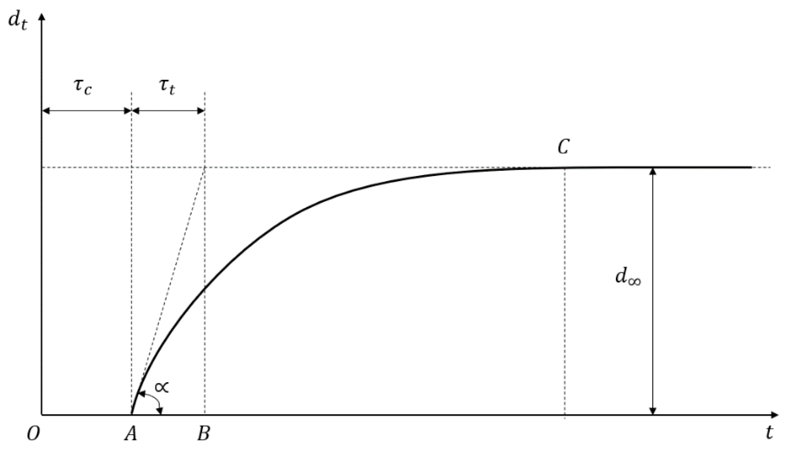
where $r_{cor}$ is the corrosion rate in the first year of exposure in grams per square meter per year (g/(m²·yr)) or micrometer per year (μm/year) consistent with ISO9223 [13]. Adjustment work reported by Albrecht and Hall Jr in 2003 [23] where the steady-state point was modified to subsequent years after the first year of exposure (instead of year 10 in Equation (3)). A nonlinear time-dependent model was recommended by Soares and Garbatov [24] in 1999, was separated into three main parts (Figure 3). At the first stage (OA) there is no corrosion due to the presence of protection layer. The second part (AB) is the initiation of corrosion because of damage to coating layer. The slope of the plot (corrosion rate) decreases until the corroded layer appears on the entire element surface (zero corrosion rate at C). This model can be utilized in different environmental conditions (Equation (5)) and it holds that:

$$d\left(t\right)=\{\begin{array}{cc}\hfill d_{\infty }\left(1-e^{-\left(t-{\tau }_c\right)/{\tau }_t}\right),& \hfill t>{\tau }_c\\ \hfill 0,& \hfill t\le {\tau }_c\end{array}$$

(5)

where ${\tau }_c$ is coating life, $d_{\infty }$ is the long-term thickness of the corroded component and ${\tau }_t$ is transition time which is calculated as $d_{\infty }/tg\propto$.

Indeed, corrosion initiates after damaging the protection layer (coating) and continues until the connection between metal surface and atmosphere stops, and the corrosion rate becomes zero. This model is calibrated with the data on member of bulk carrier in marine environment [25].

A model was represented in 2003 by [26], considering the interaction between corrosion protection system and environment as pitting corrosion, before the coating layer was completely damaged. In other words, after the coating layer loses its effectiveness, the general corrosion starts, and the corrosion rate decreases due to development of corrosion products on the metal surface. A few years later a new model considering the interaction between environmental variables (TOW, sulfur oxide, chloride and annual temperature) was proposed which represented in the form of dose-function model as follows [27]:

$$d\left(t\right)=A· t^{B }{\left(\frac{TOW}{C}\right)}^D· {\left(1+\frac{\left[S{O}_2\right]}{E}\right)}^F·{\left(1+\frac{\left[Cl\right]}{G}\right)}^H· e^{J\left(T+T_0\right)}$$

(6)

where TOW is annual time of wetness (h/year), T is air temperature (C) and A, B, D, E, F, G, H, J and T₀ are coefficients proposed in the paper.

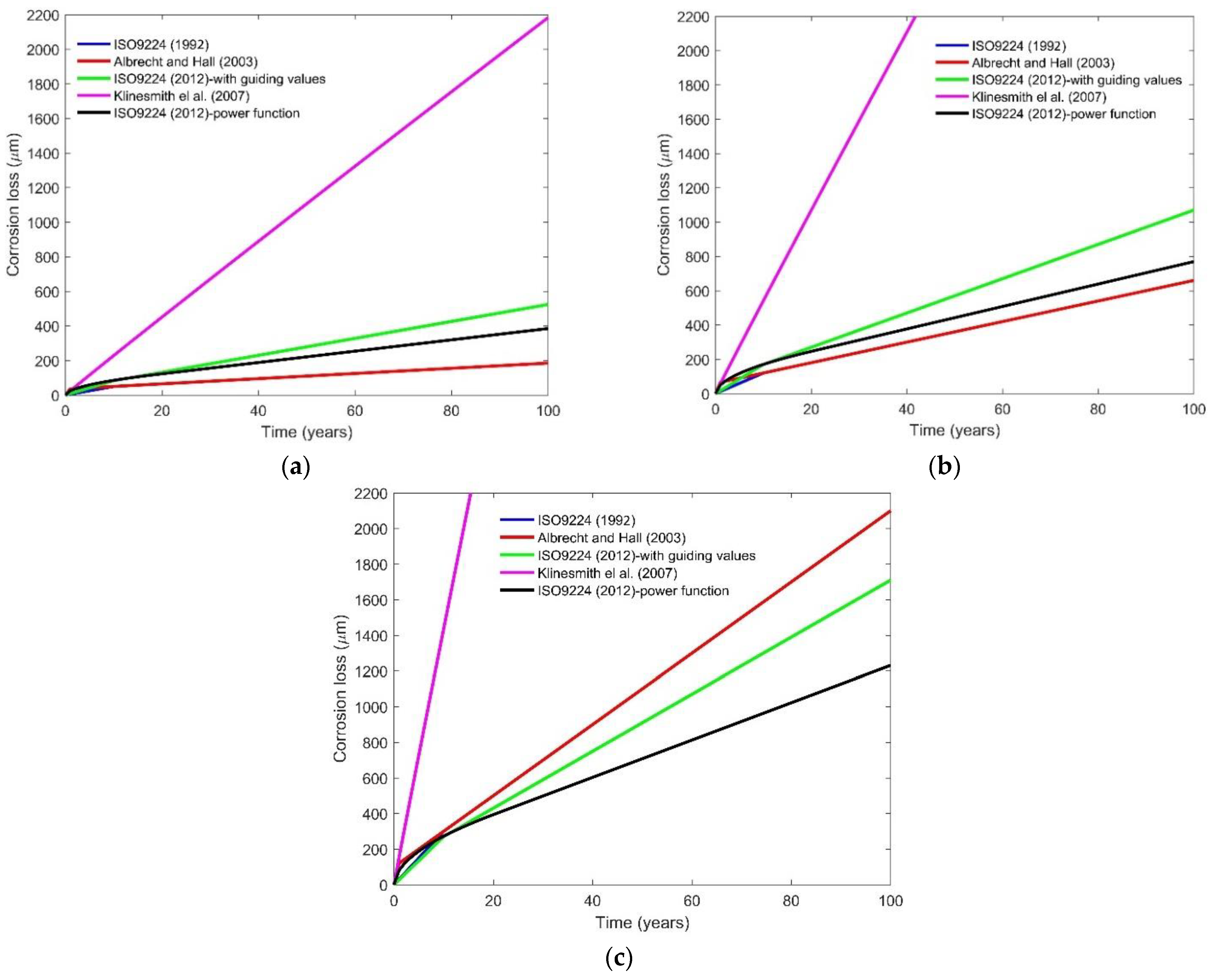
In Figure 4, the comparisons among selected models in atmospheric environment are displayed from low to high class of corrosivity using MATLAB programming software [28].

The corrosion loss before the 10th year are relatively close in all approaches, except in Klinesmith et al. model [27]. Results show that Klinesmith et al. [27] model overestimated the corrosion loss in long exposure of time, and accordingly, this model is not appropriate for estimating the corrosion loss in long-term. It should be noticed that the ISO9224 (1992) model [20] is similar to Albrecht and Hall Jr method [23] with different transition point.

4. Case Study Model

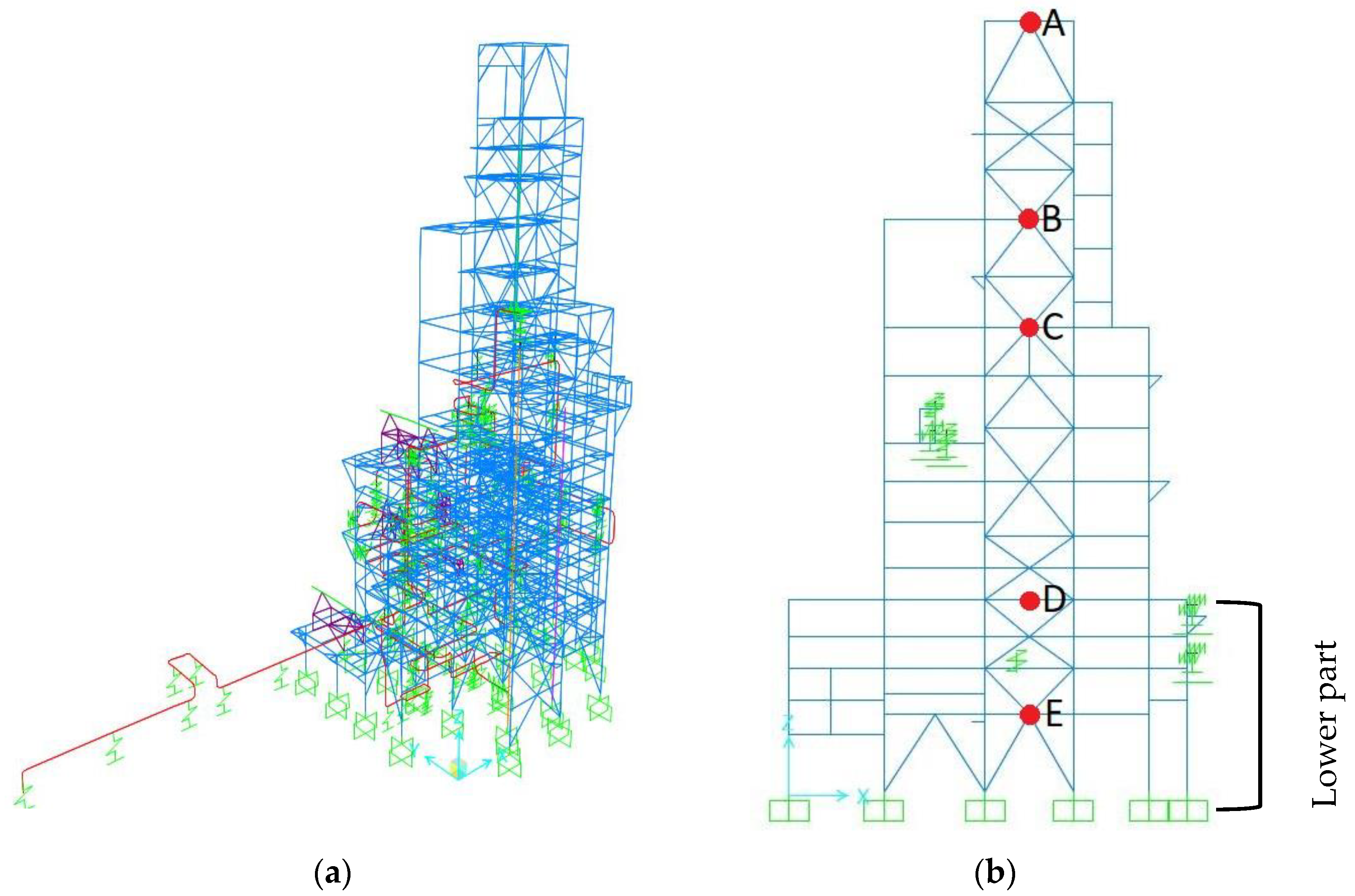
For evaluating the performance and identifying the dynamic response of structures, an irregular petrochemical steel tower is taken as a testbed so as to verify the effectiveness of corrosion damage to the structural behavior at different corrosivity levels.

The building is located in the Caribbean region with tropical environment, 61.30-m high, made of steel with 7682 kg/m³ density, 200 GPa module of elasticity and 250 MPa of yield strength. It comprises a steel braced frame and ordinary moment frame (OMF) as lateral resistance systems in X and Y directions, respectively. To examine the influence of flexibility of the beam-to-column connections, mainly in the X direction, two different lateral resisting systems were calibrated. In addition to the original system, a dual system was modelled with both directions being restricted. After comparing the vibration modes for the two different structural types, it was concluded that the maximum difference was 8% and 2% in the X direction and Y direction, respectively. Given that the flexibility of connection did not influence considerably the response, the original configuration of frames was considered in the assessment. Finally, the column nodes at the base are assumed to be fixed. column-base connections are assumed to be fixed. The design was performed following American design codes [29,30,31]. Figure 5a,b shows a 3D and a plan view of the process unit, respectively.

High percentage of mass is concentrated at the lower part of the building because of the significant number of equipment and vessels which have substantial role in the dynamic response of the steel tower. Point hinges are allocated at both ends of the beam and column elements to account for the plasticity of structural members.

Table 2. Seismic assessment parameters.

Parameter	Value
Occupancy/risk category	III
Seismic design category	D
Importance factor (Ie)	1.25
Short period acceleration (Ss)	1.37 g
Long period acceleration (S1)	0.375 g
Site class	D
Fundamental period (Ta)	1.30 s

summarizes several design parameters which are useful for the assessment in the following. In particular, the process unit is classified into risk category III [29]; given that the tower processes hazardous and toxic substances that can expose human and environment at risk. The long and short period acceleration, S₁ and S_S, for the site of interest are equal to 0.375 and 1.37 g, respectively, which classify the structure into seismic design category D. The seismic hazard of the site was derived from Bozzoni et al. [32]. Finally, the importance factor, site class and first vibration period were set equal to 1.25, D (V_s,30 = 187 m/s) and 1.30 s.

According to a local Environmental Management Authority (EMA) annual report [33], the average annual maximum temperature in the region of interest was 31.26 °C and the PM₁₀ concentration (particulate matter less than 10 microns in size) was estimated around 29.7 μg/m³. Additionally, based upon the recent report of this environmental organization [34], reported from another station during the first half of 2021, the concentration of SO₂ was less than 0.5 ppb (2.66 μg/m³) and the average concentration of NO₂ was estimated at 6.8 μg/m³ (Table 3). The annual average relative humidity (RH) was assessed around 82% in last year (over 80% for 9 months).

Table 3. Annual mean pollutants.

Pollutant	EMA [33,34]	ISO9223 [13]
NO2	6.8 (μg/m3)	Rural atmosphere
SO2	<1.33 (μg/m3)	Rural atmosphere
PM10 *	29.7 (μg/m3)	Urban atmosphere
RH	82%	Industrial atmosphere

* It is reported around 34 μg/m³ in average at EMA recent report in 2021.

Table 3. Annual mean pollutants.

Pollutant	EMA [33,34]	ISO9223 [13]
NO2	6.8 (μg/m3)	Rural atmosphere
SO2	<1.33 (μg/m3)	Rural atmosphere
PM10 *	29.7 (μg/m3)	Urban atmosphere
RH	82%	Industrial atmosphere

* It is reported around 34 μg/m³ in average at EMA recent report in 2021.

Figure 5. Steel process unit using SAP2000 [35]: (a) 3D view and (b) 2D view.

Figure 5. Steel process unit using SAP2000 [35]: (a) 3D view and (b) 2D view.

According to the afore-mentioned environmental and meteorology reports and due to the tropical and industrial zone of the case study location and particularly high rate of humidity, ISO9223 prescribes that this area should be classified in C4 zone (high corrosivity level, see also Table 1).

To perform seismic analysis, the computational platform SAP2000 [35] was employed. Μodal and time history analyses were carried out for different corrosivity levels with respect to different exposure of time (from 10 to 100 years) to estimate the dynamic response of structure during its lifetime.

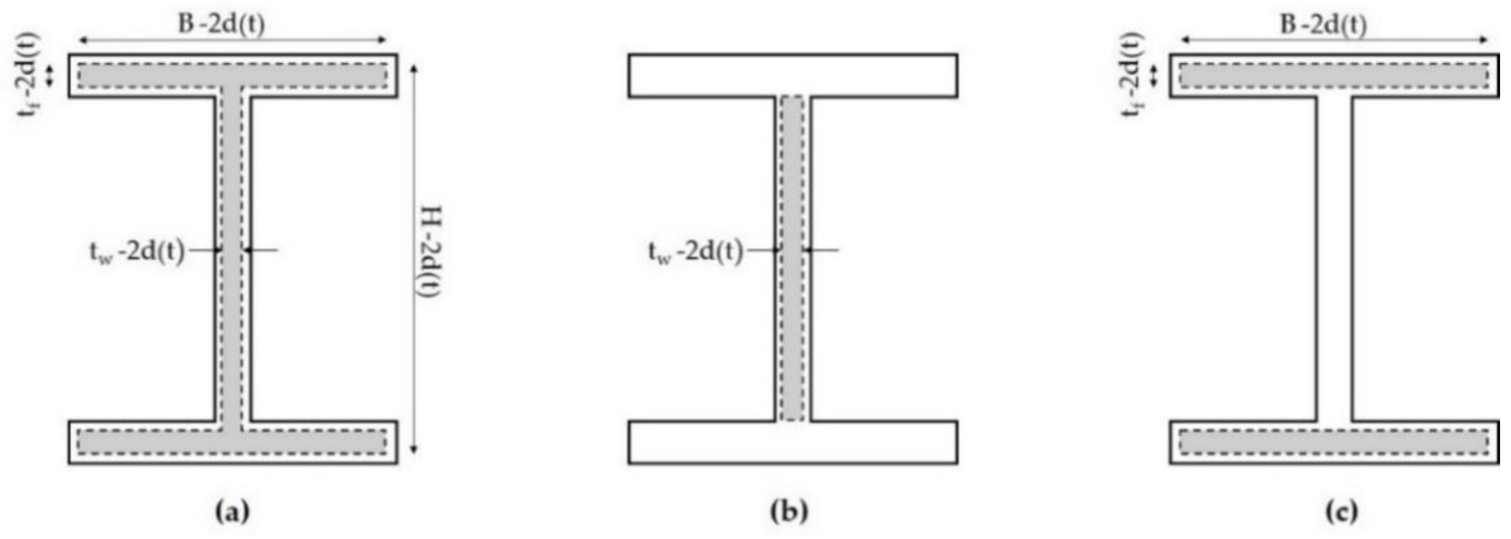
According to the available data from literature, the corrosion loss, d(t), was assumed as average uniform thickness reduction (in micrometer) [23]. In fact, the percentage of this reduction is not the same for the entire cross section; to this effect, different scenarios are studied, namely the mass loss of the entire cross section, the mass loss of the web only and mass loss of the flanges (Figure 6).

Wang et al. [6] proposed the following modified linear equations that account for the corrosion degradation through accelerated corrosion test:

$$\{\begin{array}{c}{f}_y=f_{y0}\ast \left(1-1.09\eta \right)\hfill \\ f_u=f_{u0} \ast \left(1-1.07\eta \right)\hfill \end{array}$$

(7)

where f_y and f_u are the yield and ultimate tensile strength of the corroded element, whereas f_y0 and f_u0 are yield and ultimate tensile strength of uncorroded part respectively and $\eta$ is the mass loss ratio. In this study, the computation of the mass reduction due to corrosion attacks from different outdoor atmospheric corrosivity levels (C2 to C4) is determined by different methods based on their highest influence. As demonstrated in Figure 4, the ISO9224 (2012) [21] model (with guiding values) for C2 and C3, and Albrecht and Hall Jr (2003) method [23] for C4 level have the highest effect between other approaches. Because of the overestimation of corrosion loss by Klinesmith et al. [27] in long term exposure and due to the similarity of ISO9224 (1992) method [20] with Albrecht and Hall Jr model [23], these models are not considered in the case study model.

To assess the response along the height of the structure, five nodes were taken in different levels, as shown in Figure 5b(A–E). The drifts and accelerations of these nodes were studied at each level of corrosivity. The square root of the sum of the squares (SRSS) rule was used to combine the results of both directions.

5. Seismic Response Analysis

5.1. Modal Analysis

To compute the dynamic response of the damaged (corroded) structure in linear region, the modal analysis was carried out during the structure life-time period. Due to the irregularity of the structure and in contrast with common buildings, the effect of higher modes is significant, whilst the first mode pertained to the equipment and vessels. In this study, the modes with mass participation higher than 10% were considered at each transitional direction (X and Y). Thus, mode number 4 and 11 in X direction and mode number 3 and 12 in Y direction were selected for comparing the period of vibrations at each corrosivity category (Figure 7). To account for corrosion effects, the thickness reduction approaches were adopted (Figure 6) and the results were compared and summarized below (Figure 8, Figure 9 and Figure 10). For consistency, the vibration period of corroded structure (T_C) was evaluated with respect to uncorroded model (T_UC).

5.2. Time History Analysis

In this study, a number of 20 far-field earthquake records are selected based on the conditional spectrum approach [36] provided by PEER strong ground motion database which are presented in

Table 4. Earthquake event and parameters of recorded ground motion for far-field records set.

Record No.	Earthquake Name	Year	Time Steps (s)	PGAY (g)	PGAX (g)
1	“N. Palm Springs”	1986	0.005	0.060	0.114
2	“Whittier Narrows-01”	1987	0.005	0.203	0.295
3	“Loma Prieta”	1989	0.005	0.072	0.074
4	“Loma Prieta”	1989	0.005	0.127	0.126
5	“Loma Prieta”	1989	0.005	0.192	0.140
6	“Loma Prieta”	1989	0.005	0.179	0.369
7	“Loma Prieta”	1989	0.005	0.215	0.204
8	“Landers”	1992	0.005	0.134	0.136
9	“Northridge-01”	1994	0.010	0.102	0.063
10	“Northridge-01”	1994	0.010	0.126	0.156
11	“Northridge-01”	1994	0.020	0.239	0.167
12	“Kocaeli_ Turkey”	1999	0.005	0.186	0.252
13	“Chi-Chi_ Taiwan”	1999	0.004	0.063	0.052
14	“Chi-Chi_ Taiwan”	1999	0.005	0.060	0.068
15	“Chi-Chi_ Taiwan”	1999	0.005	0.169	0.124
16	“Chi-Chi_ Taiwan”	1999	0.005	0.039	0.044
17	“Chi-Chi_ Taiwan”	1999	0.005	0.072	0.076
18	“Chi-Chi_ Taiwan”	1999	0.004	0.169	0.124
19	“Chi-Chi_ Taiwan”	1999	0.004	0.093	0.091
20	“Chi-Chi_ Taiwan”	1999	0.004	0.072	0.058

.

Nonlinear time history analyses were performed by taking the three thickness loss approaches into account (Figure 6). Additionally, the impact of corrosion on the mechanical properties of the structure was considered based on Equation (7), without reducing the geometric properties of the main model. In this method, the yield and ultimate tensile strength of the material were modified according to the mass loss at each class of corrosivity. For calculating the mass ratio ($\eta$), the thickness mass reduction method of the entire section in C4 level of corrosivity (proposed by ISO9223 [13]) was employed.

6. Discussion and Results

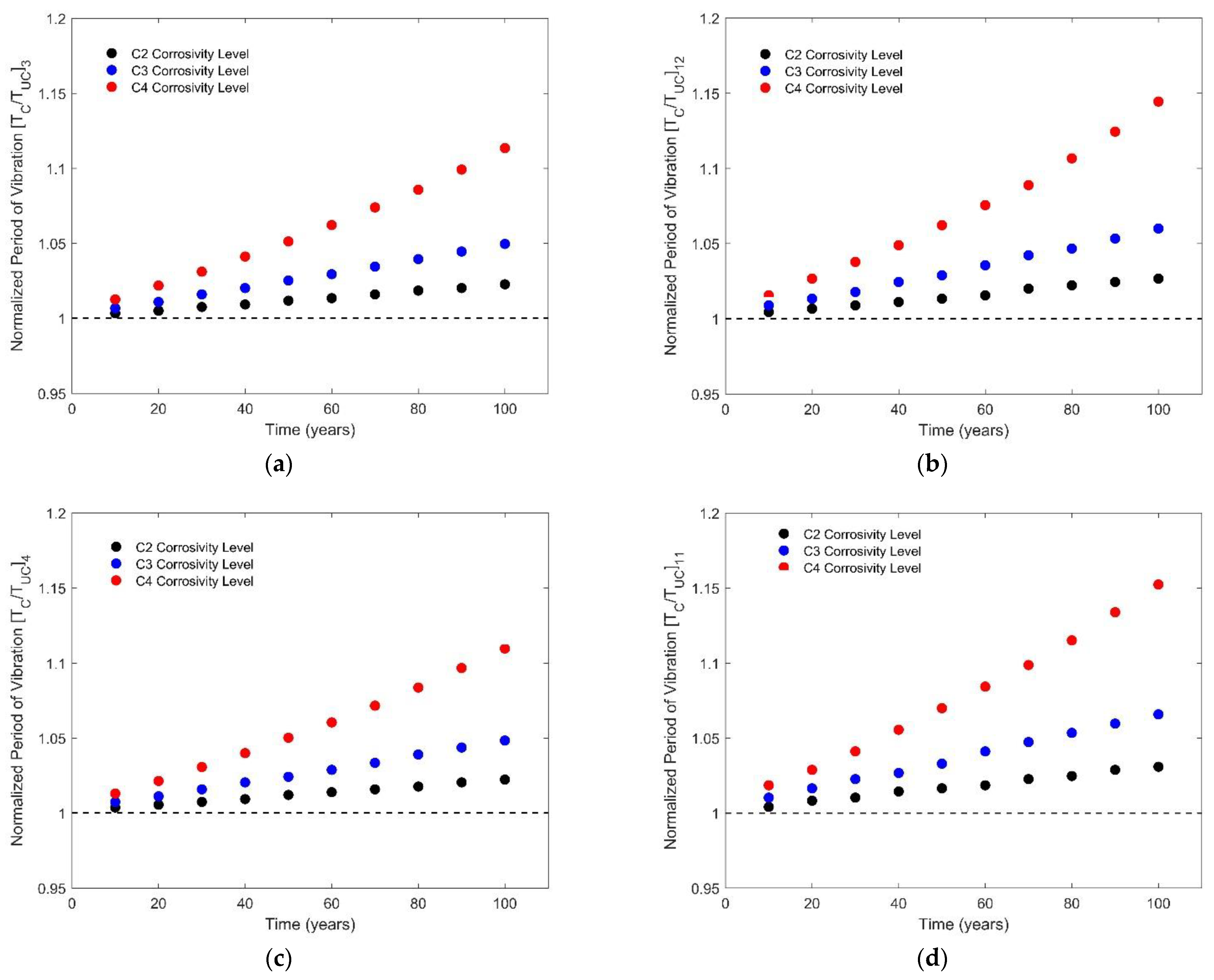
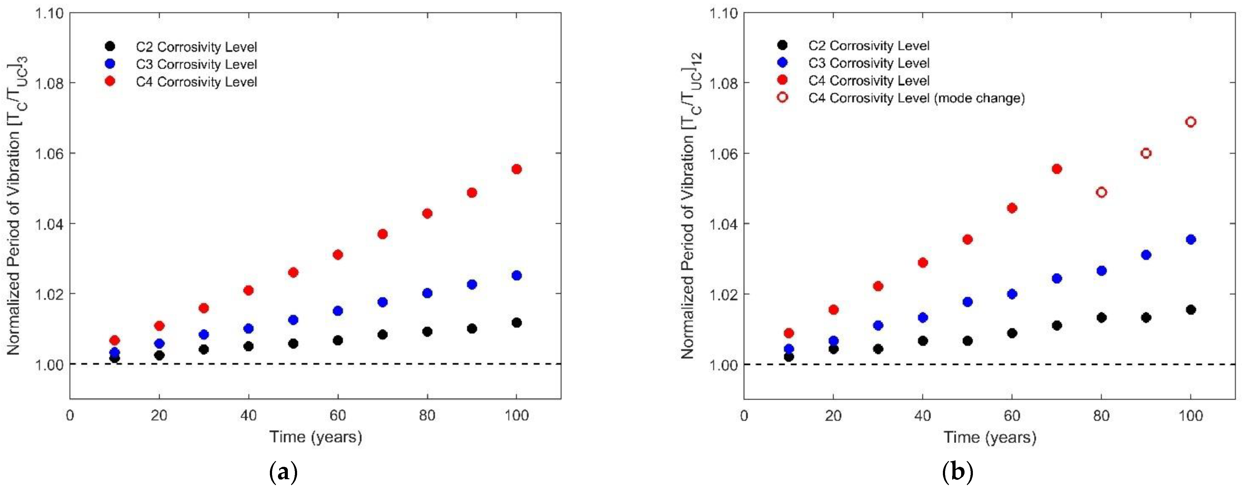
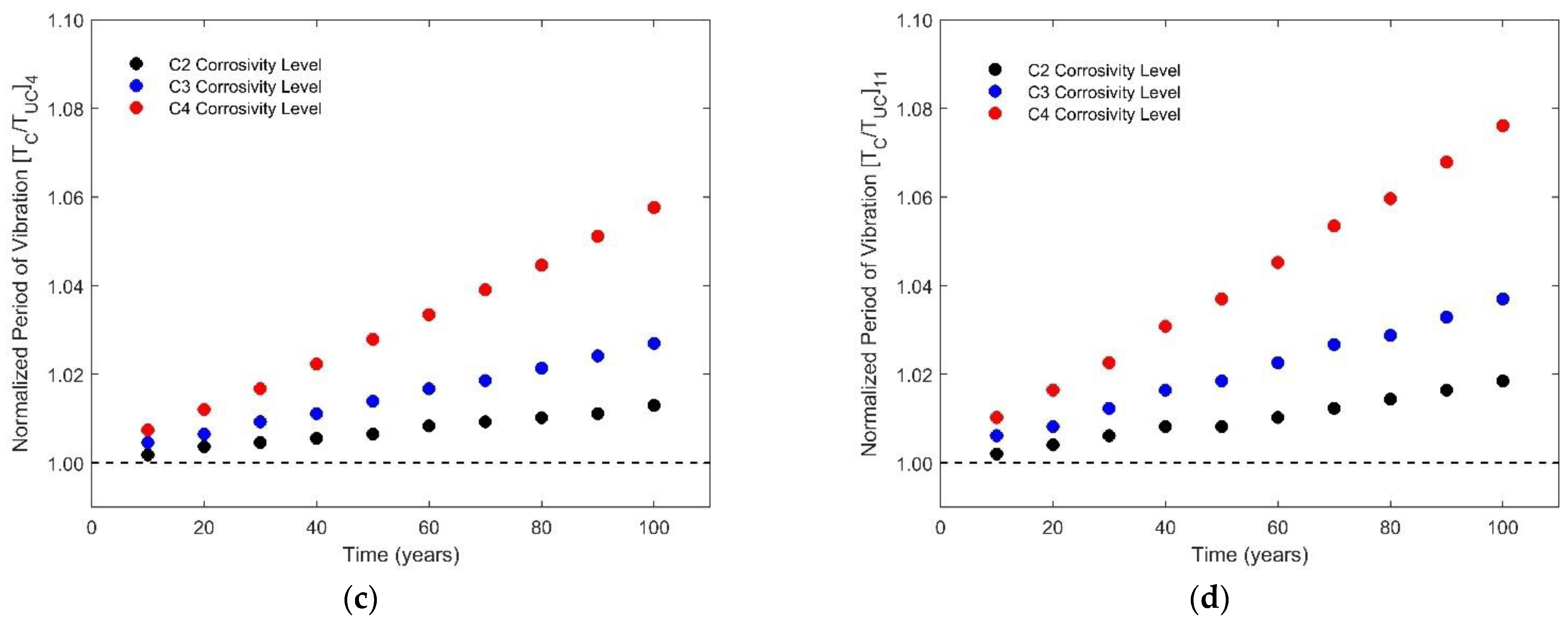
To compare the structural responses subjected to different corrosion classes in the linear region, modal analysis was employed, and the outputs are plotted for each mode separately. In the present paper, the effect of C2 to C4 corrosivity categories were considered, which referred to low (C2), medium (C3) and high (C4) levels of damage due to corrosion attacks.

The highest increase in the vibration period was observed in the case of corrosion on the entire section, corrosivity level C4 and 100 years lifetime, and it was equal to 15% approximately (see modes 12 and 11 in Figure 8b,d). In the rest of cases (Figure 9 and Figure 10), the corresponding rise was smaller than 8%. It is assumed that the reference period of the process unit under consideration is roughly 63 years (more details about the reference period for petrochemical plants can be found in [37]); hence, the vibration rises by 3%, 5% and 10% in the case of corrosion effect on web, flange and the entire section, respectively, regarding the C4 corrosivity level. Additionally, it should be highlighted that the structure experiences a sudden decrease in period of vibration after 80 years in C4 corrosivity level. This is because of the flanges mass loss that caused change in mass participation of modes (the change is illustrated by hollow circles in Figure 9b). It is concluded that the depth mass loss increases linearly with respect to period of time, as it was also illustrated in a recent study [2].

For assessing the performance and dynamic characteristics of corroded structure in nonlinear region, the time history analysis was employed. The time history analysis was considered as a powerful tool to accurately assess the seismic performance of the structure in different environmental conditions under dynamic loads. A comparison among all methods was performed at 20, 50 and 100 years of the building which refer to normal, design and long-term life of the structure, respectively.

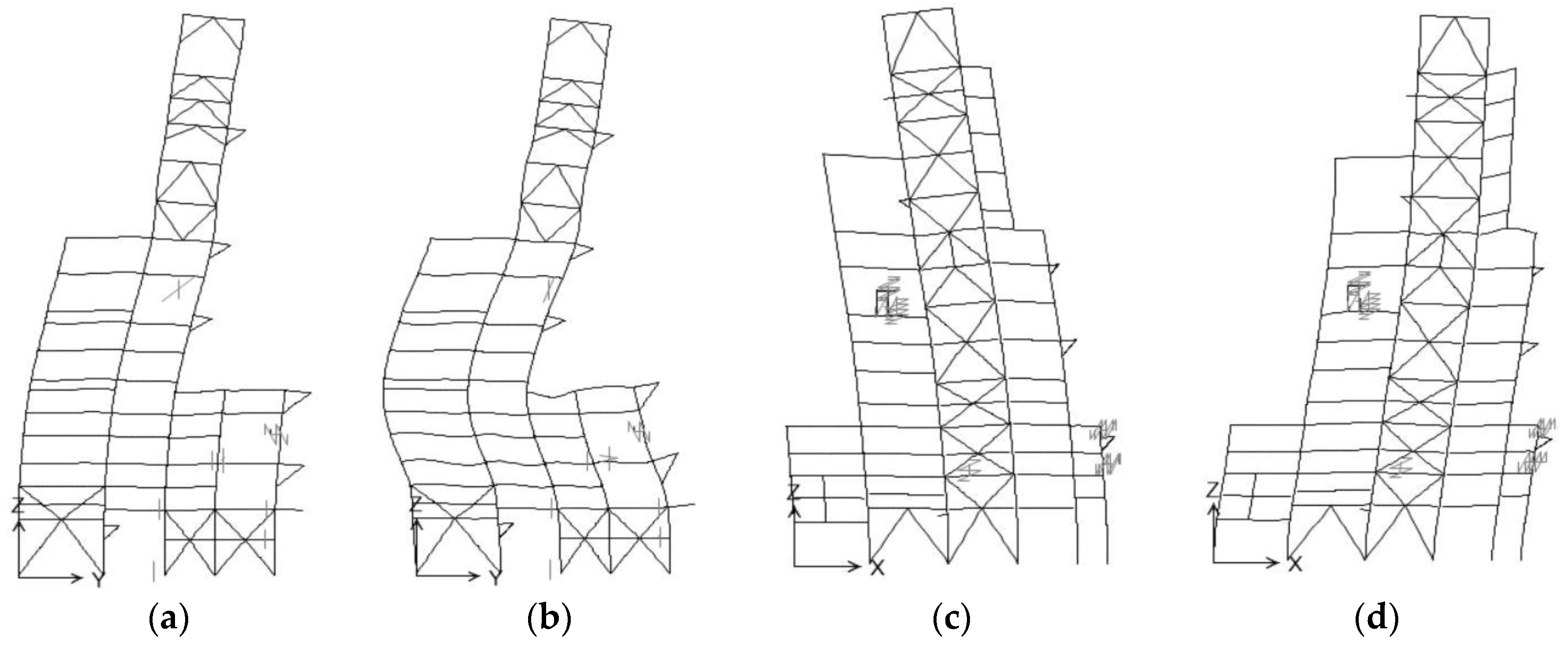
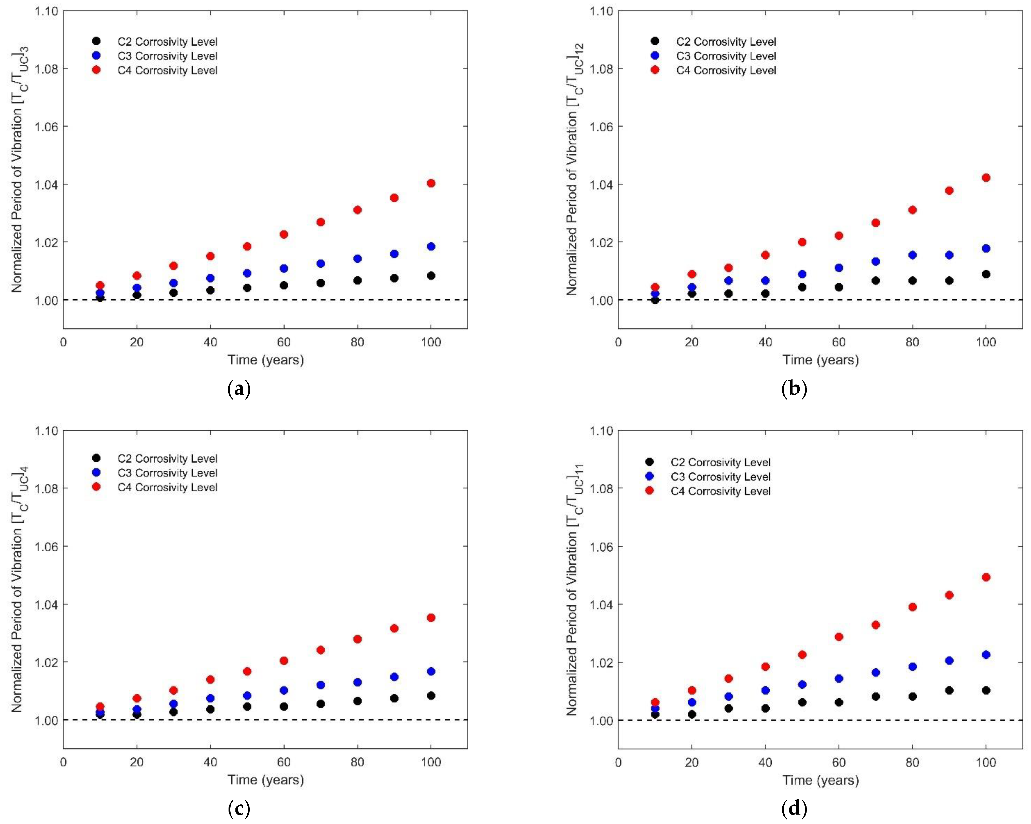
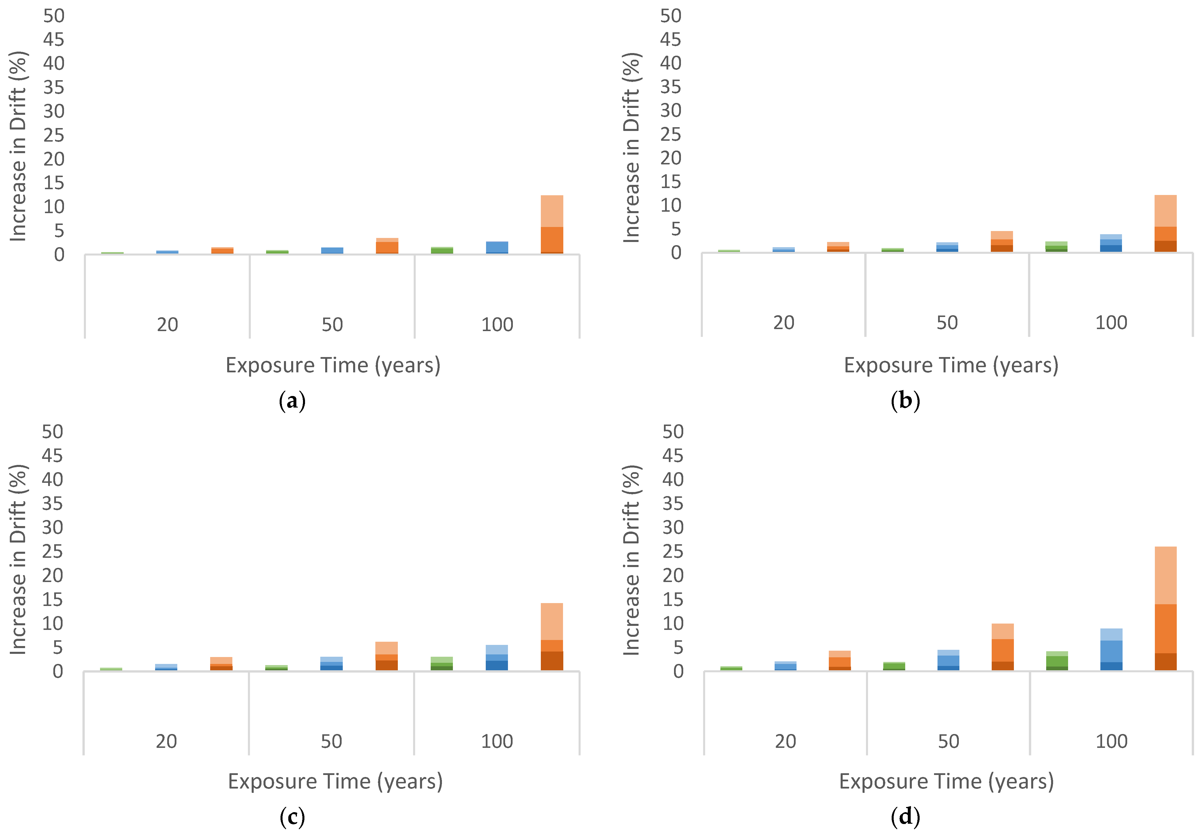
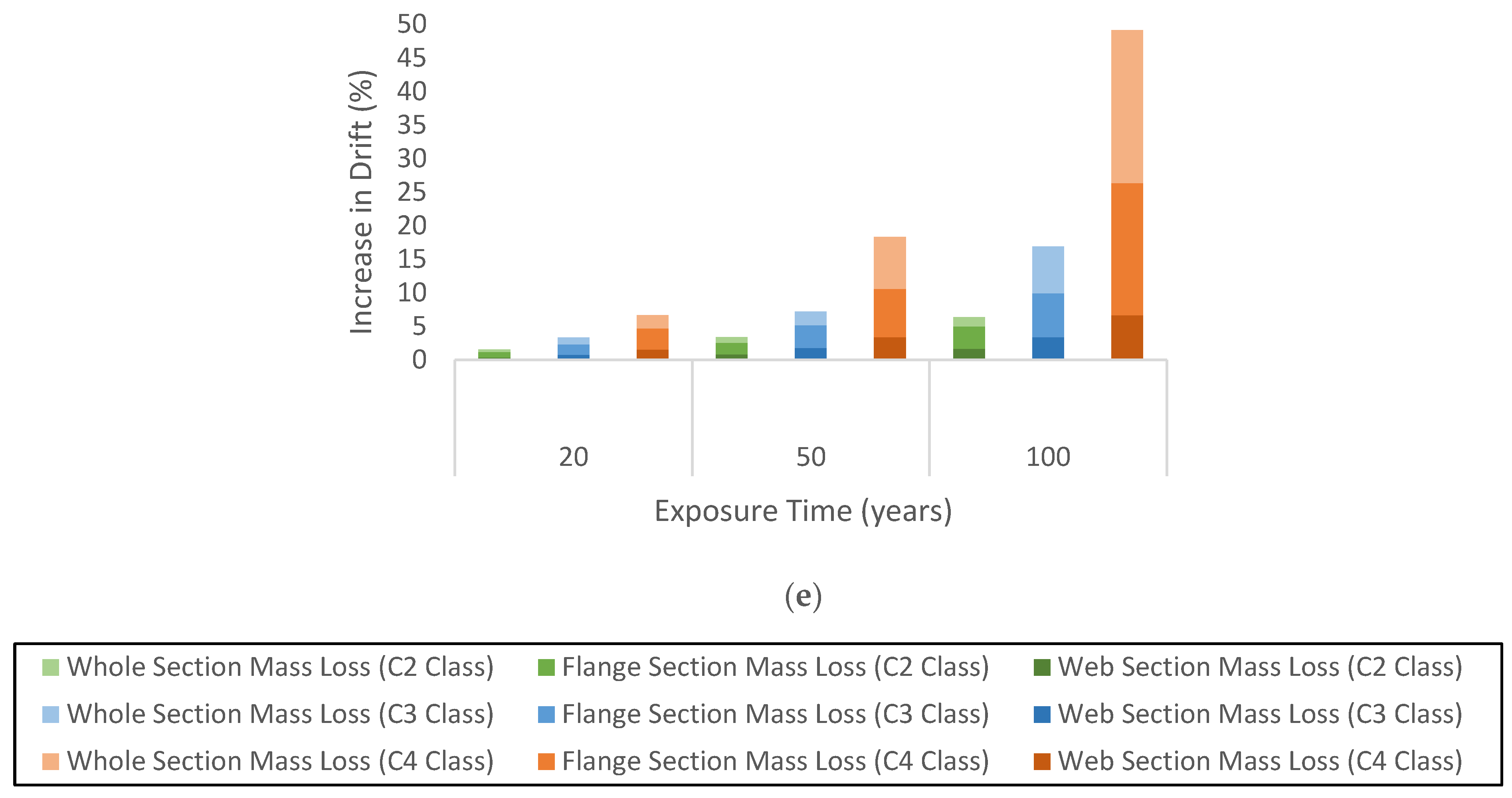
The combined lateral drifts in both X and Y directions of each node with respect to its height are evaluated and their differences are shown (see Figure 11). For consistency, the results are normalized to the uncorroded case value. As illustrated in Figure 11, node E experiences the highest impact compared with other nodes. This increase is approximately duplicated in the highest level of corrosivity in long-term life of the structure (damage of entire section in C4 level).

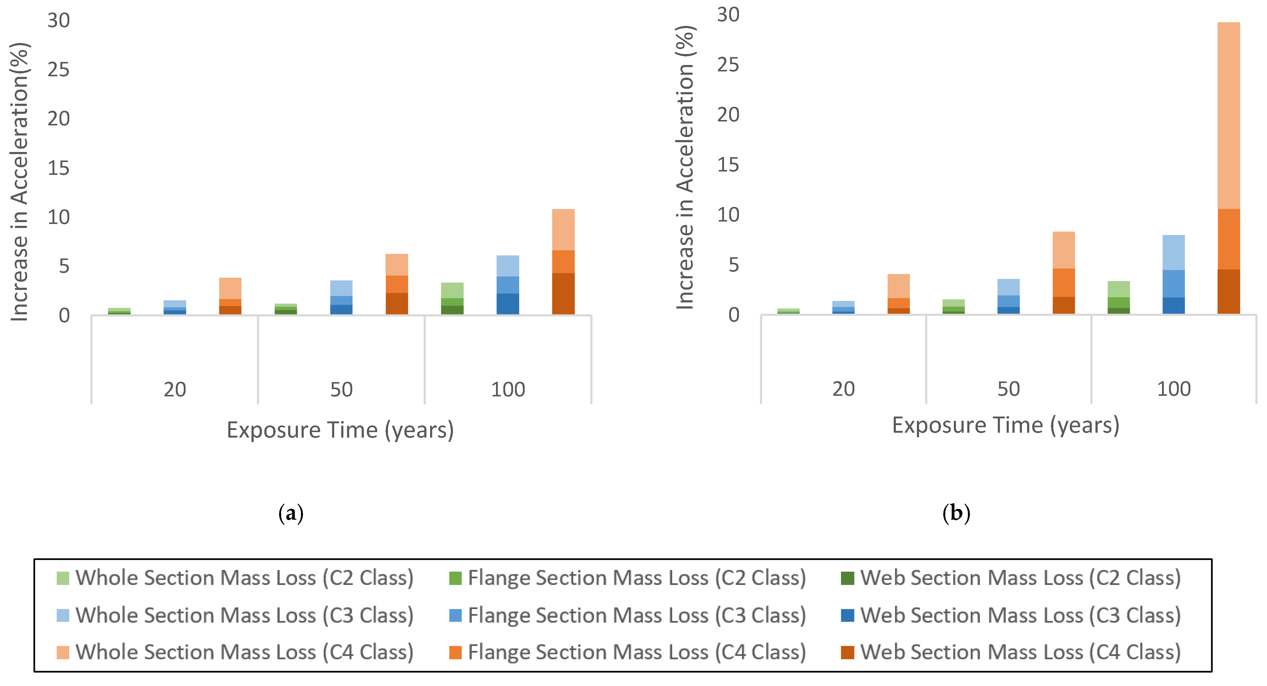
Similarly, the average combined peak acceleration of each node was evaluated, and the results are compared with each other in Figure 12. In particular, under the worst corrosion scenario model (entire section mass loss in C4 class of corrosivity), there is an increase by 29% in 100 years for node E. This value is 2.7 and 6.4 times larger in the same condition than using flange and web section thickness loss methods, respectively. The difference between the values of the acceleration in upper nodes (A–C) of corroded structure and acceleration of the uncorroded case was less than 10%.

It should be noticed that the change in the mechanical properties results in negligible impact on the drifts and accelerations (below 5%).

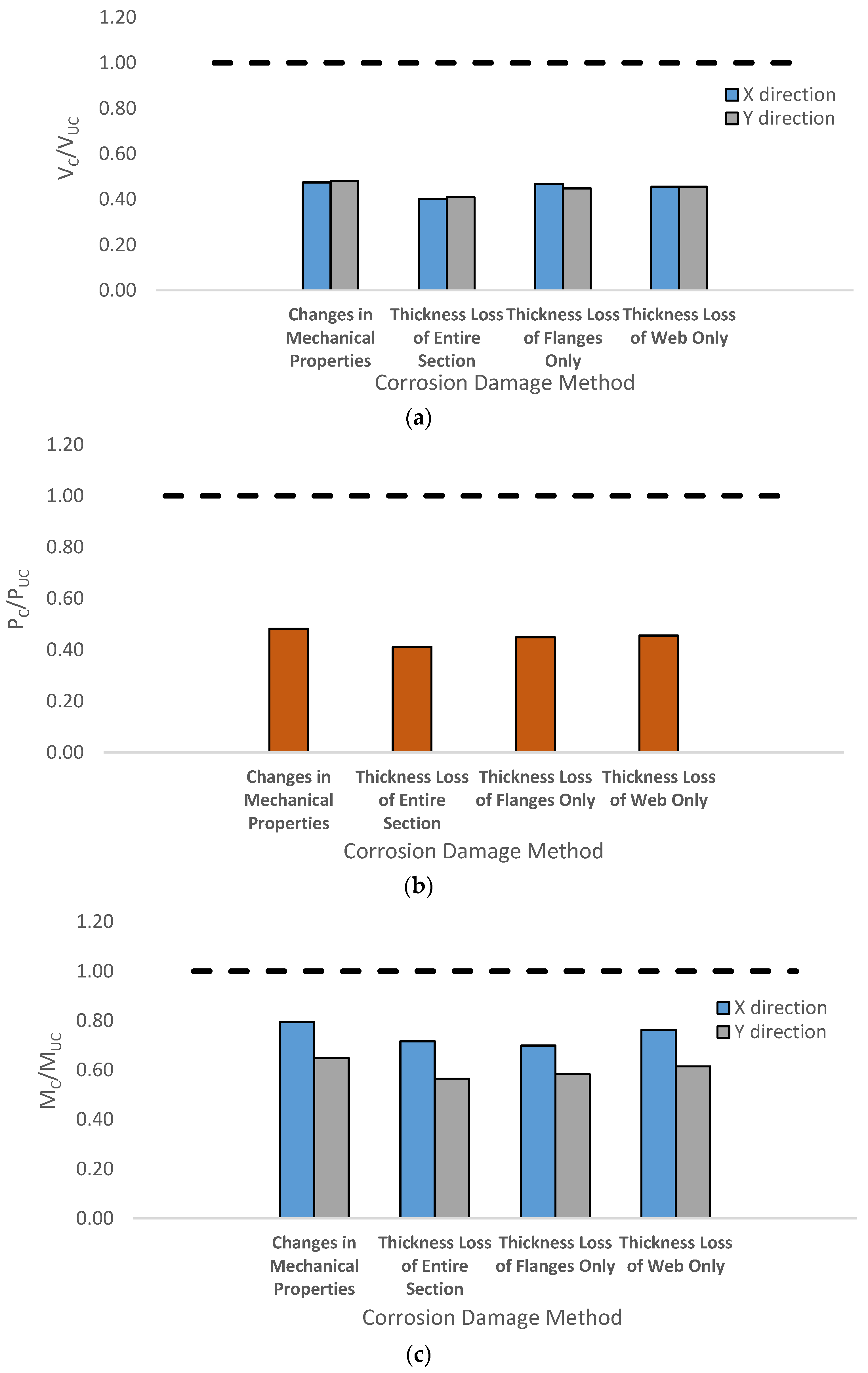
Severe corrosion damage affects the resistance capacity of the structure. This damage which is related to the changes of material properties or section thickness reduction results in changes in internal forces. To this effect, the worst scenario (widespread damage in C4 level of corrosivity at 100 years) of building was considered for all approaches to compare the response of the structure using different mass loss techniques. The resultant reactions from seismic loading with respect to the life time of the structure are evaluated for different forces. Figure 13 illustrates the variation of reaction forces of the building for all approaches in the worst environmental condition and long-term of exposure for each direction where V_C, P_C and M_C are the shear, axial and moment forces of corroded model, respectively, and V_UC, P_UC, and M_UC are for uncorroded model in the same order.

Figure 13 shows the reaction forces evaluated by different corrosion loss approaches in C4 level of corrosivity over a 100-year time period. To account for the mass loss ratio ($\eta )$ of equation 7, the entire section mass loss method was employed. The mass loss was roughly 29% with respect to uncorroded structure for C4 class which was the highest rate of damage in the case study model. Figure 13a represents the modification values of base shear evaluated through four methods that can be found in the literature. The results show that the base shear of the structure decreased by applying different corrosion damage scenarios. This reduction is around 60% for the entire section mass loss and it is nearly halved for other damage techniques. Furthermore, the reduction in the case of axial reaction was 60% lower compared to the uncorroded case, as shown in Figure 13b. The modification of moment reaction forces is shown in Figure 13c. The considerable reduction of moment force is observed for all the approaches. The decrease varies between 20% and 50%.

7. Conclusions

The effectiveness of different available thickness reduction corrosion models of structural steel has been discussed. Recently, new methods were proposed considering the effect of corrosion damage on the mechanical properties of the structure. However, there is a clear deficiency of probabilistic models that account for the corrosion rate in low to high rate of corrosion (C2 to C4 class). Indeed, most of the models were calibrated in a specific environment, which is mainly marine, and are useless in other environmental conditions, e.g., at urban zones.

The performance of a petrochemical nonbuilding structure was used as a testbed considering harsh environmental conditions based on real observations of the site that structure is located in. Firstly, the structure was analyzed in the linear regime, and it was deduced that the period of vibration increases linearly for each class of corrosivity during the life time of the structure with respect to the mass loss rate. Similarly, there was an increase up to 11% and 26% in structural drift and acceleration demand for the web section mass loss in long exposure of time. The increase in structural response in case of flange and entire section loss were smaller and higher, respectively, than the aforementioned values. For the structure with the C4 level of damage in 100 years, the increase of drift was 3× and 7.7× more than the drift for the C3 and C2 classes of corrosivity, respectively. The acceleration rise was 4× and 8× greater than for C3 and C2 damage levels, respectively. Negligible changes were observed by modifying the mechanical properties of the model (as a corrosion mass loss technique).

Finally, the bearing capacity of the main model has been compared with the corroded structure in the presence of highest rate of corrosion, using time history analysis and accounting for nonlinear material. The mass loss reduction resulted in the decrease of reaction forces of the corroded structure, which was nearly equal amongst the different corrosion damage methods. In particular, this reduction was at least 50% for axial and shear forces, whereas it did not exceed 45% for all corrosion damage methods.