
Diffuseness Quantification in a Reverberation Chamber and Its Variation with Fine-Resolution Measurements


Abstract
1. Introduction

| Category | Metrics | Reference | Measurement | Description |
|---|---|---|---|---|
| Homogeneity | The relative standard deviation of decay rate | ASTM C423-17 [1] | Decay rates or SPLs in multiple locations using fixed microphones or moving microphones. | Lower values of deviations across the sound field indicate higher diffuseness. |
| Total Confidence Interval | ASTM E90-09 [19] | |||
| The spatial standard deviation of the reverberation time | Bartel & Magrab [11], Davy [29] | |||
| Spatial Uniformity | Wang et al. [13] | |||
| Isotropy | The diffuseness estimate | Lokki [25] | Using spherical microphone arrays to analyze the direction of energy flow. | The isotropic sound energy from all directions means high diffuseness. |
| Directional Diffusivity | Gover et al. [26] | |||
| The spherical harmonic covariance matrix | Epain & Jin [27] | |||
| Wavenumber spectrum | Nolan et al. [16] | |||
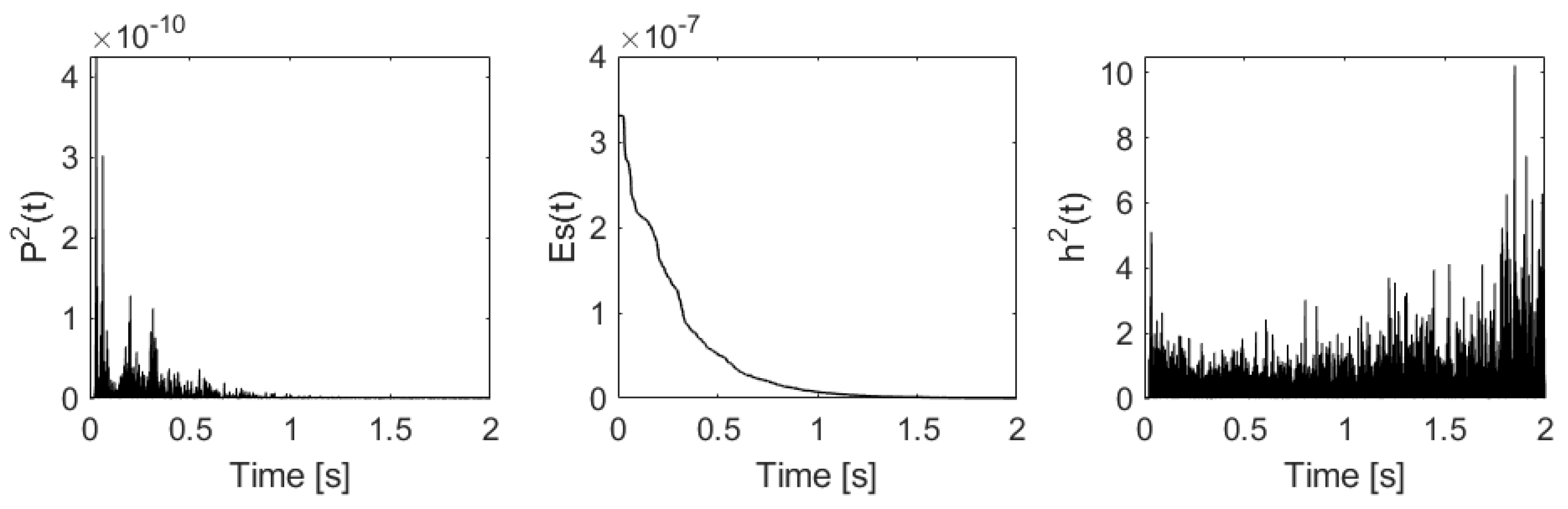
| Indirect method | Number of peaks | Jeon et al. [23] | Analyzing the details of the impulse response. | Less fluctuation of impulse response in the early decay means higher diffuseness. |
| Kurtosis | Jeong [15] | |||
| Mixing time | Prislan [26] | |||
| Degree of time fluctuation | Hanyu et al. [14,21] | |||
| Maximum absorption coefficient | ISO 354:2003 [2] | Measuring the sound absorption coefficient with an increasing number of diffuser panels. | The optimum diffuse configuration is achieved when it produces the maximum absorption. | |
| Reference absorber | Scrosati et al. [6] | Comparing the equivalent absorption area of the reference absorber with a minimum value. | The absorption correction factor can be used to quantify the reverberation chamber. |
2. Methods
2.1. Diffuseness Metrics
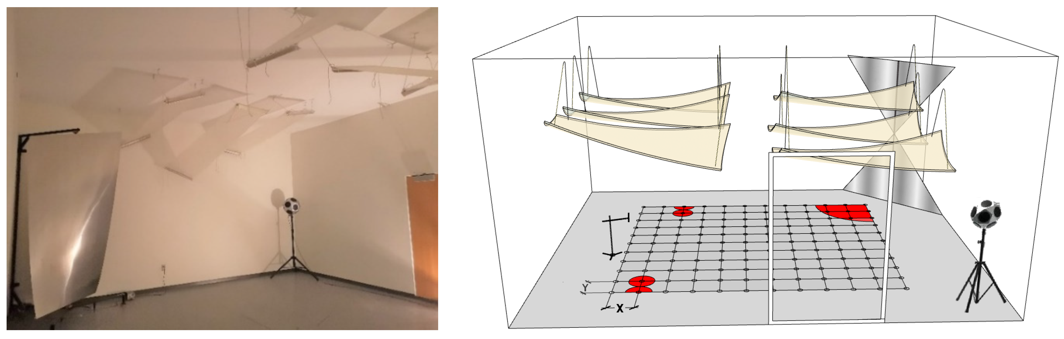
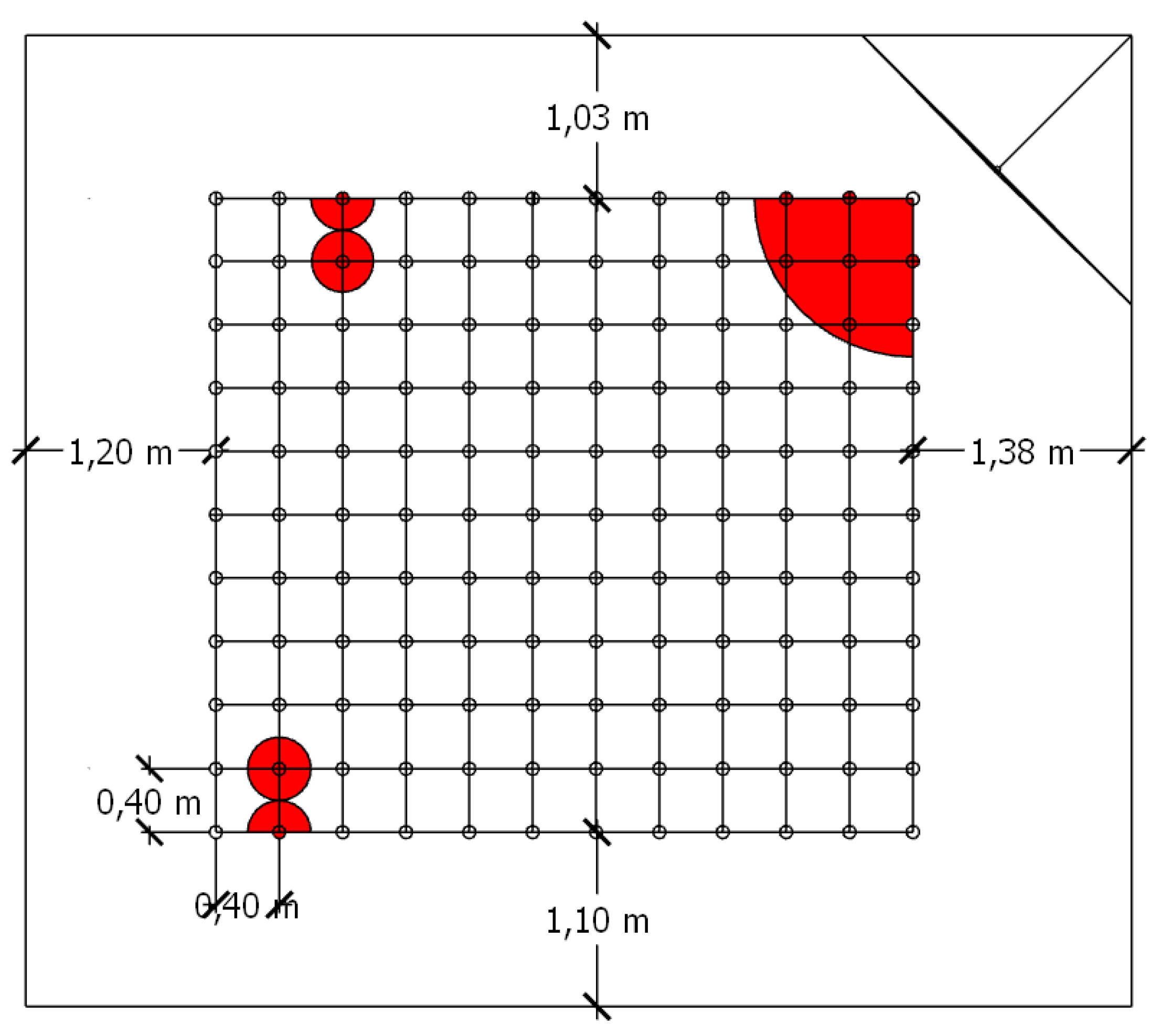
2.2. Measurement
2.3. The Number of Measurement Samples Required for Diffuseness Quantification
3. Results and Discussion
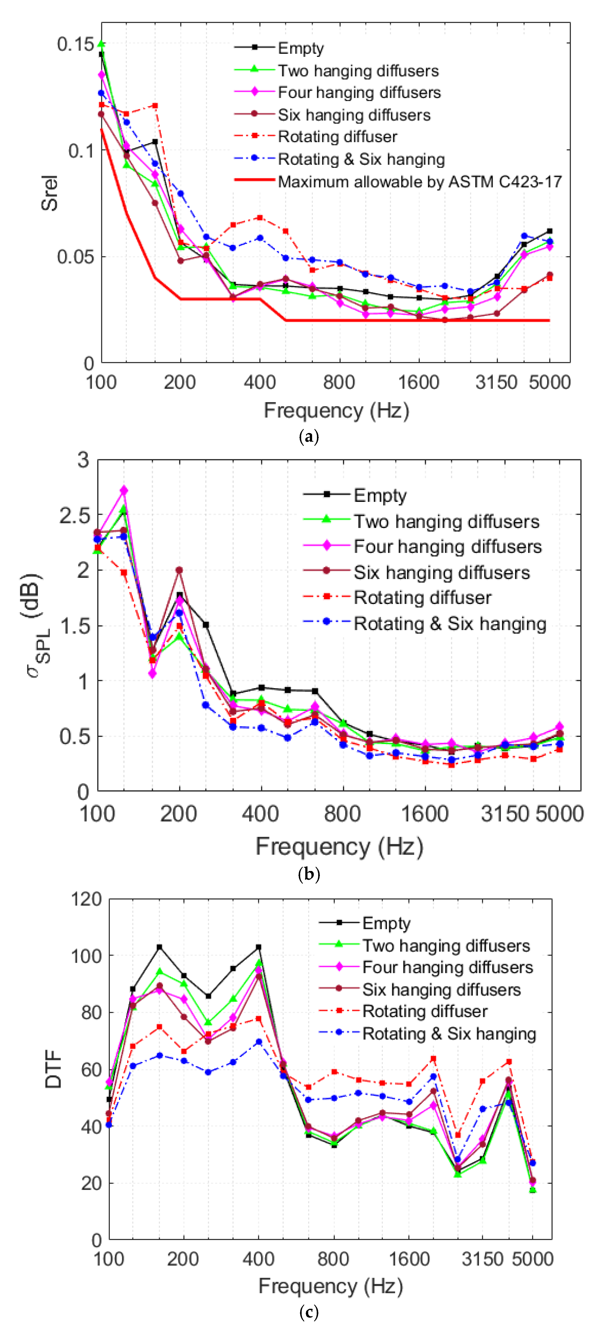
3.1. Diffuseness Quantification
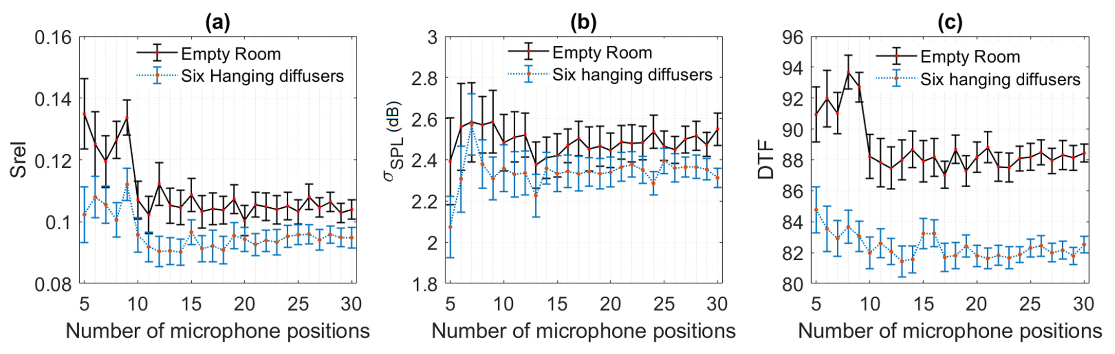
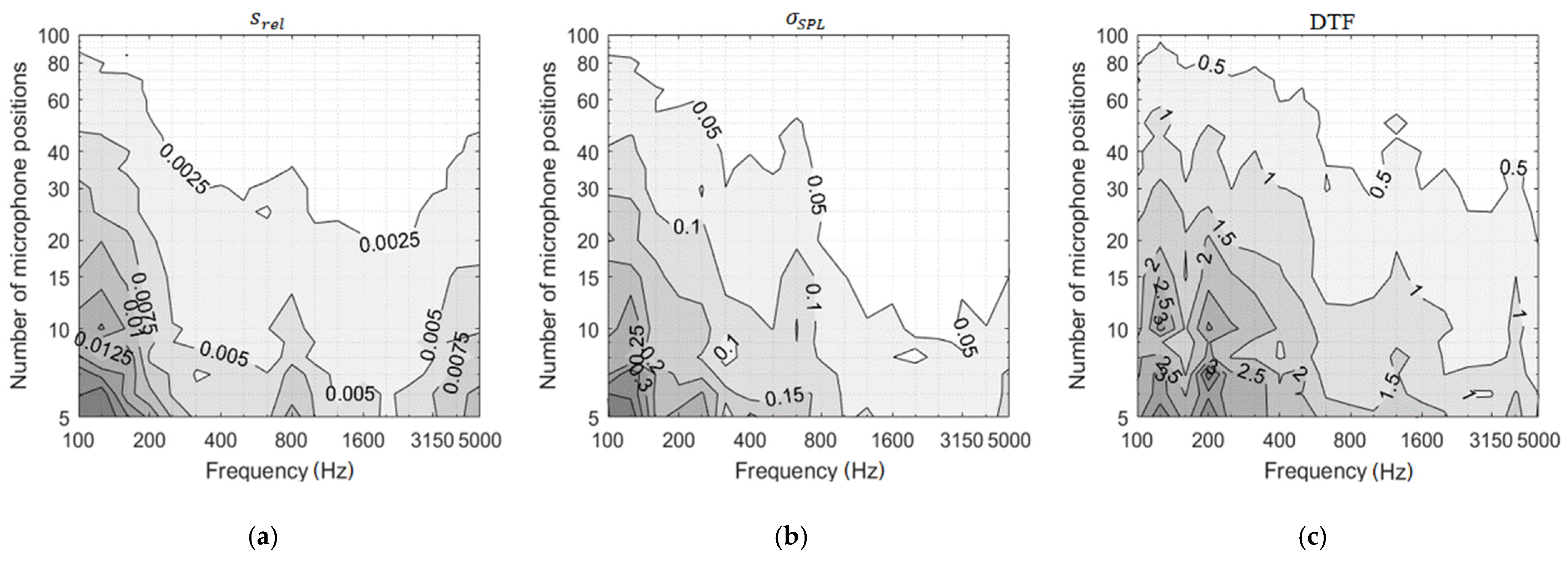
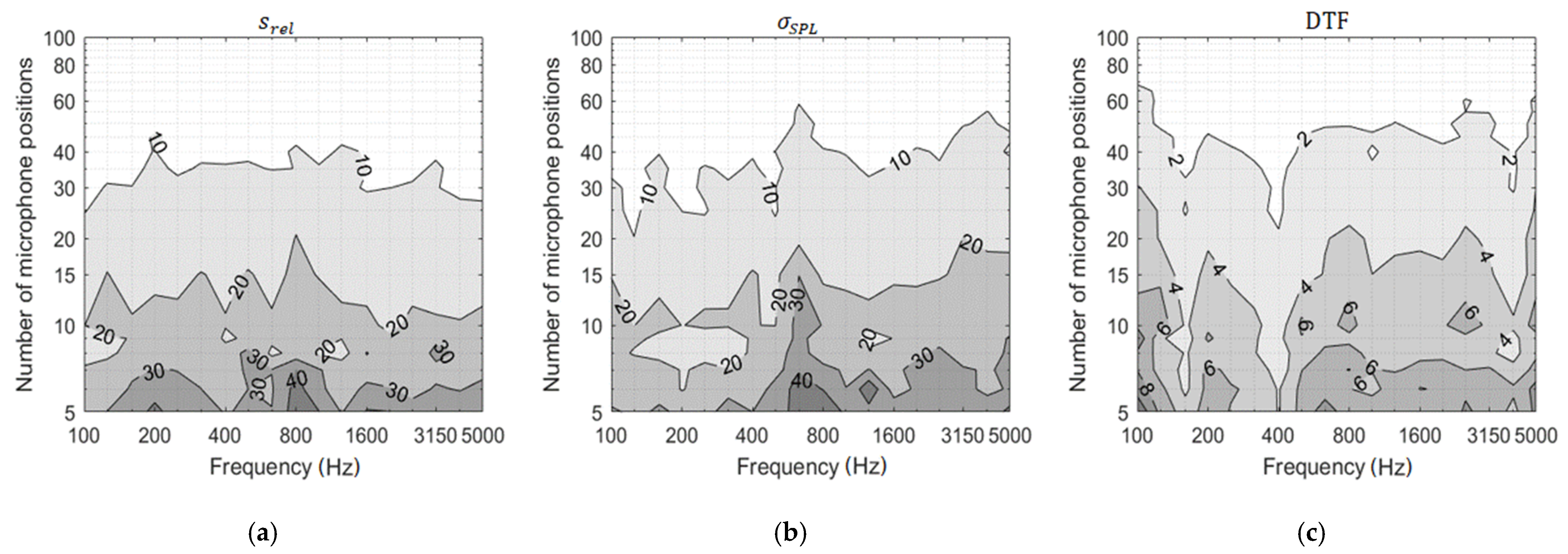
3.2. The Effects of the Number of Measurement Positions on Diffuseness Metrics
4. Conclusions
Author Contributions
Funding
Conflicts of Interest
References
- ASTM International. ASTM C423-17. In Standard Test Method for Sound Absorption and Sound Absorption Coefficients by the Reverberation Room Method; ASTM International: West Conshohocken, PA, USA, 2017. [Google Scholar] [CrossRef]
- International Organization for Standardization. ISO 354:2003. In Measurement of Sound Absorption in a Reverberation Room; International Organization for Standardization: Geneva, Switzerland, 2003. [Google Scholar]
- Joyce, W.B. Exact effect of surface roughness on the reverberation time of a uniformly absorbing spherical enclosure. J. Acoust. Soc. Am. 1978, 64, 1429–1436. [Google Scholar] [CrossRef]
- Stephenson, U.M. A Rigorous Definition of the Term “Diffuse Sound Field” and a Discussion of Different Reverberation Formulae. In Proceedings of the 22nd International Congree on Acoustics, Buenos Aires, Argentina, 5–9 September 2016. [Google Scholar]
- El-Basheer, T.M.; Youssef, R.S.; Mohamed, H.K. NIS method for uncertainty estimation of airborne sound insulation measurement in field. Int. J. Metrol. Qual. Eng. 2017, 8, 19. [Google Scholar] [CrossRef][Green Version]
- Scrosati, C.; Martellotta, F.; Pompoli, F.; Schiavi, A.; Prato, A.; D’Orazio, D.; Garai, M.; Granzotto, N.; Di Bella, A.; Scamoni, F.; et al. Towards more reliable measurements of sound absorption coefficient in reverberation rooms: An Inter-Laboratory Test. Appl. Acoust. 2020, 165, 107298. [Google Scholar] [CrossRef]
- Aida, Y.; Inoue, N.; Sakuma, T. An experimental analysis method for the incident sound field using propagation mode expansion: Study on the incident sound field in the insulation performance measurement for partition walls. Part 1. Jpn. Archit. Rev. 2020, 3, 615–628. [Google Scholar] [CrossRef]
- Neubauer, R.O. Estimation of reverberation time in rectangular rooms with non-uniformly distributed absorption using a modified fitzroy equation. Build. Acoust. 2001, 8, 115–137. [Google Scholar] [CrossRef]
- Hanyu, T.; Hoshi, K. Relationship between reflected sound density and mean free path in consideration of room shape complexity. Acoust. Sci. Technol. 2012, 33, 197–199. [Google Scholar] [CrossRef][Green Version]
- Toyoda, E.; Sakamoto, S.; Tachibana, H. Effects of room shape and diffusing treatment on the measurement of sound absorption coefficient in a reverberation room. Acoust. Sci. Technol. 2004, 25, 255–266. [Google Scholar] [CrossRef]
- Bartel, T.W.; Magrab, E.B. Studies on the spatial variation of decaying sound fields. J. Acoust. Soc. Am. 1978, 63, 1841–1850. [Google Scholar] [CrossRef]
- Davy, J.L.; Dunn, I.P. The effect of moving microphones and rotating diffusers on the variance of decay rate. Appl. Acoust. 1988, 24, 1–14. [Google Scholar] [CrossRef]
- Wang, S.; Zhong, J.; Qiu, X.; Burnett, I. A note on using panel diffusers to improve sound field diffusivity in reverberation rooms below 100 Hz. Appl. Acoust. 2020, 169, 107471. [Google Scholar] [CrossRef]
- Hanyu, T.; Hoshi, K.; Nakakita, T. Assessment of sound diffusion in rooms for both time and frequency domain by using a decay-cancelled impulse response. In Proceedings of the Euronoise 2018, Crete, Greece, 27–31 May 2018; pp. 2011–2018. [Google Scholar]
- Jeong, C.-H. Kurtosis of room impulse responses as a diffuseness measure for reverberation chambers. J. Acoust. Soc. Am. 2016, 139, 2833–2841. [Google Scholar] [CrossRef]
- Nolan, M.; Fernandez-Grande, E.; Brunskog, J.; Jeong, C.-H. A wavenumber approach to quantifying the isotropy of the sound field in reverberant spaces. J. Acoust. Soc. Am. 2018, 143, 2514–2526. [Google Scholar] [CrossRef]
- Lautenbach, M.R.; Vercammen, M.L. Can we use the standard deviation of the reverberation time to describe diffusion in a reverberation chamber? In Proceedings of the ICA 2013, Montreal, QC, Canada, 2–7 June 2013; pp. 2071–2074. [Google Scholar]
- Jeong, C.H. Diffuse sound field: Challenges and misconceptions. In Proceedings of the 45th International Congress and Exposition on Noise Control Engineering, INTER-NOISE 2016, Hamburg, Germany, 21–24 August 2016; pp. 1015–1021. [Google Scholar]
- ASTM International. ASTM International. ASTM E90-09(2016). In Standard Test Method for Laboratory Measurement of Airborne Sound Transmission Loss of Building Partitions and Elements; ASTM International: West Conshohocken, PA, USA, 2016. [Google Scholar] [CrossRef]
- Bradley, D.T.; Müller-Trapet, M.; Adelgren, J.; Vorländer, M. Effect of boundary diffusers in a reverberation chamber: Standardized diffuse field quantifiers. J. Acoust. Soc. Am. 2014, 135, 1898–1906. [Google Scholar] [CrossRef]
- Hanyu, T. Analysis method for estimating diffuseness of sound fields by using decay-cancelled impulse response. Build. Acoust. 2014, 21, 125–134. [Google Scholar] [CrossRef]
- Vallis, J.; Hayne, M.; Mee, D.; Devereux, R.; Steel, A. Improving sound diffusion in a reverberation chamber. In Proceedings of the Acoustics 2015, Hunter Valley, Australia, 15–18 November 2015. [Google Scholar]
- Jeon, J.Y.; Jang, H.S.; Kim, Y.H.; Vorländer, M. Influence of wall scattering on the early fine structures of measured room impulse responses. J. Acoust. Soc. Am. 2015, 137, 1108–1116. [Google Scholar] [CrossRef] [PubMed]
- Prislan, R.; Brunskog, J.; Jacobsen, F.; Jeong, C.-H. An objective measure for the sensitivity of room impulse response and its link to a diffuse sound field. J. Acoust. Soc. Am. 2014, 136, 1654–1665. [Google Scholar] [CrossRef] [PubMed]
- Lokki, T. Diffuseness and intensity analysis of spatial impulse responses. J. Acoust. Soc. Am. 2008, 123, 3908. [Google Scholar] [CrossRef]
- Gover, B.N.; Ryan, J.G.; Stinson, M.R. Measurements of directional properties of reverberant sound fields in rooms using a spherical microphone array. J. Acoust. Soc. Am. 2004, 116, 2138–2148. [Google Scholar] [CrossRef]
- Epain, N.; Jin, C.T. Spherical Harmonic Signal Covariance and Sound Field Diffuseness. IEEE ACM Trans. Audio Speech Lang. Process. 2016, 24, 1796–1807. [Google Scholar] [CrossRef]
- Rafaely, B.; Weiss, B.; Bachmat, E. Spatial aliasing in spherical microphone arrays. IEEE Trans. Signal Process. 2007, 55, 1003–1010. [Google Scholar] [CrossRef]
- Davy, J.L. The variation of decay rates in reverberation room. Acustica 1979, 43, 12–24. [Google Scholar]
- Bodlund, K. Statistical characteristics of some standard reverberant sound field measurements. J. Sound Vib. 1976, 45, 539–557. [Google Scholar] [CrossRef]
- Lubman, D. Spatial averaging in sound power measurements. J. Sound Vib. 1971, 16, 43–58. [Google Scholar] [CrossRef]
- Tichy, J.; Baade, P.K. Effect of rotating diffusers and sampling techniques on sound-pressure averaging in reverberation rooms. J. Acoust. Soc. Am. 1974, 56, 137–143. [Google Scholar] [CrossRef]
- Schroeder, M.R. Spatial Averaging in a Diffuse Sound Field and the Equivalent Number of Independent Measurements. J. Acoust. Soc. Am. 1969, 46, 534. [Google Scholar] [CrossRef]
- Warnock, A.C.C. Some practical aspects of absorption measurements in reverberation rooms. J. Acoust. Soc. Am. 1983, 74, 1422–1432. [Google Scholar] [CrossRef]
- Müller-Trapet, M.; Vorländer, M. Uncertainty analysis of standardized measurements of random-incidence absorption and scattering coefficients. J. Acoust. Soc. Am. 2015, 137, 63–74. [Google Scholar] [CrossRef] [PubMed]
- Elements, C.; Drilled, U.; Cores, C.; Specimens, C.C.; Concrete, H.; Statements, B. Astm E2235−2020. ASTM Int. 2012, 08, 5–12. [Google Scholar] [CrossRef]
- The Acoustical Society of America. ANSI/ASA S1.26-2014. In Methods for Calculation of the Absorption of Sound by the Atmosphere; The Acoustical Society of America: Melville, NY, USA, 2014. [Google Scholar]
- Schroeder, M.R. New Method of Measuring Reverberation Time. J. Acoust. Soc. Am. 1965, 37, 409–412. [Google Scholar] [CrossRef]


| Diffuseness Condition | Case 1 | Case 2 | Case 3 | Case 4 | Case 5 | Case 6 |
|---|---|---|---|---|---|---|
| Diffuser configuration | Empty room | Two hanging diffusers | Four hanging diffusers | Six hanging diffusers | Rotating diffuser | Rotating & Six hanging diffusers |
| Total diffuser surface area (m2) | 0 | 4.16 | 8.32 | 12.48 | 4.14 | 16.62 |
| Metrics | Freq (Hz) | Number of Measurement Samples | |||||
|---|---|---|---|---|---|---|---|
| 5 | 9 | 12 | 15 | 20 | 24 | ||
| 100 | 26.06% | 18.73% | 15.01% | 9.50% | 8.98% | 7.27% | |
| 1000 | 39.85% | 24.55% | 21.03% | 18.79% | 16.54% | 12.47% | |
| 100 | 34.07% | 21.14% | 17.59% | 14.68% | 12.02% | 7.64% | |
| 1000 | 42.76% | 28.22% | 17.91% | 17.56% | 17.31% | 11.24% | |
| DTF | 100 | 10.54% | 7.94% | 7.31% | 5.10% | 4.45% | 4.29% |
| 1000 | 6.11% | 5.20% | 4.11% | 3.52% | 3.09% | 2.39% | |
Publisher’s Note: MDPI stays neutral with regard to jurisdictional claims in published maps and institutional affiliations. |
© 2021 by the authors. Licensee MDPI, Basel, Switzerland. This article is an open access article distributed under the terms and conditions of the Creative Commons Attribution (CC BY) license (https://creativecommons.org/licenses/by/4.0/).
Share and Cite
Zhang, S.; Lee, J. Diffuseness Quantification in a Reverberation Chamber and Its Variation with Fine-Resolution Measurements. Buildings 2021, 11, 519. https://doi.org/10.3390/buildings11110519
Zhang S, Lee J. Diffuseness Quantification in a Reverberation Chamber and Its Variation with Fine-Resolution Measurements. Buildings. 2021; 11(11):519. https://doi.org/10.3390/buildings11110519
Chicago/Turabian StyleZhang, Shuying, and Joonhee Lee. 2021. "Diffuseness Quantification in a Reverberation Chamber and Its Variation with Fine-Resolution Measurements" Buildings 11, no. 11: 519. https://doi.org/10.3390/buildings11110519
APA StyleZhang, S., & Lee, J. (2021). Diffuseness Quantification in a Reverberation Chamber and Its Variation with Fine-Resolution Measurements. Buildings, 11(11), 519. https://doi.org/10.3390/buildings11110519