The Influence of Different Scattering Algorithms on Room Acoustic Simulations in Rectangular Rooms

Abstract

Raytracing is a widespread tool for room acoustic simulations, and one of its main advantages is the inclusion of surface scattering. Although surface scattering has been acknowledged as a central aspect of accurate raytracing simulations for many years, there is ongoing research into its effects and how to implement it better. This study evaluates three different algorithms for surface scattering in raytracers, referred to as on–off scattering, perturbation scattering, and diffuse field scattering. Their theoretical foundation is discussed, and the physical accuracy of the resulting simulations is evaluated by comparing simulated room acoustic parameters to measurements. It is found that the choice of surface scattering algorithm has a significant impact on the simulation outcomes, both in terms of physical accuracy and in terms of usability. Additionally, there are differences in the parametrization of surface scattering depending on the algorithm chosen. Of the three tested algorithms, the most commonly used algorithm (on–off scattering) seems to have the best properties for simulations.

1. Introduction

Raytracing and other geometrical acoustics (GA) techniques have been some of the most popular sound simulation tools for decades [1,2], after first making their appearance in the 1960s [3]. In the early 1990s, the necessity to account for surface scattering in such models became an established fact [4,5,6]. Although the importance of surface scattering was acknowledged already almost 30 years ago, there is no firm consensus on what the best algorithm for scattering in raytracers is. Software based on GA techniques exist in several iterations, such as ODEON [7], CATT acoustics [8], RAMSETE [9] or RAVEN [10], and there are significant differences in how they implement scattering. In addition, several alternatives are typically presented in overviews [2,11,12]. Furthermore, there is still research into what effects the scattering coefficient has on room acoustic parameters using different scattering algorithms [13,14]. This study aims to shed new light on the differences between various scattering algorithms by isolating their effects and evaluating their functionality from new perspectives.

Raytracing as a concept defines both an underlying model for the acoustic field and the simulation tool used to estimate the predictions made by the model. A brief introduction is made here, and more detailed descriptions can be found in many textbooks [1,2,12]. The basic modeling assumption in raytracers is that the acoustic energy emitted from a sound source can be accurately modeled using an infinite set of acoustic particles, or rays, which follow plane wave propagation laws. The rays carry acoustic energy which is decreased by surface absorption or attenuation in the medium, and they typically carry no phase information. By the plane wave model, they are reflected by surfaces in the specular (mirror-like) direction. This model is approximately valid for frequency ranges where the wavelength is significantly smaller than the dimensions of the enclosure, and modal effects are not dominant. The Schröder frequency [15] can be used as a lower limit for when these assumptions might be valid. The acoustic response predicted by this model is calculated by a Monte Carlo simulation, where a random, finite subset of acoustic ray paths are sampled and used as an estimate of the full response. If enough rays are used in the calculation, the calculated response will not vary significantly due to random fluctuations and be very close to the response predicted by the underlying model.

Within this framework, surface scattering can be defined using the suggestion by Morse and Ingard [16]. By this definition, surface scattering is the discrepancy between the ideal reflection of a plane wave from a plane, rigid surface, and the real reflected wave. Due to the modeling assumptions in raytracers, the ideal plane wave reflection is easily defined as the specular reflection, adjusted for the energy absorption by the surface. Models for surface scattering should then aim to compensate for the discrepancy between this model and a more accurate model for the distribution of reflected energy.

As there are variations in the terminology used to discuss surface scattering, a few explanations and motivations for the terms used in this study are provided. The terms diffuse reflection, diffusion, and scattering reflection are all used in the context of surface scattering and raytracing, sometimes more or less interchangeably. In this study, the term scattering reflection is preferred and refers to any reflection that deviates from the ideal plane wave prediction (in the raytracer case, the specular reflection). The term diffusion refers to processes which lead to a more diffuse sound field, i.e., a more uniform distribution of acoustic energy [1]. The term diffuse reflection is not used in the sequel.

There are several effects that may cause reflected acoustic energy to deviate from the specular prediction. In raytracing, the plane wave, energetic model is itself an approximation of sound propagation from a point source and may be inaccurate. In general, if the acoustic ray has travelled a distance r, such that $kr\gg 1$, where k is the wavenumber, the approximation is acceptable [1]. Other sources of scattering may be impedance variations across a surface [1]. Surface elements may be excited and re-radiate acoustic energy [16] in a way that is not accounted for in the rigid surface model. Finally, rough surfaces may introduce scattering by spatial dispersion, temporal dispersion due to unequal path lengths, or edge effects such as diffraction [1,2,12]. All these phenomena may cause the real distribution of reflected energy to deviate from the specularly reflected ray model in the basic raytracer.

Raytracers generally approach scattering reflections by formulating an alternative model for a ray’s energy distribution after reflection. A scattering algorithm is developed based on this model, and the algorithm’s physical accuracy is thus determined by the accuracy of the underlying model. However, selecting a model depends on more factors than physical accuracy. It must also be possible to adapt the mathematical model to raytracers, either by allowing for straight-forward calculations in a different framework or by being appropriate for continued raytracing. Although there are some examples where the first of these options have been implemented [4,5], the second option is more frequently described in the literature [1,2,11,12]. Continued raytracing requires that the model for the reflected energy can be discretized into acoustic particles or rays, which follow plane wave propagation laws. Such models may be constructed based on solutions to the wave equation for that particular surface (which can take all the phenomena discussed above into account); by using a more simplified but specialized model; or by using a general model, such as a Lambertian distribution. When a raytracing-ready model for the energy distribution has been established, the raytracing simulation may continue by sampling the distribution in the same way that the acoustic energy emitted from the sound source is sampled. In addition to technical limitations, the choice of model should lead to a scattering algorithm that is easy and efficient to use. In all, this has led to the Lambertian distribution being the most popular basis for mathematical models of the energy distribution after scattered reflections [2,11,12].

There are two standard coefficients that aim to quantify surface scattering from real surfaces. These are the directional diffusion coefficient defined in ISO 17497-2 [17] and the random-incidence scattering coefficient defined in ISO 17497-1 [18]. The directional diffusion coefficient measures the similarity between the distribution of the reflected energy and a Lambertian distribution. The random-incidence scattering coefficient measures how much of the incident energy is reflected in a direction other than the specular direction when the incident energy is randomly distributed in space. A more detailed description of the two coefficients can be found in [19]. Although these two coefficients describe aspects of the energy distribution after reflection, they are not by themselves enough to formulate a complete scattering algorithm for raytracers. They may however be useful as tools to evaluate existing models or as input values for parametric models. In raytracers in general, it is often difficult but important to find the appropriate material parameters [20,21,22] and the relevance of standard coefficients as input parameters should be considered in the choice of scattering algorithm.

The variations in terminology, models, and standards show a need for more research into surface scattering and how it should be implemented in raytracers. Several papers in recent years examine the effects on simulated room acoustic parameters as the scattering parameter varies and has found that changing the scattering parameter has different effects in different spaces [13] and for different algorithms [14]. A deeper understanding of these results can be achieved by further discussing the physical interpretations of increasing or decreasing the scattering coefficient, and by isolating the effects of different scattering algorithms. These are both goals of the study presented in this paper.

This study describes and evaluates three different raytracing scattering algorithms based on their physical accuracy, simulation speed, and usability. Raytracers are popular partly because they are fast and easy to use, and it is thus important that the scattering algorithms introduced do not violate any of those properties. In order to evaluate the usability of the algorithms, their predictability and sensitivity to parameter errors are reviewed. This study also implements the three scattering algorithms within the framework of one raytracer, isolating the influence of the scattering algorithm itself and separating this study from previous research [5,14].

In this paper, the three scattering algorithms are firstly presented. Then, the methods used for comparing them are explained more in detail, and finally the results of the evaluation are presented and discussed.

2. The Algorithms Implemented in This Study

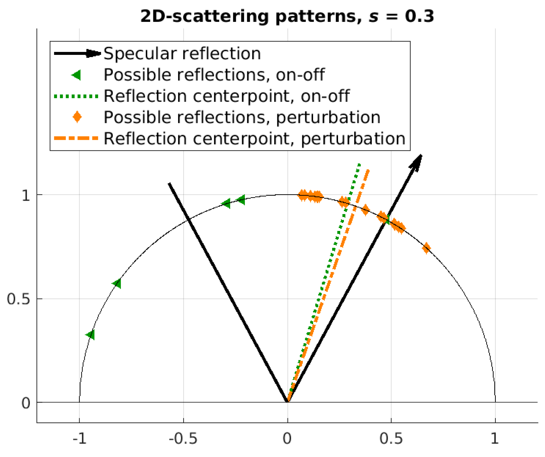
In this section, the three scattering algorithms subject to the study are described. The three algorithms are herein referred to as on–off scattering, perturbation scattering, and the diffuse field algorithm. They are based on three different models for the distribution of energy after a scattering reflection. The on–off scattering and perturbation scattering algorithms are implemented entirely within the raytracing framework, whereas the diffuse field algorithm uses external calculations for parts of the simulation. The reasons for these discrepancies and their implications are discussed. A schematic image of the properties of on–off and perturbation scattering is shown in Figure 1.

2.1. On–Off Scattering

The algorithm herein referred to as on–off scattering is possibly the most common way of implementing surface scattering in raytracers, and it is described in several sources [1,11,12]. It is related to the random-incidence scattering coefficient defined in ISO 17497-1 [18] and uses a Lambertian distribution for the scattered energy.

In the underlying mathematical model, the acoustic energy reflected from a surface consists of a combination of energy reflected specularly and energy scattered according to a Lambertian distribution. The ratio of energy that is scattered is described by a value $s_o\in [0,1]$, called the on–off scattering parameter. All remaining energy is reflected in the specular direction. The value of $s_o$ needs to be defined for each surface separately.

This model is easy to adapt to an algorithm suitable for raytracing simulations. For each ray that hits a surface, it is reflected either in the specular direction or in a random direction generated from a Lambertian distribution. The choice of whether a ray should be reflected specularly or randomly is made so that approximately $s_o$ of all rays intersecting this surface are scattered, which ensures that also a ratio $s_o$ of the total energy incident on this surface is reflected according to the Lambertian distribution. An example of the pattern of reflection directions for $s_o=0.3$ is shown in Figure 1. The name used for the algorithm comes from the on–off behavior for each ray.

The parameter $s_o$ easily relates to the random-incidence scattering coefficient, as defined in the standards [18,19]. The random-incidence scattering coefficient $s_{\mathrm{ISO}}$ measures the ratio of the total reflected energy that is not reflected in the specular direction. A ratio of $1-s_{\mathrm{ISO}}$ is consequently reflected in the specular direction. In the on–off scattering algorithm, $1-s_o$ of the acoustic energy is reflected in the specular direction and in this way $s_o$ and $s_{\mathrm{ISO}}$ are similar. However, there are still differences in the underlying model. When measuring the random-incidence scattering coefficients, no information is obtained regarding the distribution of the energy which is scattered. In contrast, the on–off scattering algorithm uses a Lambertian model for this energy. The Lambertian distribution is a reasonable best guess but cannot be assumed to be generally valid, and some care should be taken before using $s_{\mathrm{ISO}}$ as the on–off scattering parameter.

2.2. Perturbation Scattering

Similarly to on–off scattering, perturbation scattering is implemented entirely within the raytracing framework and parametrized by a single value. It is commonly presented as an alternative to the on–off scattering algorithm [11,12] but does not seem to be as frequently used.

In the mathematical model underlying perturbation scattering, acoustic energy after a scattering reflection forms a cone around the specular direction. The cone’s width is determined by the perturbation scattering parameter, $s_p\in [0,1]$. The larger the parameter, the wider the cone. For $s_p=1$ the distribution defined by the perturbation scattering algorithm will coincide with the Lambertian distribution.

Similarly to on–off scattering, this model is very suitable for raytracing simulations. As a ray intersects a surface, it is reflected in a direction within the cone. The direction is determined by applying a random perturbation (hence the name perturbation scattering) to the direction of specular reflection. The perturbation is generated from a Lambertian distribution and scaled by the perturbation scattering parameter $s_p$. The direction of the reflected ray $d_r$ can thus be described as $d_r=(1-s_p)d_s+s_p{d}_p$, where $d_s$ is the specular direction and $d_p$ is the random perturbation. An example of the pattern of reflections for $s_p=0.3$ is shown in Figure 1.

The perturbation scattering parameter $s_p$ is distinct from the random-incidence scattering coefficient $s_{\mathrm{ISO}}$. The standard random-incidence scattering coefficient defines how much of the reflected energy is directed away from the specular direction, whereas the perturbation scattering parameter regulates how much the reflected energy in general deviates from the specular direction. This random-incidence scattering coefficient can consequently not be assumed to be appropriate for use as perturbation scattering parameter.

2.3. The Diffuse Field Algorithm

The diffuse field algorithm differs from both on–off scattering and perturbation scattering in that it does not rely entirely on raytracing. Although these types of algorithms are less common, there are some previous implementations [4,23]. Similarly to the on–off and perturbation scattering algorithms, the diffuse field algorithm is parametrized using a single value $s_d\in [0,1]$, the diffuse field scattering parameter.

The mathematical model for the diffuse field algorithm relies on the concept of a diffuse acoustic field and interprets surface scattering as an aspect of diffusion. As a sound wave is reflected from a surface, it is assumed that the reflected energy is partly reflected according to the plane wave assumption and partly converted into “diffuse energy” and added to the diffuse field. Energy in the diffuse field is assumed to be uniformly distributed within the volume [1]. The plane-wave segment of the model is easily implemented within a raytracer, and the propagation paths found in this way coincides with statistical implementations of image source models. In each reflection, a ray’s energy is adjusted according to surface absorption and the diffuse field scattering parameter, so that $e_r=e_i(1-\alpha )(1-s_d)$, where $e_r$ is the energy carried by the reflected ray, $e_i$ is the energy of the incident ray, $\alpha$ is the surface’s absorption parameter and $s_d$ the diffuse field scattering parameter. The energy added to the diffuse field, $e_d$ is determined by $e_d=e_i(1-\alpha )s_d$.

The energy transferred to the diffuse field is recorded separately and assumed to be evenly distributed in the entire volume quickly. After that, it decays exponentially. According to theoretical models for diffuse acoustic fields, the energy from the diffuse field that is received at the detector $E_d$ can be calculated as

$$\begin{array}{c}\hfill E_d=A_d\frac{c}{4}w,\end{array}$$

(1)

where $A_d$ is the total surface area of the detector, c is the speed of sound and w is the energy density [1]. The energy density is estimated as $w=\frac{E_{\mathrm{diff}}}{V}$, where $E_{\mathrm{diff}}$ is the total energy in the diffuse field and V is the volume of the simulated space. The energy contained within the diffuse field varies over time, as it decays exponentially and more energy is added from surface scattering.

A complication with this model is that energy may be detected in a non-physically short amount of time. As soon as energy is transferred to the diffuse field, no matter where the reflection causing it occurs, it can be detected anywhere in the simulated space. To counteract this, a method suggested by Lam is implemented [23]. Energy is added to the diffuse field after a delay corresponding to the time needed to travel the mean free path.

The decay rate of the diffuse field may be determined in several ways, for example by using theoretical models such as Sabine’s or Eyring’s formulae. In this case, it is estimated using the raytracer. Several rays are emitted into the modeled space and are reflected in a random direction at each surface. After a certain number of reflections, they are assumed to be well-mixed and approximately uniformly distributed, thus emulating the diffuse field. This step is called a burn-in. After this time, the rays start losing energy according to the absorption parameters of the modeled space and air absorption. The time until the energy of each ray decreases below some pre-defined threshold is recorded and used to estimate the decay rate of the diffuse field. Since the decay rate of the diffuse field is constant for the entire acoustic volume, this step is only needed once for any number of simulations in a given space. In addition, the total number of rays needed is relatively small for two reasons. Firstly, only one parameter needs to be estimated. Secondly, the result for each ray is recorded separately, which allows for statistical outlier detection that stabilizes the estimate. In this study, the decay rate is estimated using 10% of the total number of rays, and the remaining rays are used for the traditional raytracing simulation.

After the raytracing simulation, the results from simulations using the diffuse field algorithm thus consist of three data sets. (1) A reflectogram showing the detected energy from the traditional raytracing simulation; (2) Decay data obtained from the diffuse field decay rate estimation step; and (3) Data showing how much energy is transferred to the diffuse field in each time segment. The energy contained in the diffuse field is determined for each time segment using datasets 2 and 3. Of this energy, the ratio determined by Equation (1) is added to the reflectogram to obtain a full energetic impulse response. This step is performed externally and considered part of the post processing.

In the diffuse field algorithm, surface scattering is parametrized using a single value: The diffuse field scattering parameter $s_d$. It can be interpreted as the amount of diffusion caused by reflection in a given surface. However, since the concept of a diffuse field itself is an idealization of real sound fields, it is unclear whether this is a physical property that can be measured. The diffuse field scattering parameter is not related to either the random-incidence scattering coefficient or the directional diffusion coefficient (defined in ISO 17497-1 and 2, respectively [17,18]).

The diffuse field algorithm and its underlying model can be interpreted as a combination of an image source model and a diffuse field model. With this interpretation, the diffuse field scattering parameter acts akin to a weighting coefficient, determining the relative influences of the diffuse field and image source models in the simulation.

2.4. Differences and Similarities between the Algorithms

The on–off scattering algorithm and the perturbation scattering algorithm are very similar in many aspects. From a practical standpoint they only differ in the directions in which rays are reflected after hitting a surface. These types of algorithms can easily be constructed by finding new distributions for the reflected rays, possibly based on more complex or physically-based models of various surfaces. This is a frequently suggested modification, which is theorized to improve the accuracy of the simulation as a whole [11,12]. A full comparison of on–off and perturbation scattering may shed light on the impact of the model for the reflected energy, and show whether better models can be expected to lead to significant improvement.

The diffuse field algorithm, on the other hand, is quite dissimilar to the previous two algorithms. The theoretical model it is based on is different in itself, and it relies partly on numerical calculations for parts of the simulations. The numerical calculations may mean that the algorithm is less affected by random noise and thus more reliable. Furthermore, if the calculations are sufficiently optimized, it may be faster to use than running a full raytracing simulation even considering the time needed to determine the diffuse field decay rate. Comparing the diffuse field scattering algorithm to the on-off and perturbation scattering algorithms is expected to help show the differences between hybrid methods and fully raytracing-based algorithms.

All three algorithms described are parametrized using a single scattering parameter, but the physical and numerical significance of this parameter differs between them. Consequently, it cannot be expected that a surface should have the same on-off, perturbation, and diffuse field scattering parameters. Of the three, only the on–off scattering parameter is easily related to one of the standardized coefficients, namely the random-incidence scattering coefficient [18]. For the diffuse field algorithm, in particular, the relation between its scattering parameter and physical properties of surface scattering is hard to define. Instead, it acts as something of a weighting factor between two models for sound propagation, the energetic plane wave model used in raytracers and the purely diffuse field model.

3. Evaluating the Scattering Algorithms

As mentioned in the introduction, the scattering algorithms examined in this study are evaluated in three different aspects:

• Physical accuracy;
• Simulation speed;
• Usability.

In this section, the methodology used for comparing algorithms is presented and discussed.

3.1. Physical Accuracy

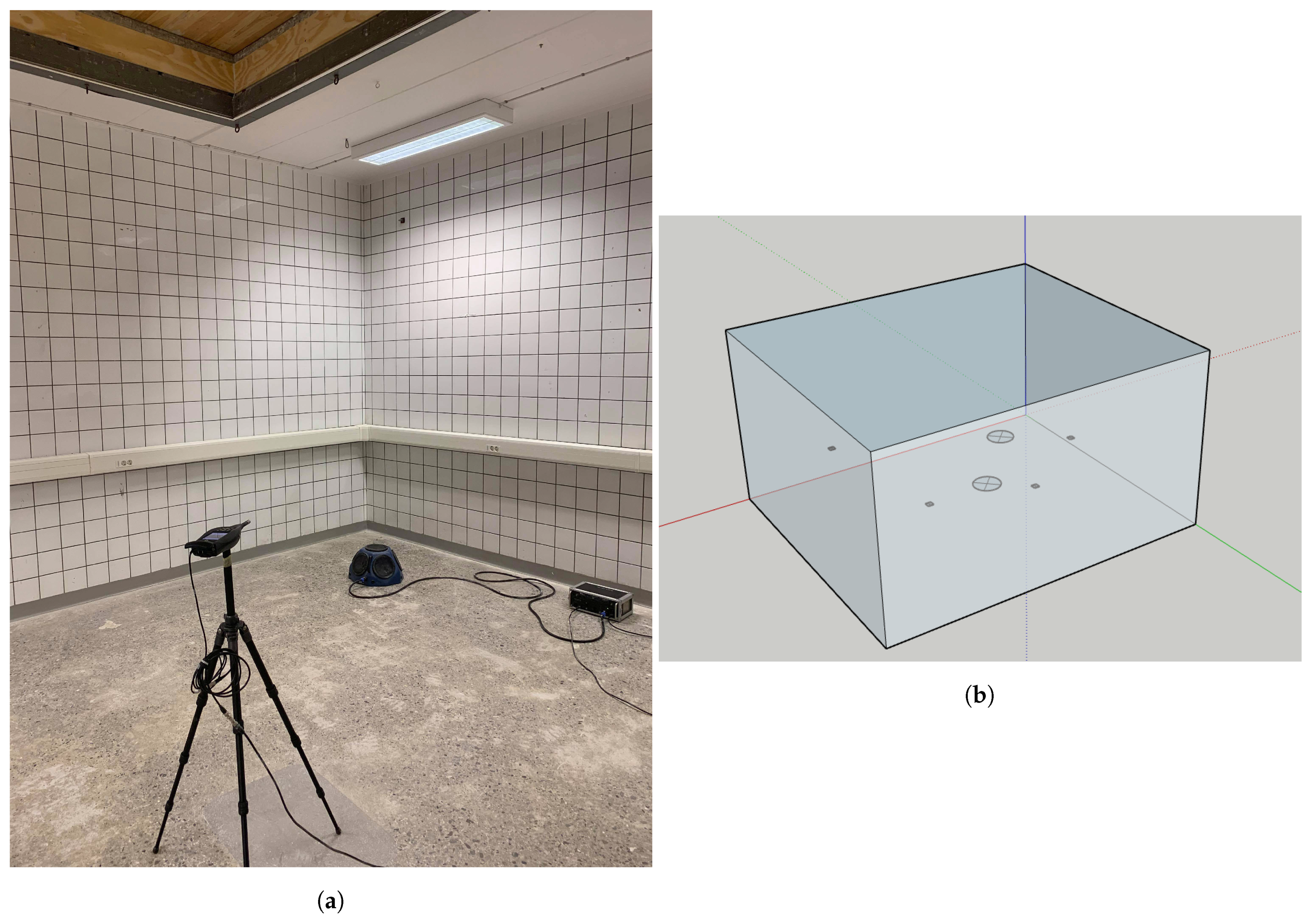
The physical accuracy of the scattering algorithms was evaluated by comparison between simulations and measurements. Measurements were carried out in the lower chamber of the impact sound lab in the Division of Engineering Acoustics, LTH (Lund University), shown in Figure 2. It has a total volume of approximately 95 ${\mathrm{m}}^3$ and was measured in two conditions. The first condition, herein referred to as case A, is a highly reverberant condition where all surfaces are acoustically hard. The second condition, case B, is similar but has introduced a patch of highly absorptive material in the ceiling. It is expected that the concentrated absorption in case B should correspond to a higher sensitivity to the scattering algorithm and the scattering parameter, whereas case A acts as a useful baseline. Further details on the measurements are presented in Section 4.

Simulations and measurements were compared using three standard room acoustic parameters, reverberation time ($T_{20}$), early decay time (EDT), and speech clarity ($C_{50}$), as defined in [24]. The reverberation time was included as it is a ubiquitous measure often used as a design parameter, and it is thus crucial that simulation software can predict it accurately. The EDT has been shown to be closely related to the perceived reverberation, and it is consequently important that it can be simulated correctly. Finally, clarity for speech or music ($C_{50}$ and $C_{80}$, respectively) is a perceptually important aspect of the sound field. Since the measured space is relatively small and, thus, more likely to be used for speech presentation, it was concluded that $C_{50}$ was more relevant. All three room acoustical parameters were compared using the measured just noticeable difference (JND, as defined in [24]), and values that are within 1 JND are assumed to be perceptually similar.

The simulations were performed using absorption and scattering parameters estimated by several methods. It is a common issue in room acoustic simulations that the material parameters of existing surfaces are unknown [20,21,22] and must be calibrated somehow to achieve a good match between measurements and simulations. Generally, this holds for both scattering parameters and absorption parameters. In this study, it is assumed that the scattering parameter may vary between the algorithms, whereas the absorption parameter corresponds to the sound absorption coefficient as defined in [25] and is the same for all algorithms. Consequently, the scattering parameters were estimated for each of the algorithms individually, as described in Section 4.2, and the absorption parameters were estimated for all algorithms simultaneously using two different methods. The only material for which the absorption coefficient was available was the absorptive material in case B, and table values from the manufacturer were used for this material.

For middle to high frequencies, the tested algorithms themselves were used to calibrate the absorption parameters. Simulations were run for all algorithms using a wide range of scattering parameters, and spatial average room acoustic parameters were extracted. The results from each algorithm were compared to measurements to see if there was any one scattering parameter value for which all room acoustic parameters were within 1 JND of the measurements. When such a value existed for all algorithms, it was assumed that the absorption parameters were sufficiently accurate.

For frequencies 500 Hz and below, a different method for estimating the absorption parameters were used. Since raytracers are known to perform poorly for frequencies below the Schröder frequency, they were not considered appropriate tools for estimating a value corresponding to a physical property. Instead, a mode-based method presented by Meissner [26] was used. This method estimates the EDC for low frequencies in rectangular spaces with hard, reflective walls. Modal damping factors calculated from the specific wall conductances are used to model the energy decay over time by summating over eigenfrequencies. The EDC from Meissner’s calculations was compared to the measured EDC, and the reverberation time was extracted and compared to the measured value. The specific wall conductances were tuned until the calculations were close to the measurements. The absorption coefficients were estimated from the specific wall conductances [15,26] and used as absorption parameters in the simulation.

The algorithms were evaluated both by comparison of spatially averaged room acoustic parameters and based on their ability to predict spatial variations of the sound field. Spatial variations were examined by studying measured room acoustic parameters for each of the positions shown in Figure 2. These were compared to simulated values using the same positions. Ideally, any variations between positions should be similar for both sets of results.

3.2. Simulation Speed

The simulation time for the three algorithms was examined to identify any significant differences between them. In the comparison, only the time used for raytracing has been included, although the diffuse field algorithm requires significantly more external calculations and post processing, increasing the total time consumption. This choice was made since this study focuses on raytracing algorithms in particular.

The time consumption of raytracers generally depends on the number of rays used in the simulation. This, in turn, is governed by the desired level of precision and accuracy. If the number of rays is sufficiently large, the simulation results are consistently very close to the predictions made by the underlying model, whereas too few rays lead to results that may vary significantly between calculations or deviate significantly from the predictions made by the model. How many rays are needed depends on the modeled space [2] including the material parameters and on the algorithm used. In this study, the number of rays needed in each of the three algorithms was evaluated separately. In this way, the time consumption for each algorithm could be measured using the appropriate number of rays.

The sufficient number of rays was determined by reviewing how much the simulation results deviated from the prediction made by the underlying model. This was evaluated by defining the maximum simulation error, $e_{\mathrm{Sim}}$. The $e_{\mathrm{Sim}}$ is the largest deviation between a baseline value and a simulated value for a given number of rays. The baseline value is defined as the average result of a set of simulations with many rays, and is thus close to the value predicted by the underlying model. The $e_{\mathrm{Sim}}$ was defined for each of the room acoustic parameters mentioned in Section 3.1, according to Equation (2).

$$\begin{array}{c}\hfill e_{\mathrm{Sim}}=\underset{p\in P,l\le L}{max}|x_{p,l}-{\overline{x}}_p|,\end{array}$$

(2)

where $x_{p,l}$ is the simulated value of a room acoustic parameter for source and receiver position p and simulation number l. ${\overline{x}}_p$ is the baseline value of the selected room acoustic parameter for that position, and P is the set of all positions. L is the total number of simulations run with that specific number of rays. Note that $e_{\mathrm{Sim}}$ only measures the reliability of the simulation. A small $e_{\mathrm{Sim}}$ indicates that a simulation using this number of rays accurately finds the value predicted by the underlying physical model, not whether that model is accurate or not.

When the $e_{\mathrm{Sim}}$ fell below 1 JND for all three room acoustic parameters and octave bands, it was assumed that the number of rays was sufficiently high for this algorithm. The time consumption for a raytracing simulation using this algorithm and this number of rays was then measured and compared to the other algorithms.

3.3. Usability

Finally, the usability of the three algorithms was examined by studying the variations in simulation outcome for varying input scattering parameters. Three aspects were evaluated: whether small variations in input value leads to small changes in simulation outcome; whether changes in the input parameter have a predictable effect; and whether reasonable input values yield reasonable simulation results.

To evaluate how the simulation results vary based on variations in the scattering parameter, a set of simulations using a range of scattering parameter values were performed. According to previous research, changes in the scattering parameter have a larger impact when its value is small [10,13]. Consequently, a finer resolution of scattering parameter values was used for smaller values. By evaluating the room acoustic parameters for each of the scattering parameter values used, an estimate of the influence of the scattering parameter was obtained.

The results from changing the scattering parameter in the three algorithms can be compared to results from previous research to determine whether they are predictable in the sense of behaving similarly to other algorithms. In general, increased scattering parameter lead to either a decreased reverberation time [10,13] or have no effect on it [14,21]. The discrepancies might be due to differences in the spaces being modelled. Research on relatively small, rectangular spaces found that reverberation decreased [10,13]. For the test space in this study, it is thus expected that increases in the scattering parameter should decrease the reverberation time. Regarding clarity, previous research is again inconclusive but indicate that increased scattering has no significant impact [14] or leads to reduced clarity [21]. However, both these results are produced for relatively complex test spaces, and the results in this study may be different.

Reasonable values for the scattering parameter are obtained from the research above, engineering handbooks for some commercial software [27,28] and table values of the random-incidence scattering coefficient [2,12]. For the surfaces in the test spaces, a reasonable initial value of the mid-frequency scattering parameter is about $0.1$. Using this scattering parameter, the simulation results should be fairly accurate, although it cannot be expected that 0.1 is the ideal value for all algorithms.

4. Method

In this section, the technical details of the research undertaken in this study is presented.

4.1. Measurements

Impulse response measurements were carried out in the test space using the open-source REW (https://www.roomeqwizard.com/, accessed on 29 August 2021) measurement software installed on a laptop connected to an Audio 8 DJ soundcard from Native Instruments (https://www.native-instruments.com/en/, accessed on 29 August 2021). A Bruel&Kjaer amplifier type 2734 (https://www.bksv.com/en/transducers/acoustic/sound-sources/power-amplifier-2734, accessed on 29 August 2021) connected the soundcard to a dodecahedral loudspeaker, which was used as a sound source. The impulse response was recorded using a Bruel&Kjaer Type 2270 Sound Level Meter and Analyzer (https://www.bksv.com/en/instruments/handheld/sound-level-meters/2270-series/type-2270-s, accessed on 29 August 2021) as a microphone. Two source positions and four microphone positions were used, marked in the digital model in Figure 2. Due to technical limitations and the size of the test space, the sound source was located closer to the floor than described in the measurement standards.

Octave band room acoustic parameters for frequencies in the range 125 Hz to 4000 Hz were extracted using the open-source MATLAB package ITA-acoustics [29]. This includes reverberation time $T_{20}$, EDT, and $C_{50}$, as well as the EDC. When applicable, these have been spatially averaged according to the international standard for measurements of these parameters [24].

4.2. Material Parameter Calibration

Meissner’s algorithm [26] for estimation of the EDC was implemented in MATLAB. As mentioned in Section 3, this method is based on a summation of the contributions from the room’s eigenmodes, subject to damping factors determined by the conductance of the walls. Estimates for case A, the space with hard walls, were obtained for octave bands centered on 125 Hz, 250 Hz, and 500 Hz by summation of all the eigenmodes in the corresponding octave bands. The reverberation time $T_{20}$ was extracted from the EDC.

The Meissner algorithm was used to tune the absorption parameter for the three octave bands in question. This was done iteratively. Initial guesses of the specific wall conductances were set to 0.0053 for all surfaces, corresponding to a random incidence absorption coefficient (and, thus, absorption parameter) of 0.04. Then, this value was adjusted for each of the surfaces until the estimates of the reverberation time were within 1 JND, and good visual correspondence between the measured and the calculated spatial mean EDC was obtained. The absorption parameters corresponding to the found conductances are shown in

Table 1. Absorption parameters used in the simulations. The values for the porous absorbers are table values for the random-incidence absorption coefficient, taken from the manufacturer of the product. For bands centered on 125–500 Hz, the absorption parameters are random-incidence absorption coefficients estimated from the conductances used in the Meissner calculations. The remaining values have been estimated by simultaneous tuning for all algorithms, trying to emulate the measurements.

Material	125 Hz	250 Hz	500 Hz	1000 Hz	2000 Hz	4000 Hz
Tiled walls	0.0734	0.056	0.0453	0.04	0.045	0.045
Concrete floor	0.0596	0.0453	0.0453	0.045	0.045	0.045
Ceiling (concrete slab)	0.0665	0.0631	0.0453	0.04	0.04	0.04
Ceiling (porous absorber)	0.25	0.80	0.95	0.95	0.95	0.95

.

For octave bands centered on 1000 Hz and up, absorption parameters were estimated from initial estimates of $\alpha =0.04$ for all surfaces except the porous ceiling in case B. This value was tuned iteratively by adjusting the value for all materials individually and running additional simulations for all algorithms. This process continued until the spatial average room acoustic parameters were approximately within 1 JND of the measurements for all algorithms, according to the method described in Section 4.2. Regarding the porous ceiling, absorption parameters for all frequencies (including 125 Hz–500 Hz) were obtained from table values from the manufacturer. The resulting values are shown in Table 1.

In order to find appropriate scattering parameters, a range of scattering values were tried in simulations with each of the algorithms. Scattering parameters were varied over the range $[0.01,0.99]$, and the tested values are shown in

Table 2. The range of scattering values and number of rays used for simulations. In total, 23 different scattering parameters and 14 different numbers of rays were used.

Scattering Parameters	Number of Rays
0.01	60
0.03	240
0.035	600
0.04	1920
0.045	6000
0.05	18,960
0.055	60,000
0.06	540,000
0.065	600,000
0.07	900,000
0.1	1,200,000
0.13	3,000,000
0.15	4,500,000
0.17	6,000,000
0.2
0.25
0.3
0.35
0.4
0.5
0.7
0.9
0.99

. From these values, the scattering parameter which yielded the best match between measured and simulated room acoustic parameters were chosen as most appropriate. The best match was evaluated by studying the deviation between simulated and measured values, as calculated by

$$\begin{array}{c}\hfill E_{\mathrm{JND}}=\frac{x_{\mathrm{sim}}-x_{\mathrm{meas}}}{1\mathrm{JND}},\end{array}$$

(3)

where x is one of the spatially averaged room acoustic parameters, and the JND corresponding to that measured parameter is used. Values inside the range $[-1,1]$ then indicate that the room acoustic parameter is sufficiently well estimated. Using this expression allows for the simultaneous graphical evaluation of all three room acoustic parameters. The scattering parameters were assumed to be constant for all hard surfaces in the test space. Consequently, they were tuned simultaneously for case A and B.

4.3. Simulations

The three scattering algorithms were implemented within AMRT, an in-house acoustic raytracer at the Division of Engineering Acoustics at LTH, Lund University. The raytracer is based on the NVIDIA OptiX raytracing engine [30], version 5.1. All models include frequency-dependent air absorption corresponding to a temperature of 20 °C and 70% relative humidity [1]. This is a relatively high humidity for an indoor space, but is reasonable for the test space as it is located in a basement with significant air exchange to the external environment. The outside humidity during the measurements was around 80%–90%.

A digital model of the test space in case A (no absorption) and B (localized ceiling absorption) was developed using Trimble SketchUp (www.sketchup.com, accessed on 29 August 2021), shown in Figure 2b. This model was used for simulations.

Several simulations using different parameters were run for each algorithm. Here, a single simulation refers to the calculation of the energetic impulse response for the eight combinations of source and listener positions (shown in Figure 2b), in the six octave bands ranging from 125 Hz to 4000 Hz. Simulations were run using 23 different scattering values in the range $[0.01,0.99]$, shown in Table 2, with 6,000,000 rays. Each simulation was run five times to reduce the effects of random fluctuations. These results were used for calibration of the scattering parameters, as well as evaluation of the physical accuracy and usability of the algorithms.

Additional simulations using the tuned scattering parameters were run to study the time consumption of the algorithms. Five simulations using fourteen different numbers of rays, in the range [60, 6,000,000] (shown in Table 2), were run for each algorithm. These results were used to calculate the maximum simulation error $e_{\mathrm{Sim}}$ and measure the time consumption for each of the algorithms.

5. Results and Analysis

In this section, the results of the measurements and simulations are presented and analyzed based on the methodology presented previously. As an initial step, the measurements are presented, and the calibrated absorption and scattering parameters are presented. Subsequently, results pertaining to physical accuracy, simulation speed, and usability are presented.

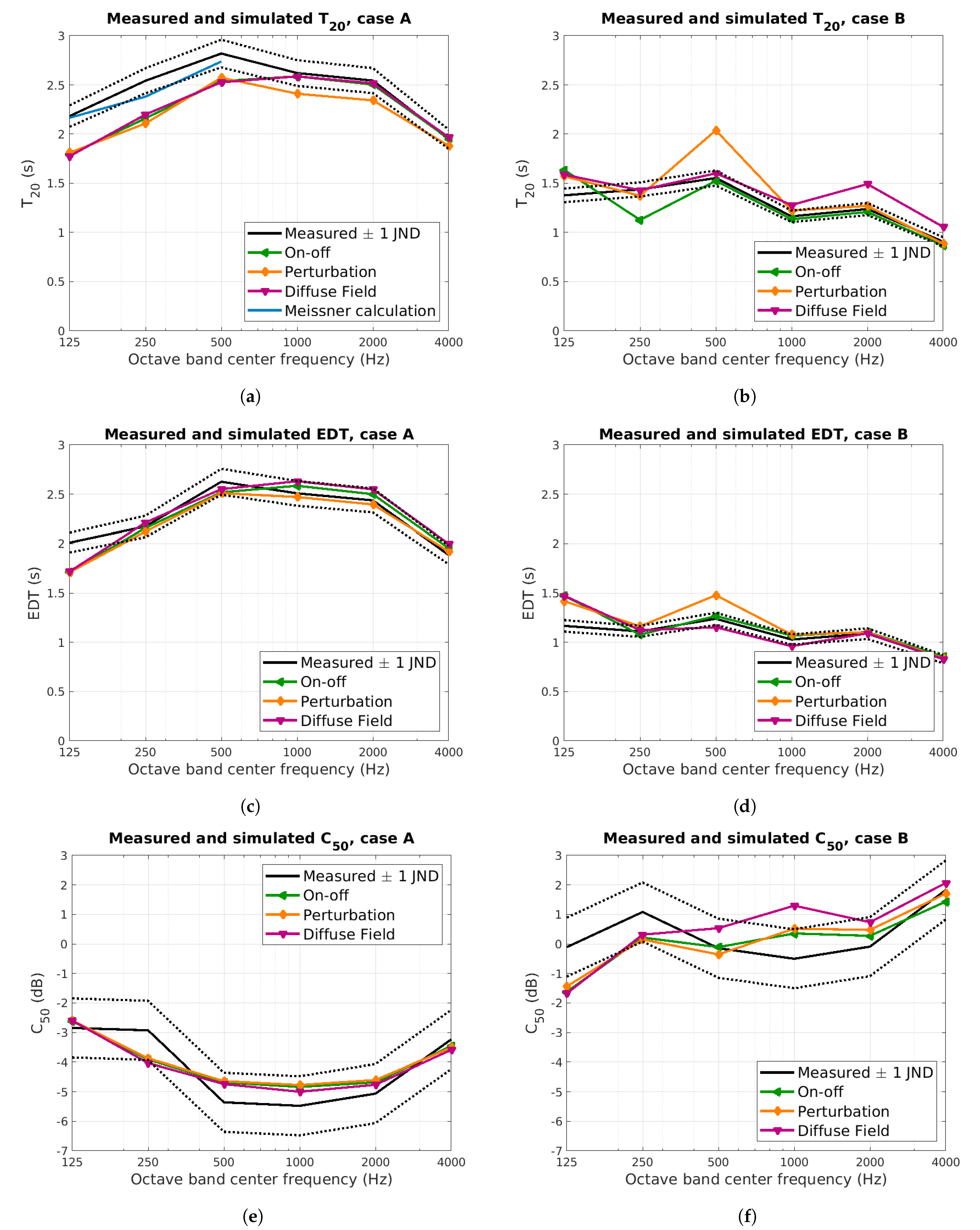
The measured spatially averaged room acoustic parameters are shown in black in Figure 3. In particular, it should be noted that the reverberation time is lower for the lowest frequencies, especially in case A. This is unexpected, as the materials in the space are generally expected to have lower absorption for lower frequencies, which should lead to a longer reverberation time. Although modal effects could lead to decreased reverberation due to cancellation, such effects are not expected to be dominant in the spatial average results. Instead, it is assumed that there is some transmission of low-frequency acoustic energy through the walls and the concrete ceiling. As these results are used to obtain the absorption parameters used in the simulations (shown in Table 1), the absorption parameters are in general higher for low frequencies than what is typically supplied in engineering tables. Overall, the values of the absorption parameters seem consistent with the very hard, mostly reflective surfaces in case A.

The calibrated scattering values used for simulation are shown in

Table 3. Suitable scattering values for the two cases and different algorithms. They have been determined using the method described in Figure 4. Missing values indicate that no scattering value could be found for which the average room acoustic parameters were accurate. Values indicated by ${}^{†}$ are scattering values that outperform other scattering values in the given case, although some room acoustic parameters are outside 1 JND.

		125 Hz	250 Hz	500 Hz	1000 Hz	2000 Hz	4000 Hz
Hard surfaces	On-off	-	-	0.05 ${}^{†}$	0.13	0.1	0.25
	Perturbation	-	0.09 ${}^{†}$	-	0.135 ${}^{†}$	0.12 ${}^{†}$	0.2
	Diffuse Field	-	-	0.03 ${}^{†}$	0.05 ${}^{†}$	0.035 ${}^{†}$	0.05 ${}^{†}$
Absorbers	On-off	-	-	0.1	0.1	0.1	0.1
	Perturbation	-	-	0.1	0.1	0.1	0.1
	Diffuse Field	-	-	0.1	0.1	0.1	0.1

${}^{†}$ signifies values that do not fulfill the criteria but outperform other values.

, obtained using the method described in Section 4.2. For the absorbers in case B, it was found that the scattering parameter had no impact on the simulation outcome. Accordingly, they were assigned a constant value. For the remaining surfaces, the optimal scattering parameter was determined by graphical evaluation of the relative deviation from measurements, as determined by Equation (3). Examples of the graphs used are shown in Figure 4. In many cases, there existed a scattering parameter value, such that all room acoustic parameters were estimated sufficiently well. When this is not the case, scattering parameters for which most room acoustic parameters are well-estimated were selected, if available. However, in some cases, no such values could be found. This occurs for low frequencies and for the perturbation and the diffuse field scattering algorithms, and the relevant values are marked in Table 3. Possible explanations for these issues are described in Section 5.1.

As previously discussed, the scattering parameters have no clearly defined physical counterpart, and their “accuracy” is, thus, hard to evaluate. However, some comments can be made regarding how well they correspond to physical measurements of scattering in general and suggested scattering parameters from engineering tables. Firstly, it is noted that the tuned scattering parameters generally increase as the frequency increases for all algorithms except between 1000 Hz and 2000 Hz. Increased scattering with increased frequency is consistent with typical results when scattering is measured [12] and suggested parametrization in commercial software [28,31]. Secondly, the tuned scattering parameters are relatively small, as expected for the smooth surfaces in the test space.

5.1. Physical Accuracy

To evaluate the physical accuracy of the model, the spatially averaged room acoustic parameters are considered, as shown in Figure 3. In most cases, simulation results are within 1 JND for frequencies above 1000 Hz for all room acoustic parameters. However, both the perturbation algorithm and the diffuse field algorithm results deviates from measurements and other simulated values by more than 1 JND in several cases. This coincides with the frequency bands for which the corresponding scattering parameter could not be tuned. The poor results for the diffuse field algorithm in case B is likely explained in part by issues in the underlying modeling assumptions and how they relate to the modeled space. As described in Section 2, the diffuse field algorithm assumes that part of the acoustic field can be accurately modeled using a diffuse field model. When there is a localized patch of absorbent material, as in case B, there is typically a net flow of energy towards the absorbers and the diffuse field model is invalidated. It is reasonable that the scattering algorithm fails when the underlying modeling assumptions are inaccurate.

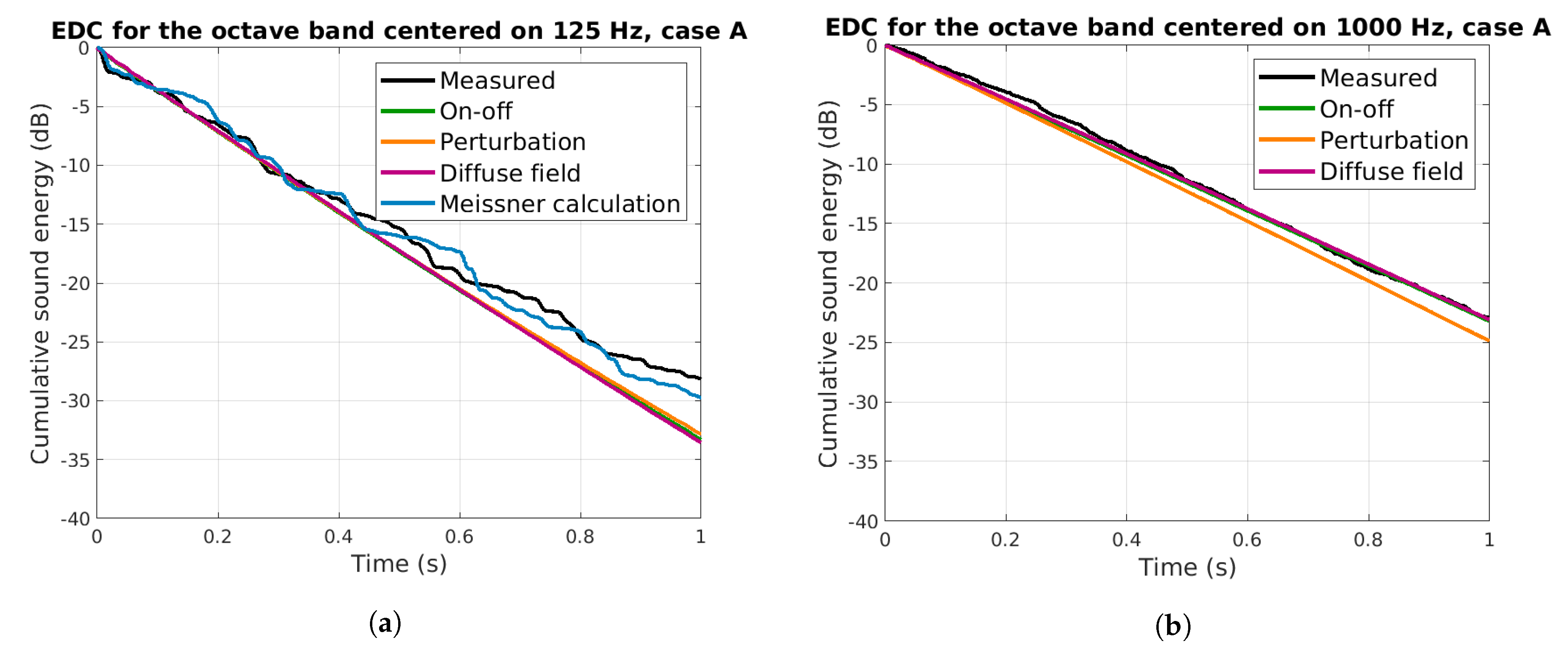
The discrepancy between measurements and simulations for octave bands up to 500 Hz can be explained by the issues in modelling modal behavior in raytracers. The fact that the results from the Meissner calculations, shown in Figure 3a, model the sound field more accurately supports this theory. The difference between low and middle to high frequencies is further illustrated by comparing the EDC, as shown in Figure 5.

There are apparent qualitative differences between the measured EDC for 125 Hz and that for 1000 Hz. In the higher frequency band, the measured EDC is almost linear, whereas the measured EDC for 125 Hz is much more dynamic due to lower modal density. The complex behavior in the low frequency case is emulated quite well by the EDC produced from Meissner’s calculation, although they are not identical. Regarding the raytracer results, however, there are no such qualitative differences between low and high frequency behavior. The EDC is almost linear in both cases.

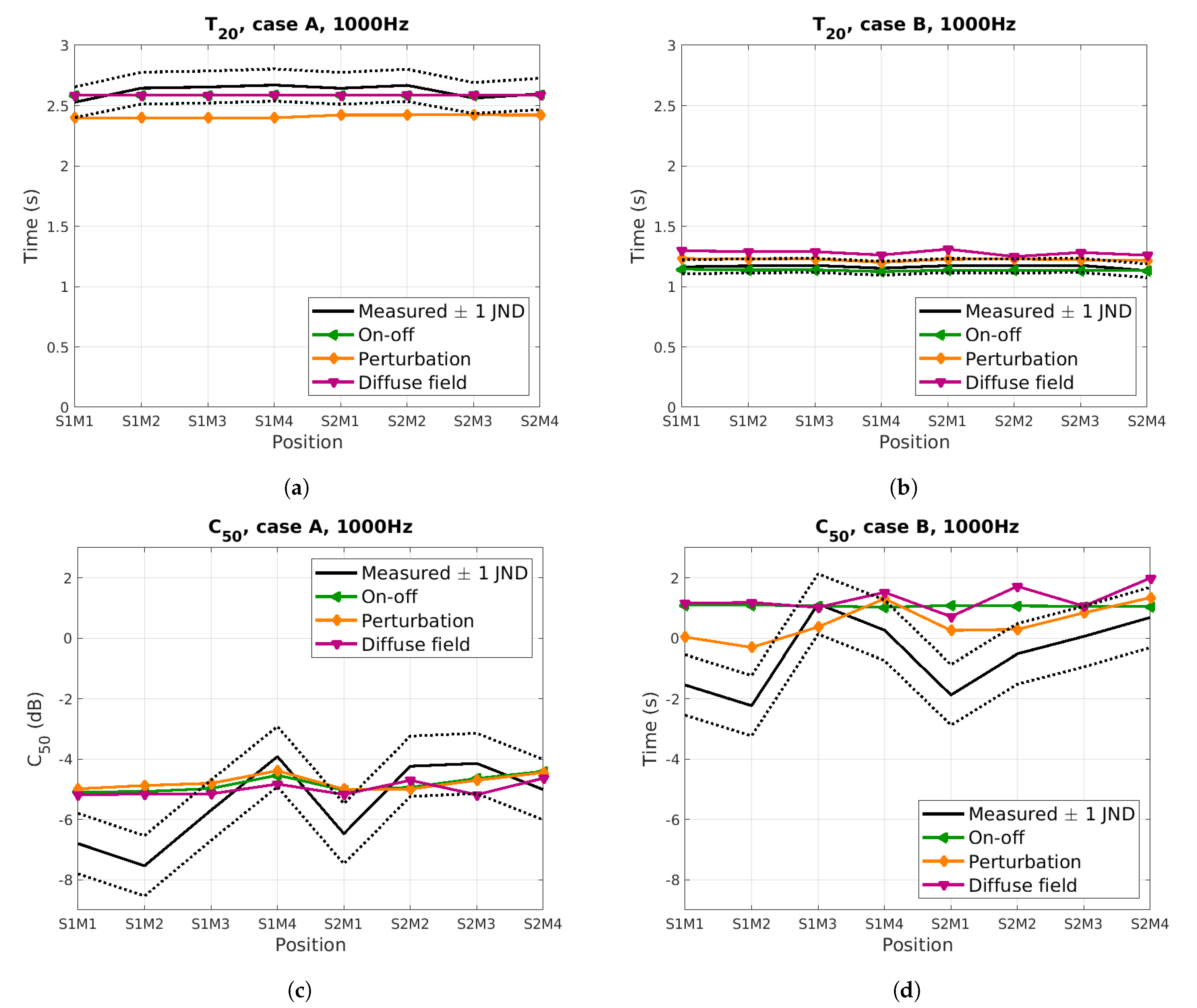
The room acoustic parameters so far have been presented as spatial averages, neglecting any spatial variations. The measured and simulated $T_{20}$ and $C_{50}$ for each position are shown in Figure 6. There is none or minimal spatial variation in the measured reverberation time, and this is replicated in the simulations for all algorithms. In case B, it is again evident that the diffuse field algorithm deviates from the measured value and the values predicted from the other algorithms. However, the deviation is very consistent in size, and the spatial variations are thus similar for all three algorithms.

There are more significant spatial variations in the results for $C_{50}$. This parameter should be more significantly impacted by strong early reflections and thus vary more for different positions. The variations in the measured data are much larger than in the simulated data, although the simulations are mostly within 1 JND of the measurements. There could be several explanations for the discrepancies, including issues both in the measurement process and the simulation process. Measurement noise may lead to random fluctuations in the measured $C_{50}$. On the other hand, the lack of spatial variations in the simulated $C_{50}$ may reflect shortcomings in the simulations. Since the $C_{50}$ depends on early reflections, it can be heavily influenced by any simplifications made in the modeling process. In fact, as the geometric model for the space is so regular, it is quite expected that the simulated data do not show any spatial variations.

Based on the results shown in Figure 6, none of the scattering algorithms tested seems to outperform the others in emulating spatial variations in the measurements.

5.2. Simulation Speed

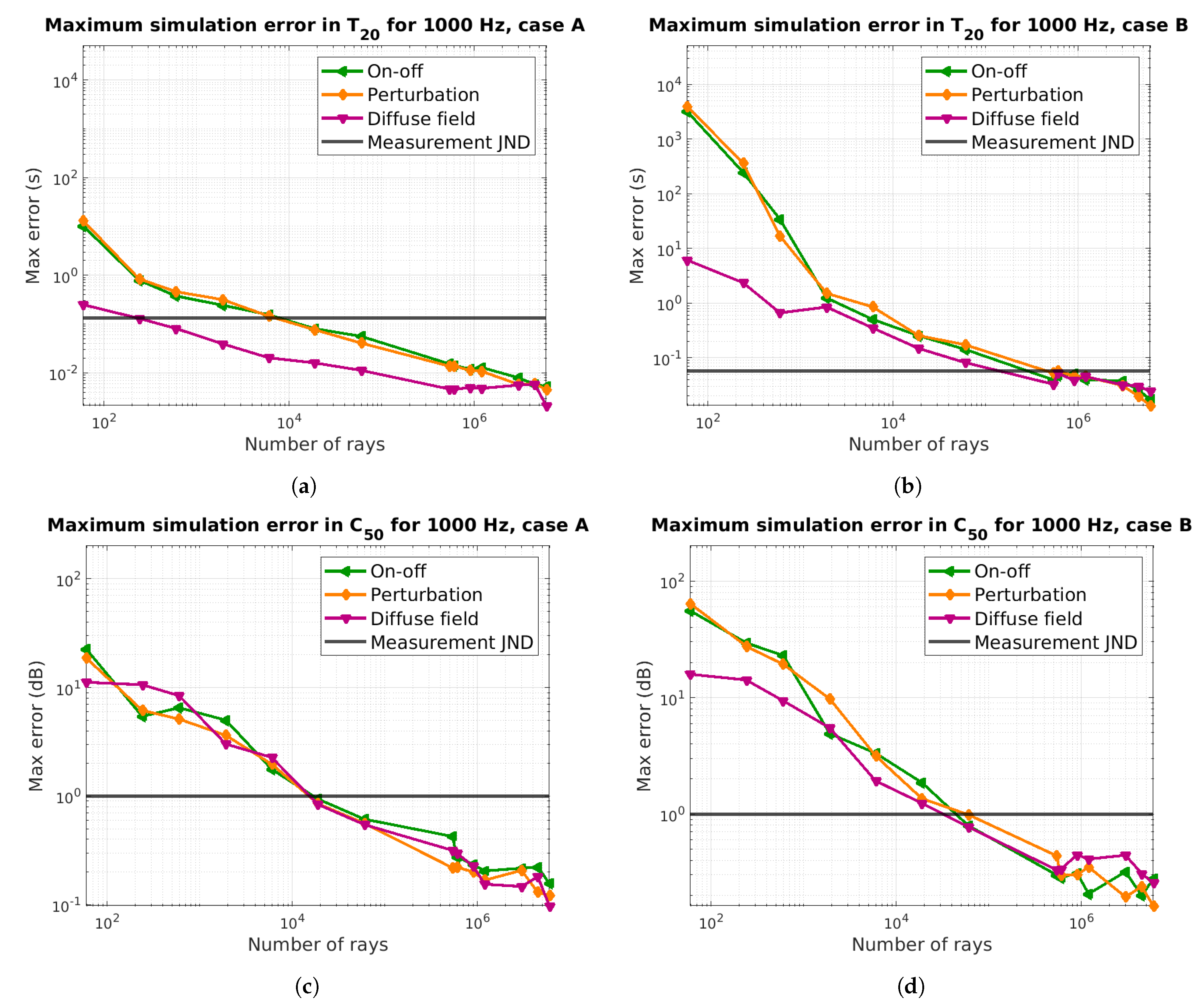
As a first step in measuring the time needed for a simulation of each algorithm, the number of rays needed is determined using the maximum simulation error $e_{\mathrm{Sim}}$, as defined in 2 in Section 3.2. The $e_{\mathrm{Sim}}$ calculated for $T_{20}$ and $C_{50}$ is shown in Figure 7. Since the results for the EDT are very similar to the results for $C_{50}$, they are not shown here. As expected, the error decreases as the number of rays increase. The number of rays needed for $e_{\mathrm{Sim}}$ to be below 1 JND is presented in

Table 4. The number of rays needed for the $e_{\mathrm{Sim}}$ to be below 1 JND for all the examined room acoustic parameters and the time consumption for such a simulation. More rays are needed for all algorithms in Case B.

	Algorithm	Number of Rays	Time Consumption (s)
Case A	On-off	60,000	1.23
	Perturbation	60,000	1.25
	Diffuse Field	60,000	1.98
Case B	On-off	540,000	2.80
	Perturbation	540,000	2.54
	Diffuse Field	540,000	2.84

. It should be noted again that $e_{\mathrm{Sim}}$ does not relate to physical accuracy, and the results here indicate whether the calculated response matches the underlying model, not whether it matches reality.

In Figure 7, it is shown that $e_{\mathrm{Sim}}$ for $T_{20}$ in case A is smaller for the diffuse field algorithm than the other two. This also occurs for small numbers of rays in case B. The reverberation time is related to the late, more reverberant parts of the sound field, which for the diffuse field algorithm corresponds to the parts of the sound field that are modeled using the diffuse field assumptions. The relatively small simulation error for $T_{20}$ shows that the methods for calculating the decay rate and energy added to the diffuse field are reliable and numerically stable in the chosen implementation.

From the results presented in Table 4, there are no significant differences in the number of rays needed for each of the algorithms. If only reverberation time was considered, it is likely that the diffuse field algorithm would outperform the others, based on the results in Figure 7.

It is also shown in Figure 7 that simulations in case B need more rays before $e_{\mathrm{Sim}}$ is small enough. Since theoretical estimates of the standard deviation of raytracing results indicate that the error should decrease as the equivalent absorption area increases [2], these results are somewhat unexpected. Although the standard deviation and the $e_{\mathrm{Sim}}$ are not identical, they should generally follow the same tendencies and it is thus expected that $e_{\mathrm{Sim}}$ should be smaller in case B. However, the theoretical estimate of the standard deviation requires the absorption to be relatively uniformly distributed in the test space, which is not the case for case B. Instead, the increased error $e_{\mathrm{Sim}}$ indicates that the complexity of the sound field has increased as the patch of high-absorption material was added.

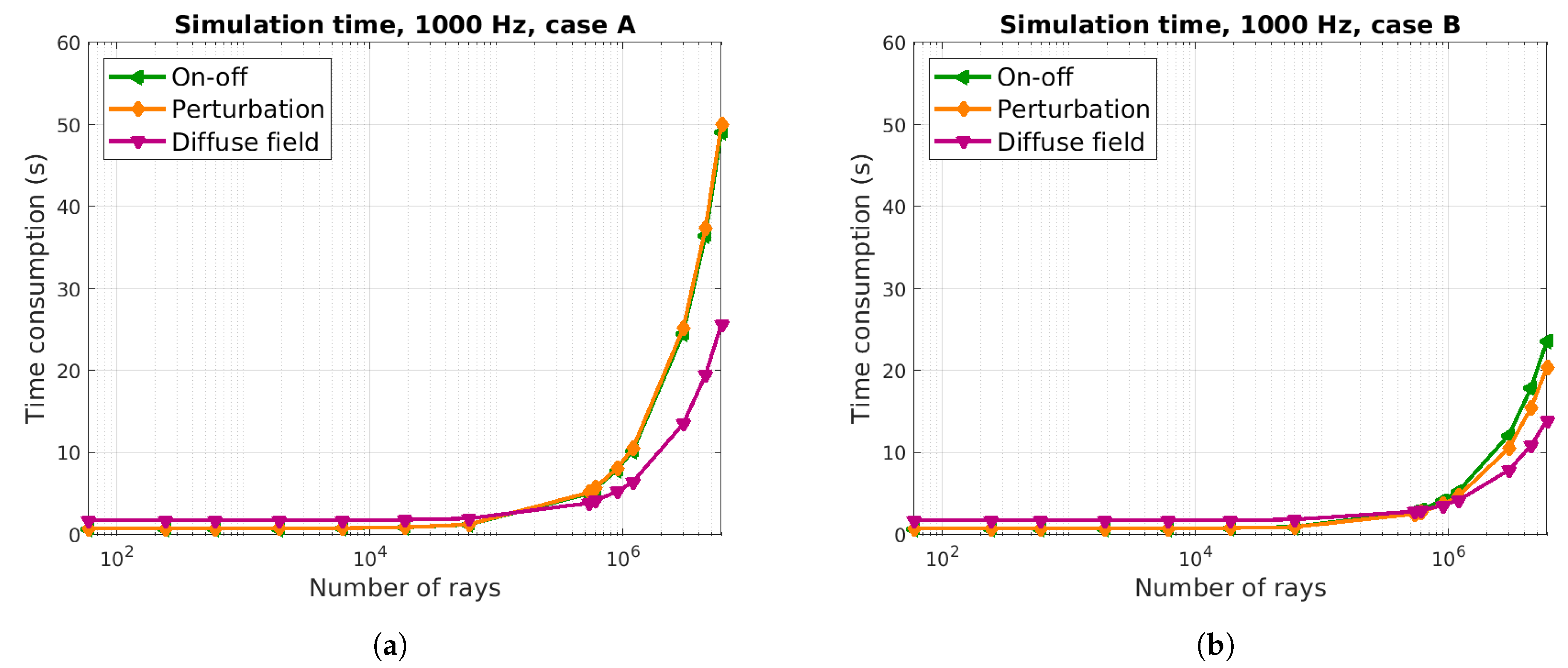
The time needed for running a raytracing simulation for a varying number of rays for each of the algorithms is shown in Figure 8. The time measured includes the raytracing for all four listener positions and one of the source positions for all frequency bands. The diffuse field algorithm data includes the raytracing step used to determine the diffuse field decay rate. The results presented in this graph are used together with the results shown in Figure 7 to estimate the time needed for a simulation, shown in Table 4.

Table 4 shows that the on–off and perturbation scattering algorithms have similar time consumption, while the diffuse field scattering algorithms is slower in case A and similar in case B.

Some more comments can be made regarding the results in Figure 8. Firstly, it is noted that for small numbers of rays, the time consumption does not increase substantially as the number of rays increases. This is because the NVIDIA OptiX raytracing engine used for these simulations is well-optimized, and many ray paths are traced simultaneously. Consequently, the time consumption does not increase until the number of rays exceed some threshold which seems to be at about 10,000 rays in this case. This value is consistent across all algorithms.

Secondly, it is noted that the overall simulation time for a given number of rays is smaller in case B than in case A. This is caused by the increased absorption in case B. Each individual ray is propagated until its energy falls below some threshold, and the primary mechanism for energy reduction is reflection in an absorptive surface. When more absorption is introduced, the rays decrease in energy more quickly and are thus terminated more quickly. Once all rays have been terminated, the trace is complete.

This effect is also a probable explanation for the shorter simulation time for high numbers of rays in the diffuse field algorithm. In the diffuse field scattering algorithm, the energy of each ray is reduced according to the scattering parameter in addition to the energy reduction introduced by the absorption parameter. Although this energy is accounted for in the diffuse field model, it leads to a faster termination of the rays nonetheless.

Although the diffuse field algorithm is faster for high numbers of rays, the same is not true for small numbers of rays. This is likely due to the additional computational overhead associated with the additional raytracing step for calculating the diffuse field decay rate. This is the reason for the longer overall simulation time seen for the diffuse field algorithm in case A in Table 4.

These results indicate some differences between the algorithms. In test spaces where a relatively low number of rays are needed, the on–off and perturbation algorithms are faster. However, when more rays are needed the diffuse field scattering algorithm outperforms the others in terms of speed.

5.3. Usability

Finally, the usability of the three algorithms is studied, primarily with regards to the effects of changes to the scattering parameters. In Figure 9, the effects on room acoustic parameters as the scattering value changes are shown for the octave band centered on 1000 Hz. In case B especially, increases to the scattering parameter lead to decreased reverberation as measured both by $T_{20}$ and EDT. It also leads to increased speech clarity $C_{50}$. The reduced reverberation is consistent with previous research in similar test spaces [10,13], while the previous results for speech clarity are inconclusive.

Changes to the ceiling absorbent scattering parameter do not affect the overall simulation outcome. This is explained by the high absorption coefficient of this surface. As shown in Table 1, the absorbent ceiling has an absorption coefficient of 0.95. Since scattering only acts on the energy which is reflected from a surface, even a scattering parameter of 1 can affect only 5% of the total incident energy on this surface. In this case, this seems to not be sufficient to have an impact on the simulated sound field. In the remainder of this section, only the scattering parameter for the remaining surfaces is considered.

From a technical perspective, the correlation between decreased reverberation and increased scattering in the on–off and perturbation scattering algorithms can be explained by considering the path of individual rays. If there is no scattering, a ray might remain bouncing between parallel walls for a long time. If these walls are relatively far apart, the energy of the ray decreases slowly. Towards the end of the simulation only these rays remain, and they thus dominate the late response. This can be seen in the simulation results as prolonged energy decay and consequently a long reverberation time. When on–off or perturbation scattering is introduced, the likelihood that a ray should be reflected away from that state increases and on average, each ray will be reflected between parallel walls for a shorter time. The overall reverberation is thus decreased.

In the diffuse field algorithm, the directions of individual rays are not affected by changes to the scattering parameter. Instead, increases to the diffuse field scattering parameter is directly interpreted as a transfer of energy (and thus an energy reduction) in each ray reflection in the traditional raytracing segment of the model. Therefore, the reverberation in this part of the model trivially decreases as the diffuse field scattering parameter increases. Furthermore, the energy transferred from the image source model in this way is added to the diffuse field, which has a decay rate corresponding to rays reflected in a random direction in each reflection. This matches simulations using the on–off scattering or perturbation algorithm with scattering parameters equal to the maximum value 1 and decay quickly, based on the argument in the previous paragraph. The reverberation found in the diffuse field scattering algorithm is thus doubly decreased by increases to the scattering parameter.

As seen in Figure 9, the changes to the sound field caused by changes in the scattering parameter are much more significant in case B than in case A. This is due to the difference in the distribution of absorption between the two cases. In case A, redirection of acoustic energy cannot cause it to immediately interact with a much more absorptive surface as none exist. However, in case B scattering effects will more often lead to reflection in a very absorptive surface and immediate energy reduction. Consequently, the effects of scattering in raytracers are much more pronounced in spaces with unevenly distributed absorption.

An aspect of usability is that the effects of changes to the scattering parameter should be predictable. The significant differences between case A and case B, and the two types of surface in case B, show that the effects of changes to the scattering parameters, to some extent, are unpredictable for all three algorithms. However, the perturbation algorithm is more unpredictable than either the on–off scattering algorithm or the diffuse field algorithm. In Figure 9, it is seen that all the room acoustic parameters may either increase or decrease as the perturbation scattering parameter increases. This makes the perturbation algorithm more difficult to use. In cases where the perturbation scattering parameter needs to be tuned, it may be difficult or impossible to determine whether it should be increased or decreased. Sometimes, both options may work and sometimes neither.

Another aspect of usability is whether small changes to the input parameter leads to small changes in the simulation output. As seen in Figure 9, the magnitude of the changes in simulated room acoustic parameters vary significantly depending on the space in question and the absolute value of the scattering parameter. In general, it seems that the effects of changing the scattering parameter is much smaller in spaces with more uniform absorption, which is an expected result. It also seems that modifications to the scattering parameters when it is fairly large has a relatively small impact on the simulated room acoustic parameters. These results replicate previous knowledge [10,13,28].

For the diffuse field algorithm in case B, the output variations are particularly large for small values in the scattering parameter (as shown in Figure 3 and Figure 4). In some cases, minimal changes might lead to changes more prominent than 1 JND in the simulated room acoustic parameters. This shows that the diffuse field algorithm in some cases is very sensitive to variations in the scattering parameter, which consequently must be provided to a very high level of accuracy. Since the diffuse field scattering parameter does not have a well-defined physical counterpart, it cannot be measured and is very difficult to estimate, making it more or less impossible to estimate to the required level of accuracy.

Finally, an aspect of usability is whether reasonable input values lead to reasonable output values. In Section 3.3, it is determined that a fair initial guess of the scattering parameters at mid-frequency would be $0.1$. A review of the results shown in Figure 9 shows that the results for this value are generally within a few JNDs for all algorithms in case A and the on–off and perturbation algorithms in case B. These results are not good but can be considered reasonable.

6. Discussion

Regarding physical accuracy, the diffuse field and perturbation algorithms perform worse than the on–off algorithm. However, their results show similar trends. They all show acceptable results for spatial averages in high frequencies, but cannot accurately model the sound field below 500 Hz, and do not emulate the spatial variations. The poor performance for low frequencies is consistent with the known limitations of raytracers [1,11], although it extends well above the Schröder frequency for the space in question. The discrepancies between measurements and simulations regarding spatial variations are somewhat unexpected. In any case, these issues are not useful to distinguish between the algorithms.

In general, the differences between the algorithms are seen much more clearly in the results for case B compared to case A. This suggests that surface scattering has a larger impact on the sound field in spaces with non-uniformly distributed absorption. Consequently, the choice of scattering algorithm and parameter requires extra care in spaces with localized absorption surfaces.

The diffuse field algorithm underperforms, as mentioned, in terms of physical accuracy in case B. The explanation presented in the analysis is that its underlying diffuse field model does not accurately describe a significant part of the acoustic field in case B. Since the model is inaccurate, the scattering algorithm based on it produces inaccurate simulation results. This explanation suggests that a more accurate physical model for the scattered energy can be developed and used as a foundation for a more accurate simulation algorithm, which still functions in a way similar to the diffuse field scattering algorithm. An example of such an extension is presented in [23], and it may also be possible to develop models based on acoustic radiosity or even Statistical energy analysis (SEA) similar to the model in [32]. The model must lend itself to fast and stable numerical calculations so that the benefits seen for the diffuse field algorithm in terms of time consumption are not lost.

The diffuse field scattering parameter and its effects on the simulation results are also affected by the inaccuracy of the diffuse field model in case B, negatively impacting the algorithm’s usability. The diffuse field simulation results are exceedingly sensitive to variations in the diffuse field scattering parameter, and the tuned parameter values are different from what was expected. As mentioned in Section 2, it was mentioned that the diffuse field scattering parameter can be interpreted as a weighting coefficient, determining the relative influence of the underlying image source and diffuse field models. With this interpretation, the small value of the diffuse field scattering parameter in case B indicates that the diffuse field model is more inaccurate in describing the sound field in the space as compared to the image source model. In addition, the high sensitivity in simulation outcome shows that there are large differences between the two models in this case.

One of the differences between the on-off and perturbation scattering algorithm is that the perturbation scattering algorithm is less predictable in terms of changes to its scattering parameter. It was noted that increases in the perturbation scattering parameter might lead to increases or decreases in reverberation time. This study has not investigated whether this may be physically accurate, but it has been identified as a significant issue for the usability of the perturbation scattering algorithm.

The tuned scattering parameters are different for the three algorithms, showing that it is difficult or impossible to define a single value that would work for all algorithms. It was noted already in Section 2 that the physical interpretation of the scattering parameter differs in the various algorithms. It is consequently not surprising to see that different values are appropriate. However, it underscores the fact that caution should be exercised when setting up the material properties in a simulation, as table values appropriate for one algorithm may not be appropriate for a different one. This emphasizes the role of the simulation engineer and their experience with the simulation software in achieving accurate simulation results. In future research, measured surface scattering coefficients as defined in ISO 17497-1 and ISO 17497-2 [17,18] could be tried as scattering parameters in various algorithms. Doing so would improve understanding of the connection between the physical phenomena of surface scattering and how it is measured and the algorithms’ scattering parameters.

This study has not indicated a significant difference between the three algorithms in terms of simulation time for the test space in question. The diffuse field algorithm seems able to reliably estimate the reverberation time in a simple space with relatively few rays, but this property does not extend to other room acoustic parameters. If many rays are used, the diffuse field algorithm is faster for the space examined in this study. It is unclear whether these results can be generalized. Notably, the diffuse field algorithm is prone to errors when the sound field deviates from the diffuse field approximation. Consequently, if a highly non-diffuse sound field causes the need for high numbers of rays, the diffuse field algorithm is inappropriate regardless of its fast calculation speed.

7. Conclusions

The goal of this study is to evaluate the influence of the scattering algorithm in acoustic raytracers. To this end, three algorithms are compared: The on–off scattering algorithm, the perturbation scattering algorithm and the diffuse field scattering algorithm. It is found that the choice of scattering algorithm impacts raytracers’ physical accuracy, simulation speed, and usability. In addition, the scattering parameter must be chosen based on the scattering algorithm used.

Out of the on–off, perturbation and diffuse field scattering algorithms, the on–off scattering algorithm is most appropriate for raytracers based on its better usability and physical accuracy. A more complex test space with directional scatterers may yield further insights into the on–off scattering algorithm’s strengths and weaknesses.