
Hysteresis Envelope Model of Double Extended End-Plate Bolted Beam-to-Column Joint


Abstract
1. Introduction
2. Numerical Model of Joint
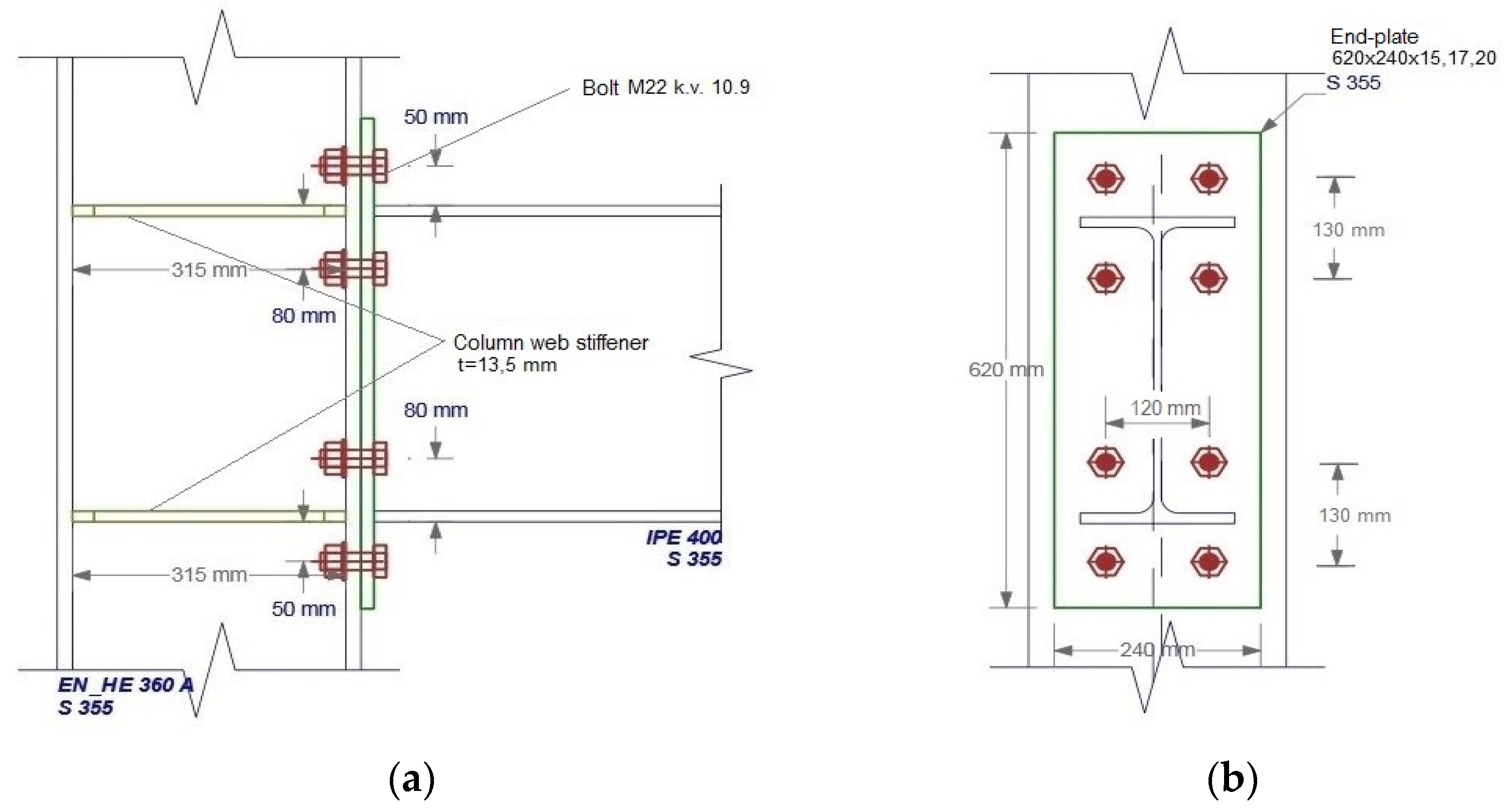
2.1. Geometry of Joints
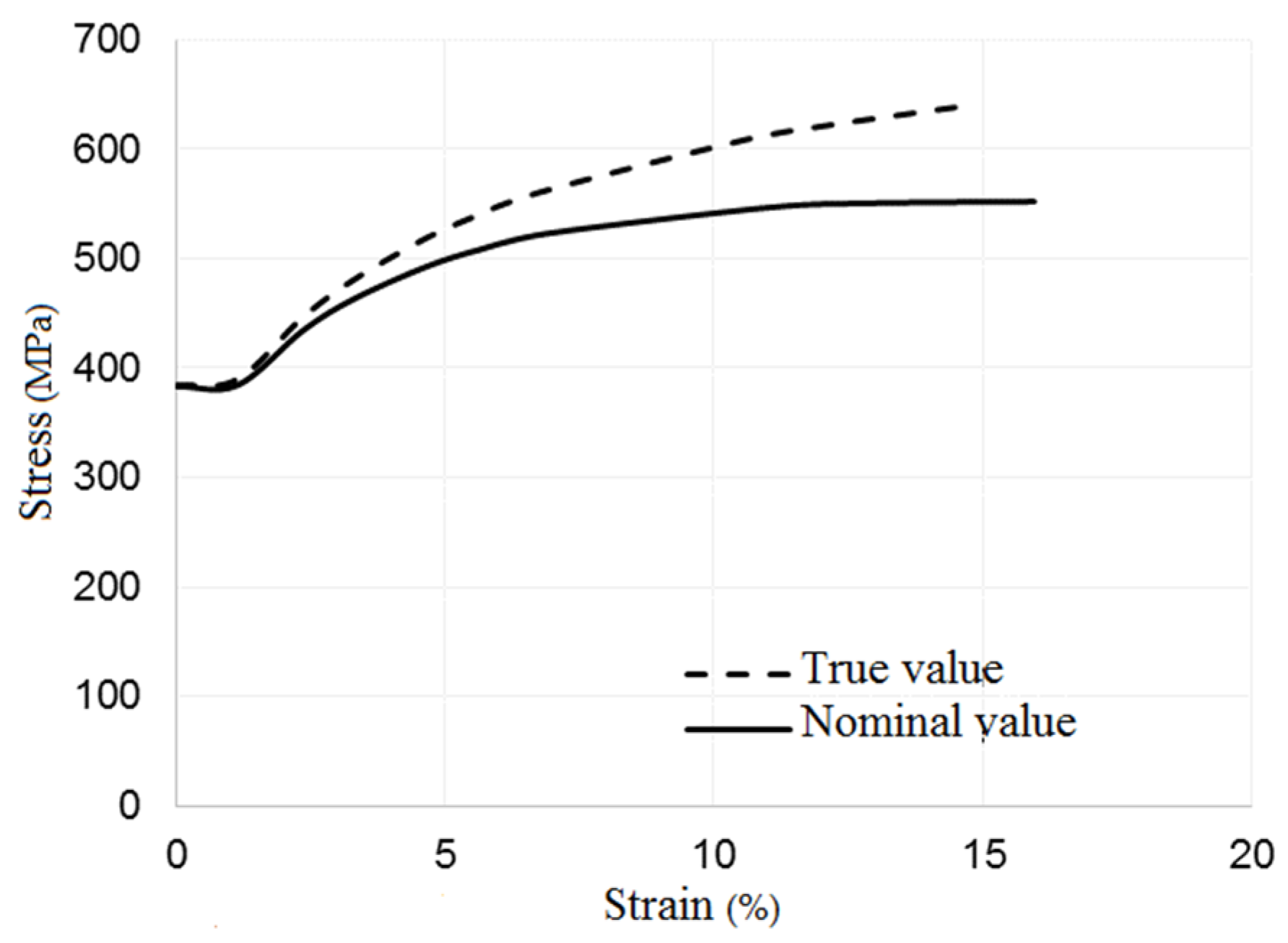
2.2. Material Properties
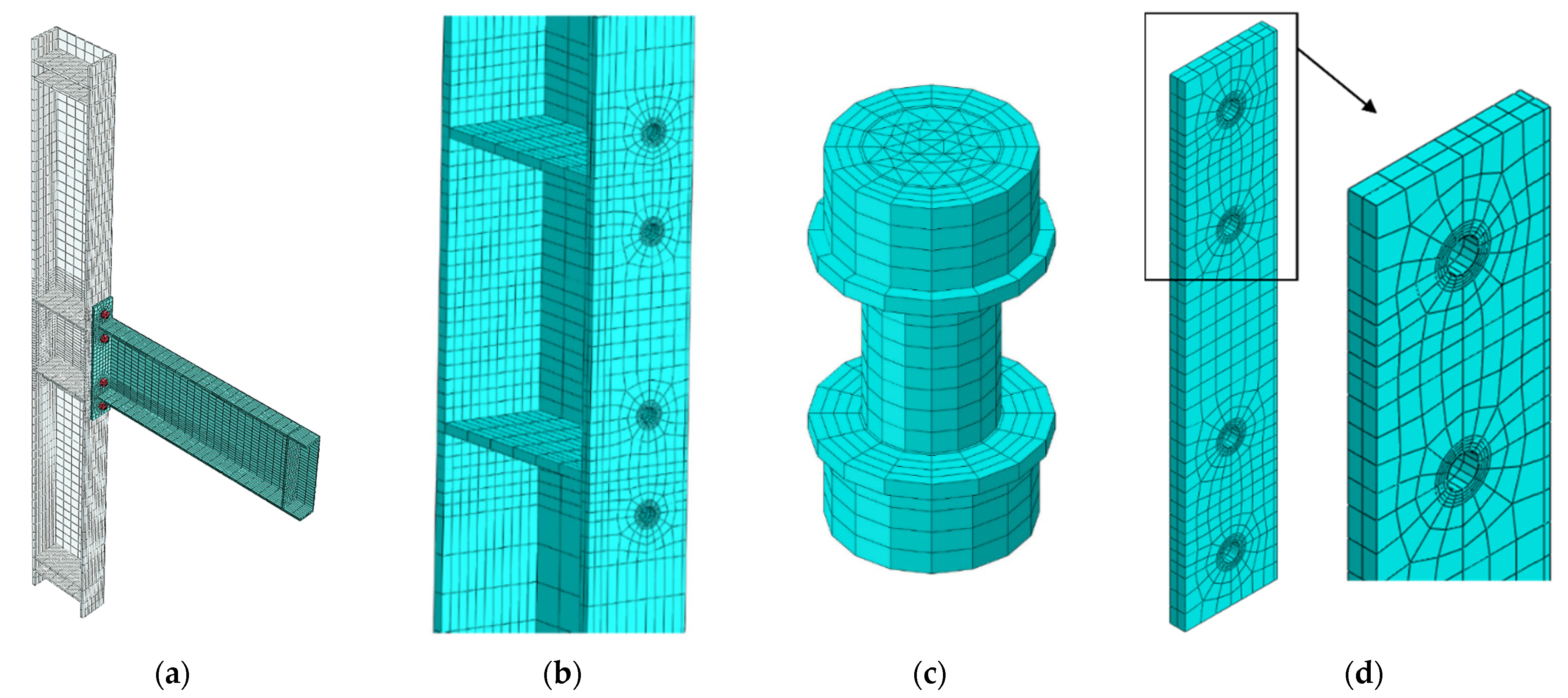
2.3. Finite Element Mesh
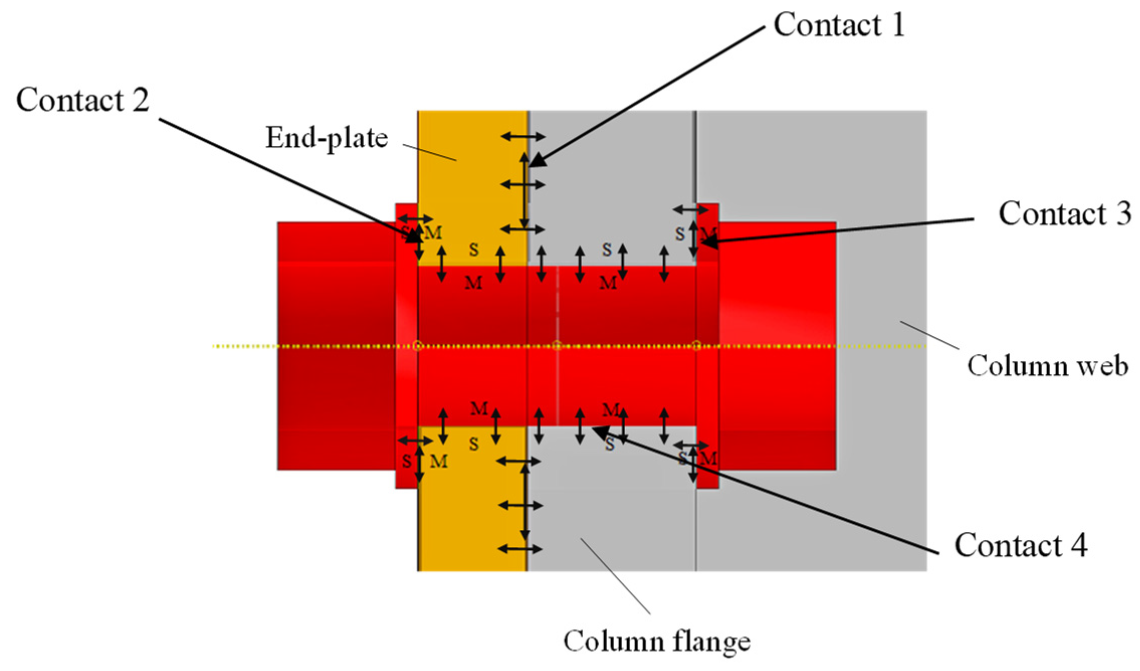
2.4. Contact Modelling
2.5. Bolt Pretension
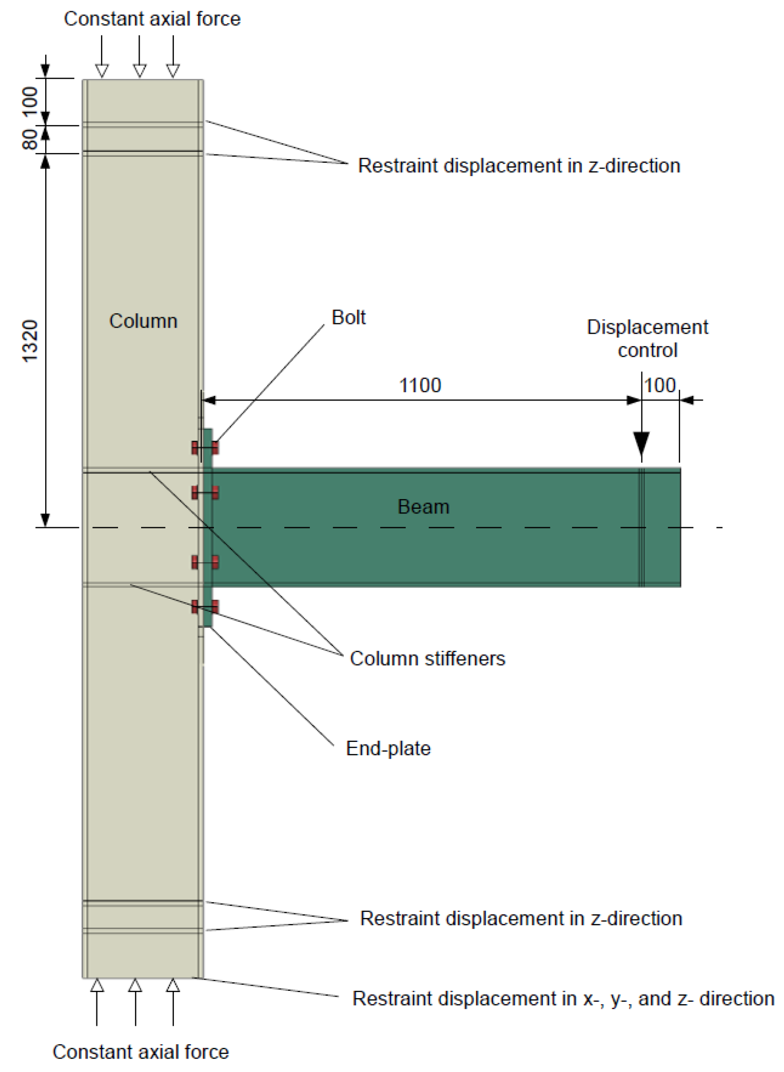
2.6. Boundary Condition and Loading Procedure
2.7. Results of Numerical Simulation
2.8. Calibration of Numerical Model
3. Mathematical Model of Hysteresis Envelope
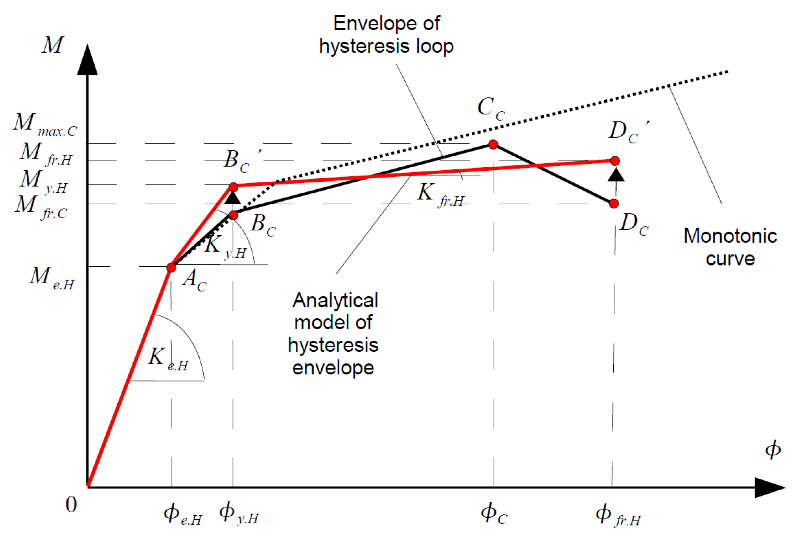
3.1. Proposal of Hysteresis Envelope Model
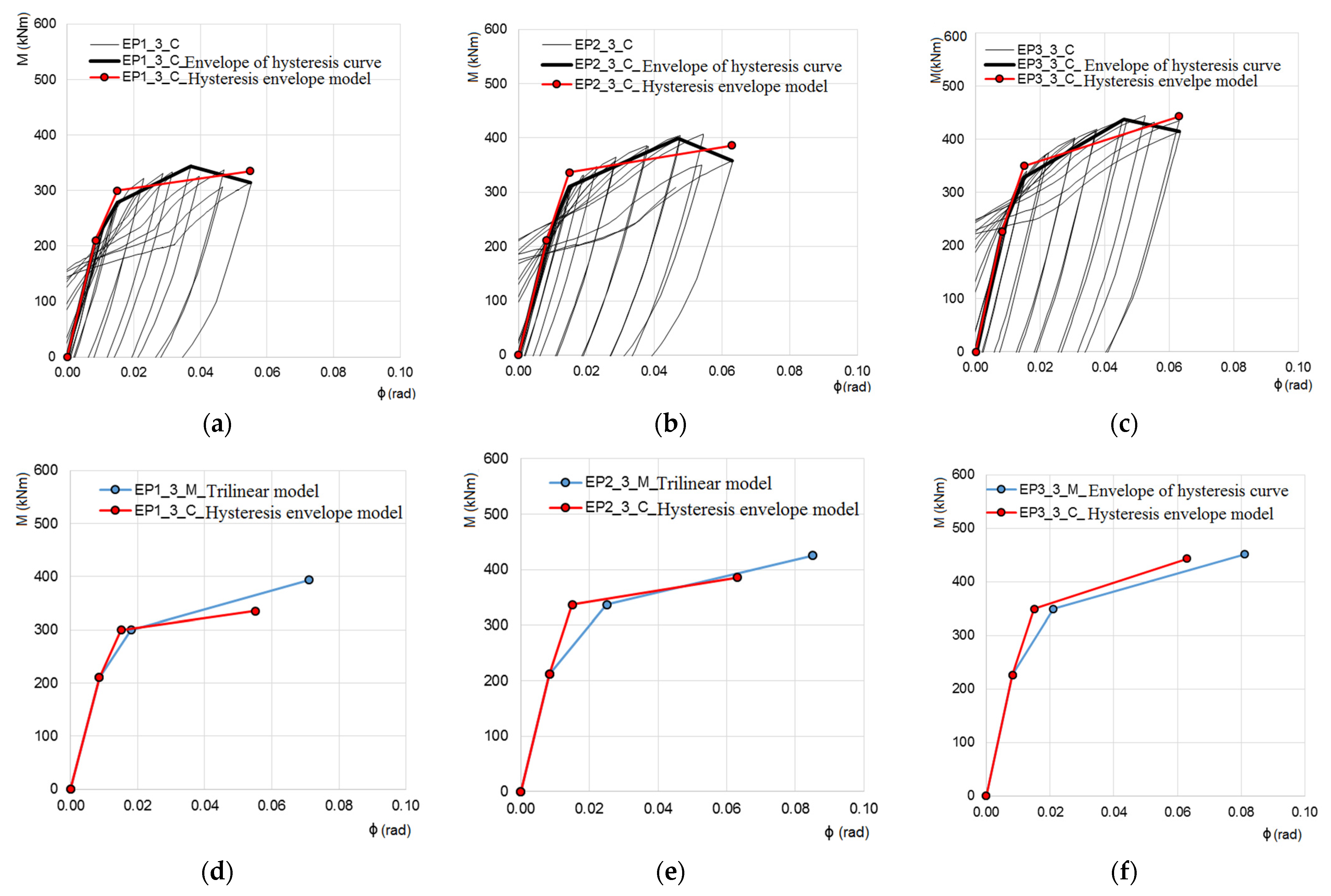
3.2. Regression Analysis
4. Seismic Analysis
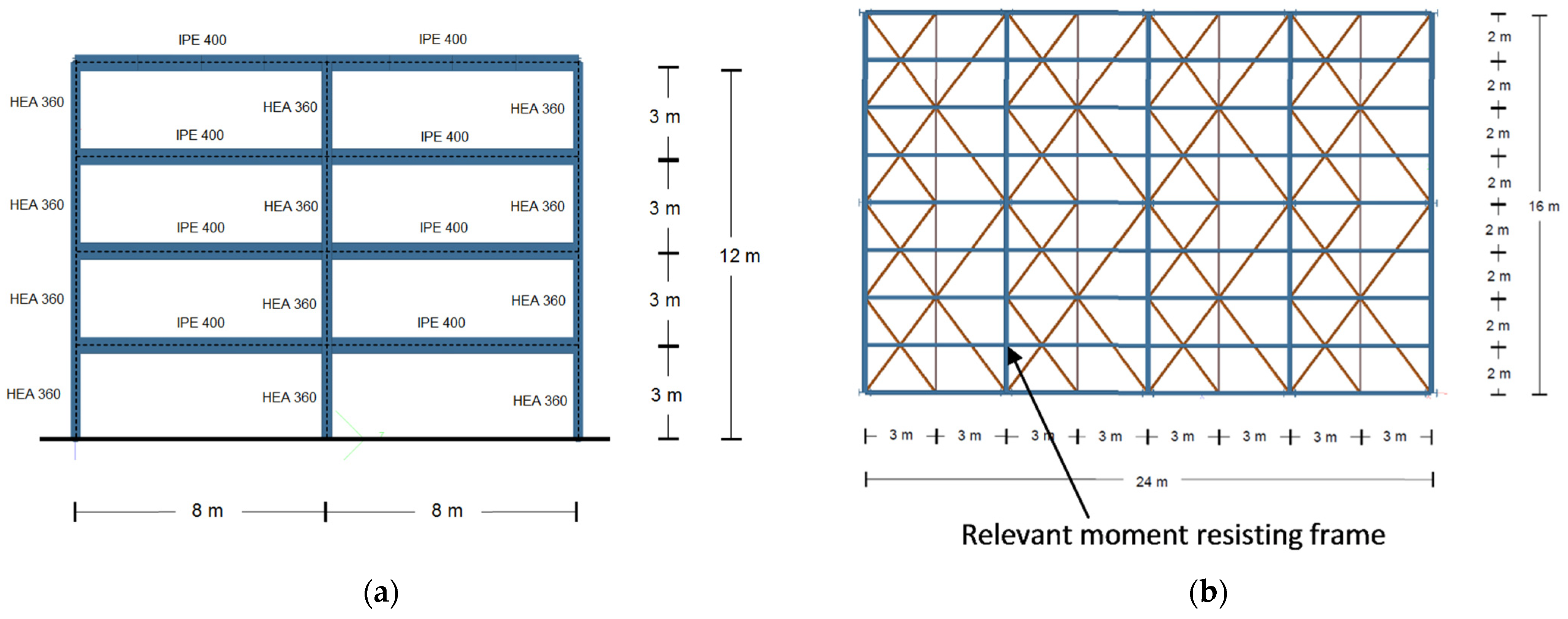
4.1. Description of the Building
4.2. Trilinear Joint Model
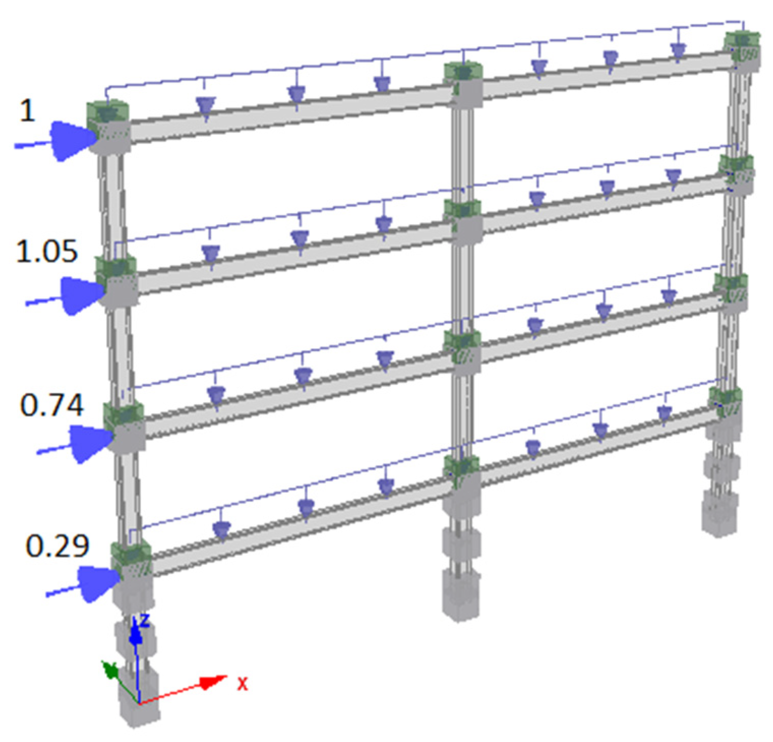
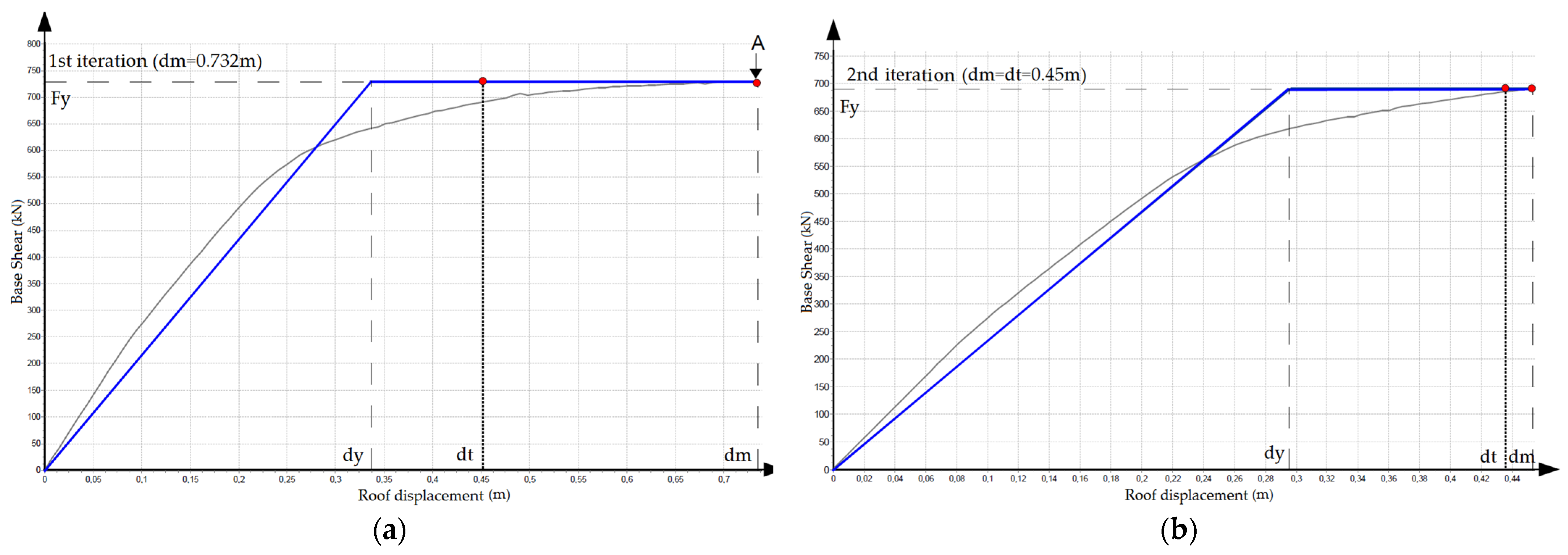
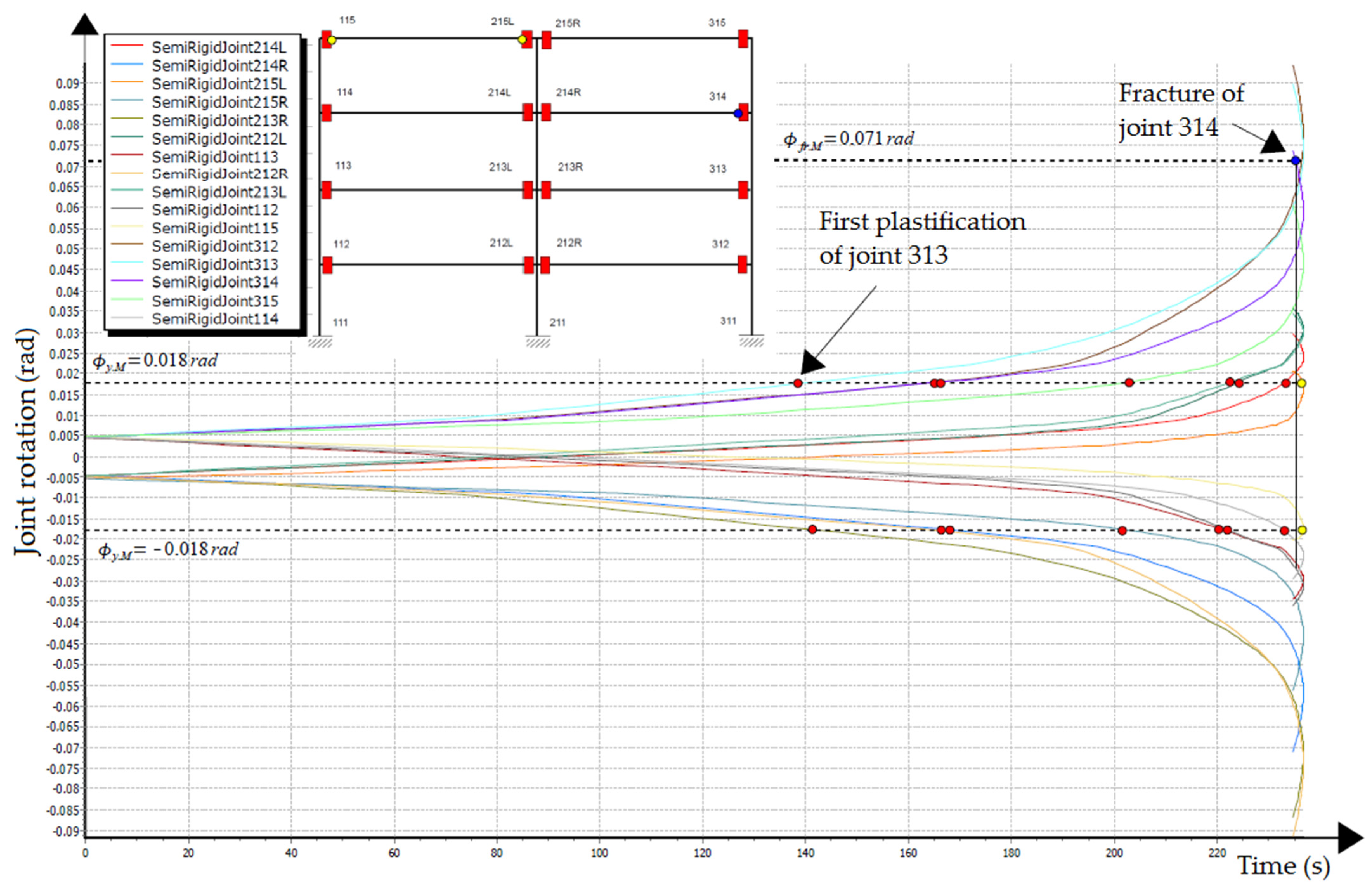
4.3. Nonlinear Static Pushover Analysis (N2 Method)
5. Conclusions
Author Contributions
Funding
Institutional Review Board Statement
Informed Consent Statement
Data Availability Statement
Conflicts of Interest
References
- Adey, B.T.; Grondin, G.Y.; Cheng, J.R. Cyclic loading of end plate moment connections. Can. J. Civ. Eng. 2000, 27, 683–701. [Google Scholar] [CrossRef]
- Gioncu, V.; Mazzolani, F.M. Ductility of Seismic Resistant Steel Structures; Spon Press: London, UK, 2002. [Google Scholar]
- Mazzolani, F.M.; Piluso, V. Theory and Design of Seismic Resistant Steel Frames; E&FN Spon: London, UK, 1996. [Google Scholar]
- Abolmaali, A.; Kukreti, A.R.; Motahari, A.; Ghassemieh, M. Energy disspation characteristics of semi-rigid connection. J. Constr. Steel Res. 2009, 65, 1187–1197. [Google Scholar] [CrossRef]
- Kukreti, A.R.; Abolmaali, A. Moment rotation hysteresis behaviour of top and seat angle steel frame connections. J. Struct. Eng. 1999, 125, 810–820. [Google Scholar] [CrossRef]
- Abolmaali, A.; Matthys, J.H.; Farooqi, M.; Choi, Y. Development of moment-rotation model equations for flush end plate connections. J. Constr. Steel Res. 2005, 61, 1595–1612. [Google Scholar] [CrossRef]
- Shi, G.; Shi, Y.; Wang, Y. Behaviour of end-plate moment connections under earthquake loading. Eng. Struct. 2007, 29, 703–716. [Google Scholar] [CrossRef]
- Fajfar, P. A Nonlinear Analysis Method for Performance Based Seismic Design. Earthq. Spectra 2000, 16, 573–592. [Google Scholar] [CrossRef]
- Nogueiro, P.; Bento, R.; da Silva, L.S. Evaluation of the ductility demand in partial strength steel structures in seimsic areas using non-linear static analysis. In Progress in Steel, Composite and Aluminium Structures: Proceedings of the XI Int Conf on Metal Structures, Rzeszow, Poland, 21–23 June 2006; CRC Press: Rzeszow, Poland, 2006; pp. 268–278. [Google Scholar]
- Krolo, P.; Čaušević, M.; Bulić, M. Seismic analysis of framed steel structure with semi-rigid joints. In Proceedings of the 7th European Conference on Steel and Composite Structures, Naples, Italy, 10–12 September 2014; Landolfo, R., Mazzolani, F.M., Eds.; ECCS: Napoli, Italy, 2014; pp. 1–6. [Google Scholar]
- Krolo, P.; Čaušević, M.; Bulić, M. Nonlinear seismic analysis of steel frame with semi-rigid joints. Građevinar 2015, 67, 573–583. [Google Scholar] [CrossRef][Green Version]
- Krolo, P.; Čaušević, M.; Bulić, M. The extended N2 method in seismic design of frames considering semi-rigid joints. In Proceedings of the 2th European Conference on Earthquake Engineering and Seismology, Istanbul, Turkey, 25–29 August 2014; Ansal, A., Ed.; Paper 302. European Association of Earthquake, Engineering (EAEE): Istanbul, Turkey, 2014; pp. 74–84. [Google Scholar]
- Ramberg, W.; Osgood, W.R. Description of stress-strain curves by three-parameters. In National Advisory for Aeronautics; Technical Report 902; 1943; Available online: http://www.apesolutions.com/spd/public/NACA-TN902.pdf (accessed on 31 October 2021).
- Ang, K.M.; Morris, G.A. Analysis of three-dimensional frames with flexible beam-column connections. Can. J. Civ. Eng. 1983, 11, 245–254. [Google Scholar] [CrossRef]
- Richard, R.M.; Abbott, B.J. Versatile elasto-plastic stress-strain formula. J. Eng. Mech. 1975, 101, 511–515. [Google Scholar]
- Attiogbe, G.; Morris, G. Moment-rotation functions for steel connections. J. Struct. Eng. 1991, 117, 1703–1718. [Google Scholar] [CrossRef]
- Krishnamurthy, N.; Graddy, D.E. Correlation between 2- and 3-dimensional finite element analysis of steel bolted end-plate connections. Comput. Struct. 1976, 6, 381–389. [Google Scholar] [CrossRef]
- Yee, Y.; Melchers, R. Momenr-Rotation Curve for Bolted Connections. J. Struct. Eng. 1986, 112, 615–635. [Google Scholar] [CrossRef]
- Wu, F.H.; Chen, W.F. A design model for semi-rigid connections. Eng. Struct. 1990, 12, 88–97. [Google Scholar] [CrossRef]
- De Martino, A.; Faella, C.; Mazzolani, F.M. Simulation of Beam-to-Column Joint Behaviour under Cyclic Loads. Construzioni Met. 1984, 6, 346–356. [Google Scholar]
- Della Corte, G.; De Matteis, G.; Landolfo, R. Influence of Connection Modelling on Seismic Response of Moment Resisting Steel Frames. In Moment Resistant Connections of Steel Buildings Frames in Seismic Areas; E.&F.N. Spon: London, UK, 2000. [Google Scholar]
- Nogueiro, P.; da Silva, L.S.; Bento, R. Influence of joint slippage on the cyclic response of steel frames. In Proceedings of the 9th International Conference on Civil and Structural Engineering Computing, Egmond-aan-Zee, The Netherlands, 2–4 September 2003; Civil-Comp Press: Egmond-aan-Zee, The Netherlands, 2003. [Google Scholar]
- Lignos, D.G.; Krawinkler, H. Deterioration modeling of steel components in support of collapse prediction of steel moment frames under earthquake loading. J. Struct. Eng. 2011, 137, 1291–1302. [Google Scholar] [CrossRef]
- Elkady, A.; Lignos, D.G. Analytical investigation of the cyclic behavior and plastic hinge formation in deep wide-flange steel beam-columns. Bull. Earthq. Eng. 2015, 13, 1097–1118. [Google Scholar] [CrossRef]
- Cravero, J.; Elkady, A.; Lignos, D.G. Experimental evaluation and numerical modeling od wide-flange steel columns subjected to constant and variable axial load coupled with lateral drift demands. J. Struct. Eng. 2020, 146, 04019222. [Google Scholar] [CrossRef]
- PEER and ATC (Pacific Earthquake Engineering Research Center and Applied Technology Council). Modelling and Acceptance Criteria for Seismic Design and Analysis of Tall Building PEER/ATC 71-1; PEER and ATC: Redwood City, CA, USA, 2010. [Google Scholar]
- EN1993-1-8:2014. Eurocode 3: Design of Steel Structures—Part 1–8: Design of Joints (EN 1993-1-8:2005+AC:2009). Available online: https://www.phd.eng.br/wp-content/uploads/2015/12/en.1993.1.8.2005-1.pdf (accessed on 15 September 2021).
- ABAQUS. Analysis User’s Manual I_V, Version 6.12; Dassault Systemes: Fremont, CA, USA, 2012. [Google Scholar]
- Shi, G.; Shi, Y.; Wang, Y.; Bijlaard, F. Monotonic Loading Tests on Semi-Rigid End-Plate Connections with Welded I-Shaped Columns and Beams. Adv. Struct. Eng. 2010, 13, 215–229. [Google Scholar] [CrossRef]
- Krolo, P.; Grandić, D.; Bulić, M. The guidelines for modeling the preloading bolts in the structural connection using finite element method. J. Comput. Eng. 2016, 2016, 4724312. [Google Scholar] [CrossRef]
- Rice, J.; Tracey, D. On the Ductile Enlargement of Voids in Triaxial Stress Fields. J. Mech. Phys. Solids 1969, 17, 201–217. [Google Scholar] [CrossRef]
- Krolo, P. Influence of Bolted Joints Behaviour on Seismic Response of Steel Frames. Ph.D. Thesis, Faculty of Civil Engineering University in Rijeka, Rijeka, Croatia, 2017. [Google Scholar]
- Wang, M.; Shi, Y.; Wang, Y.; Shi, G. Numerical study on seismic behaviors of steel frame. J. Constr. Steel Res. 2013, 90, 140–152. [Google Scholar] [CrossRef]
- SAC-SteelProject. Protocol for Fabrication, Inspection, Testing and Documentation of Beam-Column Connection Tests and Other Experimental Specimens; FEMA: Washington, DC, USA, 1997. [Google Scholar]
- Krolo, P.; Grandić, D.; Smolčić, Ž. Experimental and Numerical Study of Mild Steel Behaviour under Cyclic Loading with Variable Strain Ranges. Adv. Mater. Sci. Eng. 2016, 2016, 7863010. [Google Scholar] [CrossRef]
- EN-1998-1. Eurocode 8: Design of Structures for Earthquake Resistance—Part 1: General Rules, Seismic Actions and Rules for Buildings; European Committee for Standardization (CEN): Brussels, Belgium, 2004. [Google Scholar]
- SeismoSoft2020. SeismoStruct 2020—A Computer Program for Static and Dynamic Nonlinear Analysis of Framed Structures. Available online: https://seismosoft.com/ (accessed on 19 February 2020).
- Wang, T.; Wang, Z.; Wang, J.; Feng, J. A Simplified Calculation Model for Moment-rotation Curve Used in Semi-rigid End-plate Connections. J. Inf. Comput. Sci. 2013, 10, 3529–3538. [Google Scholar] [CrossRef]


| Group of Joints | FE Model | End-Plate Thickness (mm) | Bolts Row Spacing (mm) |
|---|---|---|---|
| EP1_1_M/EP1_1_C | 15 | 130 | |
| 1 | EP1_2_M/EP1_2_C | 140 | |
| EP1_3_M/EP1_3_C | 150 | ||
| EP2_1_M/EP2_1_C | 17 | 130 | |
| 2 | EP2_2_M/EP2_2_C | 140 | |
| EP2_3_M/EP2_3_C | 150 | ||
| EP3_1_M/EP3_1_C | 20 | 130 | |
| 3 | EP3_2_M/EP3_2_C | 140 | |
| EP3_3_M/EP3_3_C | 150 |
| Element/Cross Section | Height h (mm) | Width b (mm) | Flange Thickness tf (mm) | Web Thickness tw (mm) |
|---|---|---|---|---|
| Beam/IPE400 | 400 | 180 | 13.5 | 8.6 |
| Column/HEA360 | 350 | 300 | 17.5 | 10 |
| Damage Initiation Criteria | Damage Evaluation Low | |||
|---|---|---|---|---|
| D | ||||
| 0.2270 | 0.32 | 0.001 | 0 | 0 |
| 0.2070 | 0.50 | 0.001 | 0.0105 | 0.0580 |
| 0.1945 | 0.60 | 0.001 | 0.0305 | 0.0965 |
| 0.1822 | 0.70 | 0.001 | 0.0625 | 0.1346 |
| 0.1755 | 0.76 | 0.001 | 0.0872 | 0.1562 |
| 0.1676 | 0.82 | 0.001 | 0.1183 | 0.1788 |
| 0.1562 | 0.90 | 0.001 | 0.1701 | 0.2087 |
| 0.1502 | 0.95 | 0.001 | 0.2147 | 0.2295 |
| 0.1480 | 0.97 | 0.001 | 0.2304 | 0.2355 |
| Elastic Behaviour | Plastic Behaviour | |||||||||
|---|---|---|---|---|---|---|---|---|---|---|
| Kinematic Hardening | Isotropic Hardening | |||||||||
(MPa) | ||||||||||
| 185,000 | 0.3 | 386 | 5327 | 75 | 1725 | 16 | 1120 | 10 | 20.8 | 3.2 |
| Damage Initiation Criteria | Damage Evaluation Low | |||
|---|---|---|---|---|
| D | ||||
| 0.63080 | 0.33 | 0.001 | 0.0037 | 0.0000 |
| 0.62491 | 0.38 | 0.001 | 0.0085 | 0.4719 |
| 0.61874 | 0.43 | 0.001 | 0.0243 | 0.9666 |
| 0.61244 | 0.48 | 0.001 | 0.0623 | 1.4716 |
| 0.60607 | 0.52 | 0.001 | 0.1293 | 1.9823 |
| 0.59963 | 0.57 | 0.001 | 0.2386 | 2.4987 |
| 0.59310 | 0.61 | 0.001 | 1.0000 | 3.0220 |
| Stress | 990 | 1160 | 1160 |
| Strain | 0.00483 | 0.136 | 0.05 |
| Step | (rad) | Vertical Displacement at the End of the Beam (mm) | |
|---|---|---|---|
| 1 | 0.00375 | 6 | 3.28 |
| 2 | 0.005 | 6 | 4.38 |
| 3 | 0.0075 | 6 | 6.56 |
| 4 | 0.01 | 4 | 8.75 |
| 5 | 0.015 | 2 | 13.13 |
| 6 | 0.02 | 2 | 17.5 |
| 7 | 0.03 | 2 | 26.25 |
| 8 | 0.04 | 2 | 35.0 |
| 9 | 0.05 | 2 | 43.75 |
| 10 | 0.06 | 2 | 52.5 |
| 11 | 0.07 | 2 | 61.25 |
| 12 | 0.08 | 2 | 70 |
| Group of Joint | FE Model | ||||||
|---|---|---|---|---|---|---|---|
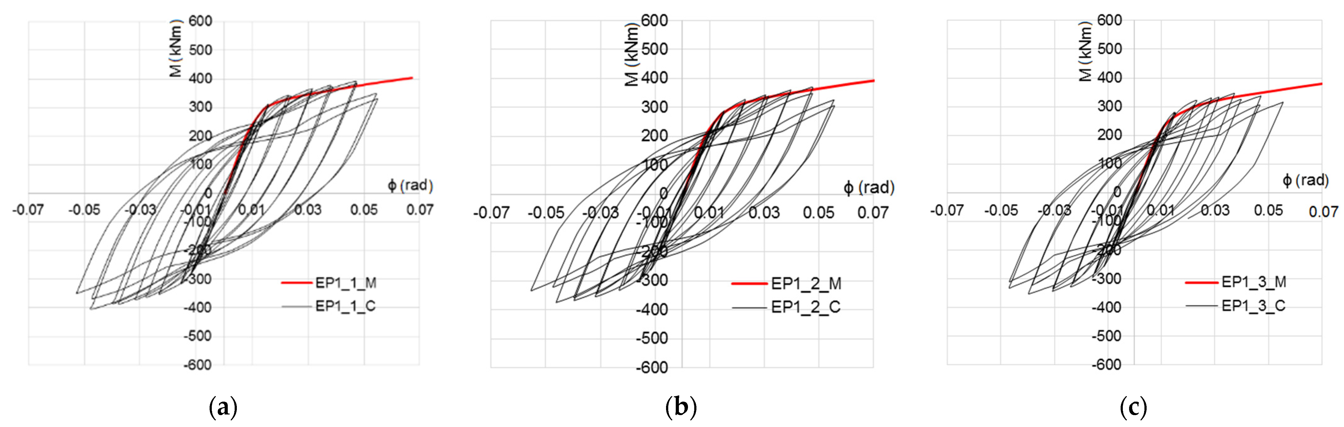
| 1 | EP1_1_M | 227.72 | 0.009 | 333.01 | 0.023 | 428.55 | 0.083 |
| EP1_2_M | 210.2 | 0.0085 | 307.63 | 0.021 | 401.82 | 0.078 | |
| EP1_3_M | 194.44 | 0.008 | 300.19 | 0.018 | 394.08 | 0.071 | |
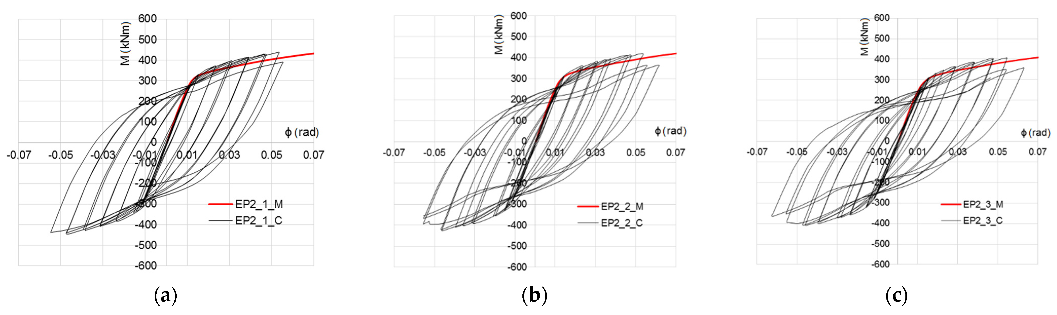
| 2 | EP2_1_M | 237.73 | 0.009 | 355.29 | 0.025 | 449.28 | 0.085 |
| EP2_2_M | 220.38 | 0.0085 | 340.11 | 0.023 | 430.87 | 0.079 | |
| EP2_3_M | 211.88 | 0.0083 | 331.05 | 0.023 | 415.02 | 0.075 | |
| 3 | EP3_1_M | 257.26 | 0.009 | 370.67 | 0.024 | 474.47 | 0.084 |
| EP3_2_M | 237.21 | 0.0085 | 359.2 | 0.023 | 460.04 | 0.081 | |
| EP3_3_M | 226.5 | 0.0082 | 349.68 | 0.021 | 451.38 | 0.081 |
| Group of Joint | FE Model | ||||||||
|---|---|---|---|---|---|---|---|---|---|
| 1 | EP1_1_C | 227.72 | 0.009 | 310.98 | 0.016 | 392.44 | 0.047 | 331.34 | 0.055 |
| EP1_2_C | 210.2 | 0.0085 | 287.99 | 0.0152 | 369.52 | 0.047 | 306.08 | 0.055 | |
| EP1_3_C | 194.44 | 0.008 | 278.89 | 0.0135 | 344.26 | 0.037 | 344.26 | 0.055 | |
| 2 | EP2_1_C | 237.73 | 0.009 | 330.02 | 0.0152 | 429.20 | 0.048 | 391 | 0.055 |
| EP2_2_C | 220.38 | 0.0085 | 313.88 | 0.0148 | 413.03 | 0.047 | 364.69 | 0.062 | |
| EP2_3_C | 211.88 | 0.0083 | 310.17 | 0.0143 | 399.65 | 0.047 | 358.16 | 0.063 | |
| 3 | EP3_1_C | 257.26 | 0.009 | 354.13 | 0.0157 | 461.86 | 0.046 | 451.09 | 0.063 |
| EP3_2_C | 237.21 | 0.0085 | 342.88 | 0.015 | 433.93 | 0.039 | 424.73 | 0.063 | |
| EP3_3_C | 226.5 | 0.0082 | 328.33 | 0.015 | 437.07 | 0.046 | 414.66 | 0.063 |
| Group of Joint | FE Model | ||||||
|---|---|---|---|---|---|---|---|
| 1 | EP1_1_M/EP1_1_C | - | - | 7.1 | 43.8 | 9.2 | 50.9 |
| EP1_2_M/EP1_2_C | - | - | 6.8 | 38.2 | 8.7 | 41.8 | |
| EP1_3_M/EP1_3_C | - | - | 7.6 | 33.3 | 14.5 | 29.1 | |
| 2 | EP2_1_M/EP2_1_C | - | - | 7.7 | 64.5 | 4.7 | 54.5 |
| EP2_2_M/EP2_2_C | - | - | 8.4 | 55.4 | 4.3 | 27.4 | |
| EP2_3_M/EP2_3_C | - | - | 6.7 | 60.8 | 3.8 | 19.0 | |
| 3 | EP3_1_M/EP3_1_C | - | - | 4.7 | 52.9 | 2.7 | 33.3 |
| EP3_2_M/EP3_2_C | - | - | 4.8 | 53.3 | 6.0 | 28.6 | |
| EP3_3_M/EP3_3_C | - | - | 6.5 | 40.0 | 3.3 | 28.6 | |
| | |||||||
| Kinematic Hardening | Isotropic Hardening | |||||||||
|---|---|---|---|---|---|---|---|---|---|---|
| 363.3 | 7993 | 175 | 6773 | 116 | 2854 | 34 | 1450 | 29 | 21 | 1.2 |
| Load Type | Numerical Simulations | Laboratory Test by Shi et al. [7,29] | ||
|---|---|---|---|---|
| Loading Capacity (kN) | Moment Resistance (kNm) | Loading Capacity (kN) | Moment Resistance (kNm) | |
| Monotonic | 256.89 | 308.28 | 256.9 | 308.3 |
| Cyclic | 237.89 | 285.47 | 251.9 | 288.4 |
| Group of Joint | Model | |||||
|---|---|---|---|---|---|---|
| 1 | EP1_1_C_ Hysteresis envelope model | 25,302.2 | 333.01 | 0.016 | 370.9 | 0.055 |
| EP1_2_C_ Hysteresis envelope model | 24,729.4 | 307.63 | 0.0152 | 351.5 | 0.055 | |
| EP1_3_C_ Hysteresis envelope model | 24,305 | 300.19 | 0.0135 | 335.8 | 0.055 | |
| 2 | EP2_1_C_ Hysteresis envelope model | 26,414.4 | 355.29 | 0.0152 | 411.0 | 0.055 |
| EP2_2_C_ Hysteresis envelope model | 25,927.1 | 340.11 | 0.0148 | 407.11 | 0.0615 | |
| EP2_3_C_ Hysteresis envelope model | 25,527.7 | 336.05 | 0.0143 | 392 | 0.063 | |
| 3 | EP3_1_C_ Hysteresis envelope model | 28,584.4 | 370.67 | 0.0157 | 477.9 | 0.063 |
| EP3_2_C_ Hysteresis envelope model | 27,907.1 | 359.2 | 0.015 | 456.1 | 0.063 | |
| EP3_3_C_ Hysteresis envelope model | 27,622.0 | 349.68 | 0.015 | 443.5 | 0.063 |
| Joint Model | |||
|---|---|---|---|
| EP1_3_M_Trilinear model | 24,305 | 0.435 | 0.073 |
| EP2_3_M_Trilinear model | 25,527.7 | 0.318 | 0.063 |
| EP3_3_M_Trilinear model | 27,622 | 0.348 | 0.061 |
| Model | Max | |||||||||
|---|---|---|---|---|---|---|---|---|---|---|
| Frame1_M | 0.73 | 511.71 | 0.219 | 1.65 | 0.33 | 0.49 | 31.18 | 1.51 | 43.44 | 0.51 |
| Frame1_C | 0.542 | 492.9 | 0.207 | 1.63 | 0.31 | 0.49 | 31.97 | 1.59 | 43.16 | 0.38 |
| Frame2_M | 0.893 | 526.33 | 0.224 | 1.64 | 0.33 | 0.49 | 32.14 | 1.48 | 43.39 | 0.62 |
| Frame2_C | 0.632 | 532.16 | 0.207 | 1.57 | 0.34 | 0.52 | 30.74 | 1.53 | 41.50 | 0.46 |
| Frame3_M | 0.853 | 539.48 | 0.213 | 1.58 | 0.34 | 0.51 | 31 | 1.49 | 41.85 | 0.61 |
| Frame3_C | 0.652 | 549.72 | 0.207 | 1.54 | 0.35 | 0.53 | 30.30 | 1.51 | 40.91 | 0.48 |
Publisher’s Note: MDPI stays neutral with regard to jurisdictional claims in published maps and institutional affiliations. |
© 2021 by the authors. Licensee MDPI, Basel, Switzerland. This article is an open access article distributed under the terms and conditions of the Creative Commons Attribution (CC BY) license (https://creativecommons.org/licenses/by/4.0/).
Share and Cite
Krolo, P.; Grandić, D. Hysteresis Envelope Model of Double Extended End-Plate Bolted Beam-to-Column Joint. Buildings 2021, 11, 517. https://doi.org/10.3390/buildings11110517
Krolo P, Grandić D. Hysteresis Envelope Model of Double Extended End-Plate Bolted Beam-to-Column Joint. Buildings. 2021; 11(11):517. https://doi.org/10.3390/buildings11110517
Chicago/Turabian StyleKrolo, Paulina, and Davor Grandić. 2021. "Hysteresis Envelope Model of Double Extended End-Plate Bolted Beam-to-Column Joint" Buildings 11, no. 11: 517. https://doi.org/10.3390/buildings11110517
APA StyleKrolo, P., & Grandić, D. (2021). Hysteresis Envelope Model of Double Extended End-Plate Bolted Beam-to-Column Joint. Buildings, 11(11), 517. https://doi.org/10.3390/buildings11110517