An Image-Based Steel Rebar Size Estimation and Counting Method Using a Convolutional Neural Network Combined with Homography

Abstract

Conventionally, the number of steel rebars at construction sites is manually counted by workers. However, this practice gives rise to several problems: it is slow, human-resource-intensive, time-consuming, error-prone, and not very accurate. Consequently, a new method of quickly and accurately counting steel rebars with a minimal number of workers needs to be developed to enhance work efficiency and reduce labor costs at construction sites. In this study, the authors developed an automated system to estimate the size and count the number of steel rebars in bale packing using computer vision techniques based on a convolutional neural network (CNN). A dataset containing 622 images of rebars with a total of 186,522 rebar cross sections and 409 poly tags was established for segmentation rebars and poly tags in images. The images were collected in a full HD resolution of 1920 × 1080 pixels and then center-cropped to 512 × 512 pixels. Moreover, data augmentation was carried out to create 4668 images for the training dataset. Based on the training dataset, YOLACT-based steel bar size estimation and a counting model with a Box and Mask of over 30 mAP was generated to satisfy the aim of this study. The proposed method, which is a CNN model combined with homography, can estimate the size and count the number of steel rebars in an image quickly and accurately, and the developed method can be applied to real construction sites to efficiently manage the stock of steel rebars.

1. Introduction

Reinforced concrete is the dominantly used structural material in many countries because of its relatively simple methods for construction; its superior fire resistance performance; the availability of its constituents, including rebars, aggregates, water, and cement; and its economic feasibility, compared to other forms of construction [1,2,3]. Concrete has unique features; it is strong in compressive loads but weak in tensile strength. Due to these characteristics, excessive tensile strength in concrete gives rise to the development of cracks on the surface of concrete structures. In order to overcome this poor performance, reinforcement for the concrete is provided by embedded steel bars or wires during the casting of concrete. In particular, steel rebar is commonly used for the reinforcement of concrete since the coefficient of thermal expansion of concrete and steel is almost equal, and the deformation or strain of both concrete and steel rebar is almost the same to prevent slip of steel rebars from the concrete. Concrete work accounts for about 23% of the construction cost of a building. In addition, the material cost of steel rebars constitutes approximately 28% of the total material costs of the concrete work [4,5,6,7]. Accordingly, steel rebars are a significant construction material in reinforced concrete structures due to their superb mechanical properties and their proportion of construction costs over the complete structure.

In general, steel bars are manufactured from steel mills and transported to construction sites in bale packing. According to previous studies [8,9,10,11,12], the number of steel bars should be counted in bale packing before they leave the factory and after they arrive at the construction site. However, the practice of quantifying steel rebars in South Korea is measured by weight in steel mills to enhance the speed and efficiency of shipping them. The steel rebars transported by weight from the manufacturers of a distribution center are stocked at the construction site. At the construction site, the steel rebars are taken to a rebar processing workshop after workers count the required quantity. While manual rebar counting is a common practice at the construction sites, it entails several drawbacks: it is human-resource-intensive, time-consuming, and error-prone, and could cause injury. In particular, it is one of the most dangerous construction materials at the site; they can cause stab wounds and tetanus, given that the shape of these steel rebars is long and sharp at the ends. Consequently, a new method by which steel rebars can be quickly and accurately counted with a minimal number of workers needs to be developed to enhance work efficiency and reduce labor costs at the construction site.

In this study, the authors developed an automated system to estimate the size of, and count, steel rebars in bale packing using computer vision techniques based on a convolutional neural network (CNN). The developed technique generates a CNN model for segmenting steel rebars and poly tags from bale packing, and another for converting images with different sizes and perspectives into images with the same front view by applying homography. To generate the CNN model, the cross sections of the steel rebars were taken from various angles and perspectives, and data augmentation was carried out to create various surroundings. The CNN model, trained with 622 images with annotations, is able to extract polygonal coordinates by segmenting cross-sectional images of the dataset of the steel rebars. Additionally, the polygon area of the steel rebars was converted into the actual scaled area by applications of the homography matrix calculated during the homography operation to segment polygon coordinates of the poly tag on the steel bar packing. We expect that the application of this system will make it possible not only to enhance the efficiency of construction material management but also to reduce labor costs in counting steel rebars. The remainder of this paper is composed as follows: Section 2 briefly reviews the relevant studies in terms of counting research on machine learning and computer vision techniques. Section 3 deals with the overall research method to segment and count the number of the steel rebars. The test results are depicted in Section 4. In the final section, the conclusions and limitations of this study to be dealt in the further research are presented.

2. Related Works

Conventionally, counting the number of various objects is based on hand-crafted counting or manual calculation by humans. However, this practice accompanies several problems: it is slow, human-resource-intensive, time-consuming, error-prone, and not very accurate [13,14,15,16,17]. Recently, machine learning (ML), a type of artificial intelligence, has been emerging as an alternative method to deal with these challenges [18,19,20]. In particular, the success of the Convolutional Neural Network (CNN) in many research areas has been used for its excellent capabilities to detect and segment objects from visual images [16,21,22,23,24]. Moreover, the CNN’s ability to learn non-linear functions from images has been crucial for counting various objects from multiple objects in images. Consequently, CNN techniques such as image classification, object detection, and instance segmentation, which deal with objects in an image, with model developments and algorithms in combination with image processing techniques, have been used for counting objects.

Crowd counting, as a research area, has been vital for adopting CNN models to estimate and count gathered people from images or video clips. For example, Wang et al. [18] applied a deep regression model for counting people in extremely dense conditions in images. Existing methods to count the number of people by distinguishing human faces or auxiliary humans have limited applications when the quality of an image is less than 10 pixels. However, the suggested method, using the deep learning model with negative samples, can improve robustness and minimize false alarms. Likewise, Walach and Wolf [25] used improved CNN models that combined layered boosting and selective sampling to increase counting accuracy and reduce processing time. Crowd counting studies have dealt with variables such as scale factors, different scenarios of backgrounds, and density levels. Li et al. [22] proposed a congested scene recognition network (CSRN) able to count the number of people in highly congested scenes. In this study, the backbone of the network was a CNN model with front-end 2D feature extraction and a dilated CNN for the back end. The dilated convolutional layers of this study help in counting people in highly crowded scenes. Inappropriate scales are one of the challenges to settle in crowd counting and density estimation studies. In order to overcome these difficulties, many new CNN methods have been suggested, and the evaluation metric (Mean Absolute Error and Mean Square Error) for these newly suggested methods has been improved [22]. Recently, the research on crowd counting is expanding the scope of the counting target from gathered people to vehicles on the roads, corn crops, and flowers.

Similarly, vehicle counting is a field that is vitally applying CNN-based counting methods to construct an intelligent traffic monitoring system for traffic control and optimization, fastest-route suggestions, safety management, and so on [13,15,23,26]. Abdalwahab [26] adopted Regions with a convolutional neural network (R-CNN) as an object detection method for counting vehicles in road images and a KLT tracker for tracing the trajectories of counted vehicles. Sun et al. [15] proposed a new network using a multi-channel and multi-convolutional neural network to count the number of vehicles directly from CCTV images. Even though there were limitations in detecting vehicles in poor visual conditions, such as foggy weather and low-light conditions, it was shown that the overall results outperformed the crowd CNN and the crowd ConvNet Model. Similarly, Gomaa et al. [23] used a vehicle counting algorithm that combined both a CNN and the optical flow feature tracking method to improve traffic control and management. This algorithm constituted three stages: a CNN-based classifier for detecting vehicles, a feature motion analysis step, and clustering for a non-repeated counting process. In this study, they showed an average detection and counting accuracy of 96.3% and 96.8%, respectively. Moreover, Chung et al. [27], for example, counted the number of vehicles in an image using a trained CNN model to another site, without additional labeling work when constructing the training dataset to the one-stage detector. The suggested method of this study would make it possible to minimize the level of labeling tasks each time the image data are changed.

As discussed above, the scope of CNN-based research on counting objects has expanded its application to a variety of areas, and a growing number of studies have tried to implement machine learning to count objects in the construction industry. The fields of construction material management and inventory management are rapidly applying CNN-based counting methods [8,17]. While the CNN has an excellent ability to detect objects in an image, it also slows down computing time and decreases accuracy when the layers deepen and when the number of objects to detect increases as steel rebars are counted. Accordingly, various algorithms have been developed to reduce the computational time and enhance the accuracy in the CNN models. Fan et al. [28], for example, applied a CNN-DC (Distance Clustering) method that combined the detection of the candidate center points of steel rebars using a CNN, and a clustering algorithm to cluster and locate the true center of the steel rebars from the candidate center points. This study showed that it achieved a 99.26% steel rebar counting accuracy and 4.1% of the center offset for center localization on the steel rebar datasets. Similarly, Hernández-Ruiz et al. [12] counted steel rebars from images using SA-CNN-DC (Scale Adaptive-Convolutional Neural Network-Distance Clustering) to improve accuracy with low-computing resources, which is frequently pointed out as one of the challenges in machine learning research. The used methods in this study would make it possible to count steel rebars regardless of size and to indicate satisfactory results with low-computing resources. Despite various suggestions to support steel rebar counting, the size of steel rebars in an image is relatively small, and it would be difficult to make a learning dataset of them. Zhu et al. [10] suggested a small object augmentation method called Sliding Window Data Augmentation (SWDA) to improve the performance of small object localization in an image. Inference time would also be affected by the computing resources and the overall architecture of the CNN models. For example, Li et al. [29] adopted a YOLOv3 detector, which is a single-stage object detection algorithm for automatic steel rebar detection and counting for high accuracy with a reduced inferencing time. The applied model carried out the detection and counting of steel rebars in parallel with an average precision of 99.7% and an Intersection over Union (IoU) of 0.5.

3. Estimation of the Size and Counting the Number of Steel Rebars

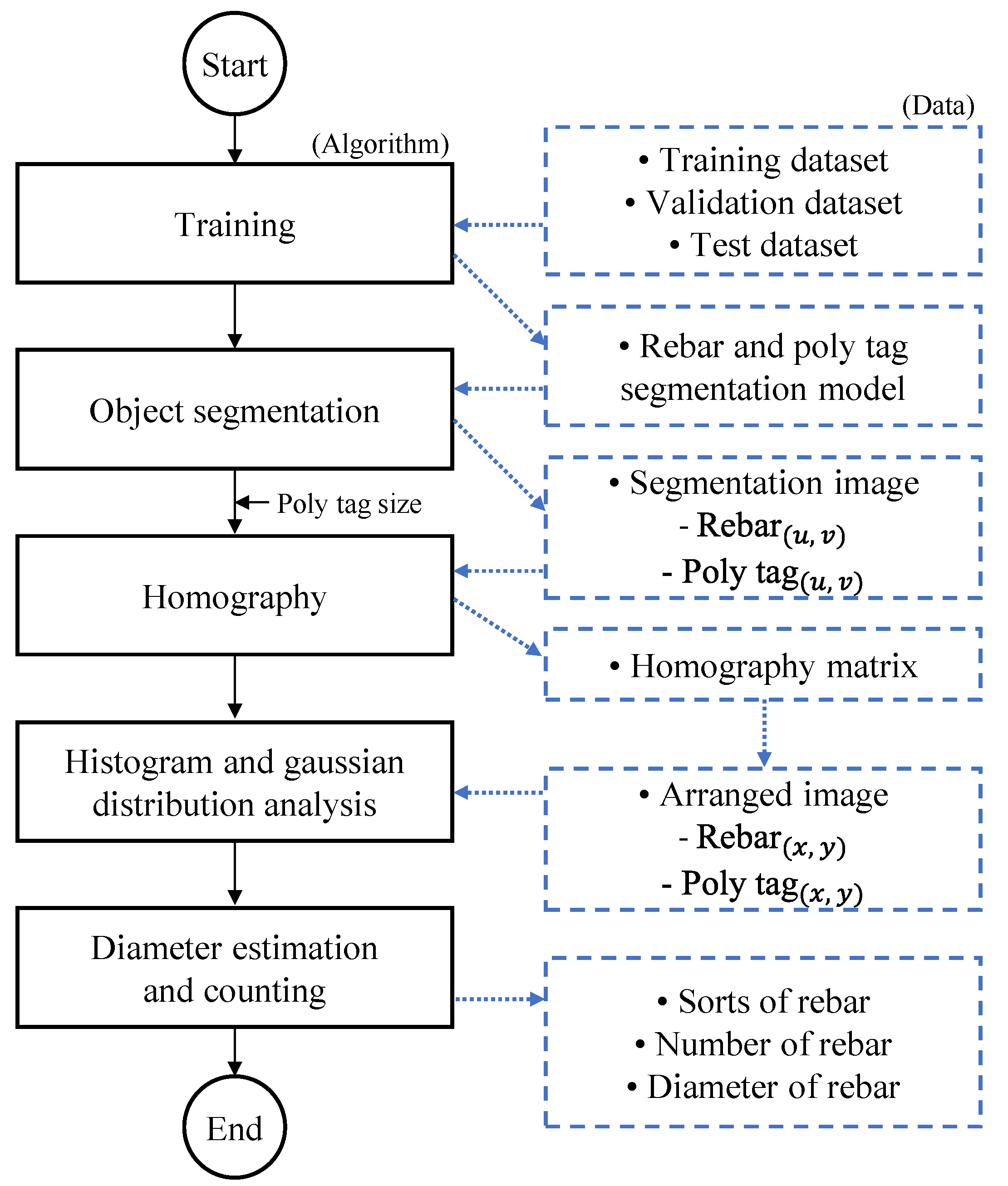
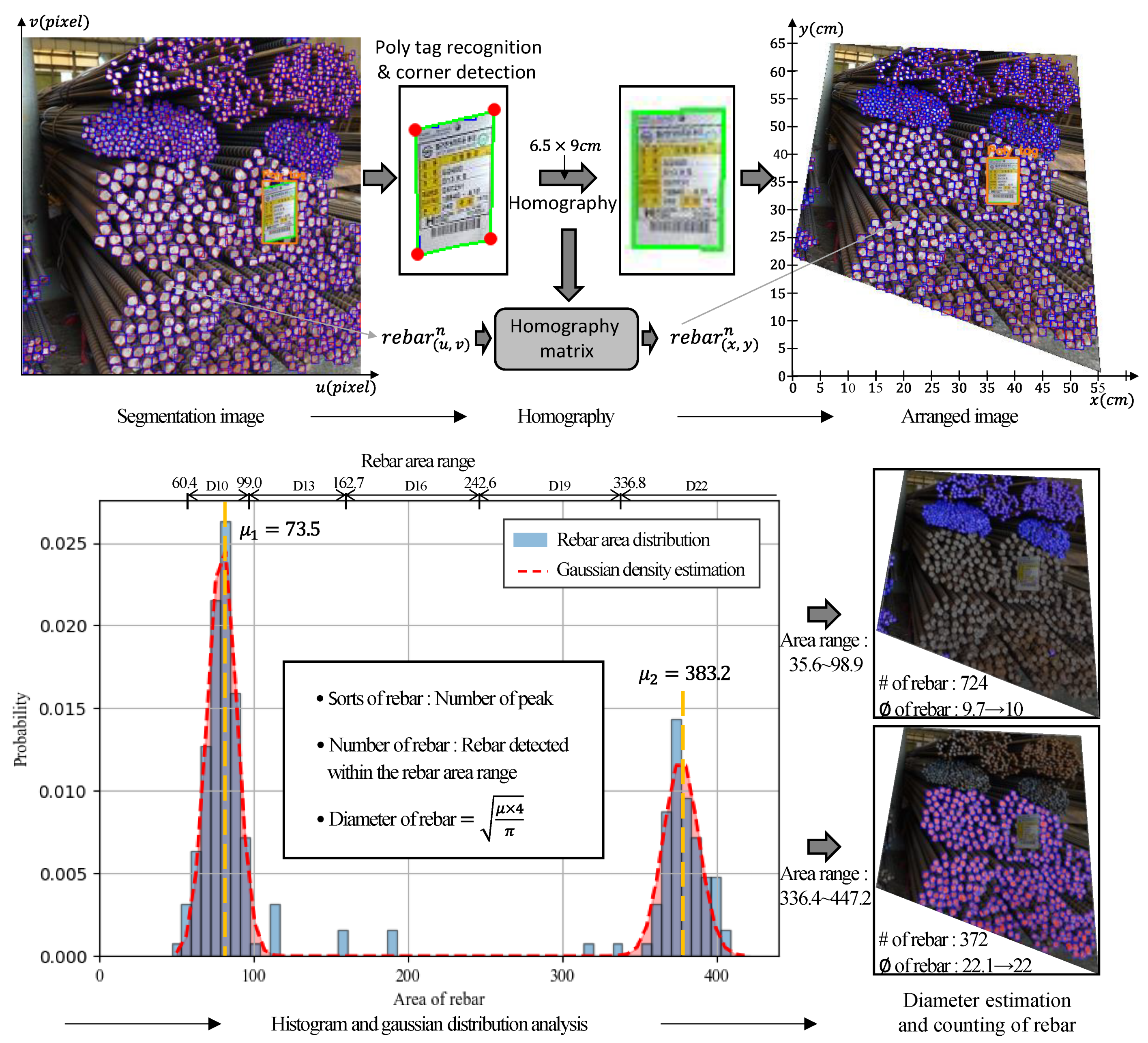
3.1. Research Method

While several studies have tried to count rebars by adopting various proposed CNN architectures to enhance accuracy and reduce inference time, they have only focused on counting the exact number of rebars rather than discerning their size as well, as discussed in the previous section. In this study, we developed an automated rebar counting and size estimation technique based on a convolutional neural network (CNN) and image processing for the efficient management of materials at construction sites or rebar manufacturing plants. Non-contact image sensing can cover multiple objects using a single camera and has better accessibility than other sensors, such as mobile phones. Additionally, CCTVs are already installed at construction sites for security and safety reasons. Hence, it is possible to apply the developed image-based technology without the need to install additional sensors.

Rebar counting and size estimation can each be achieved by the cross-sectional division of individual rebars in the image and the pixel range occupied by the cross section. Therefore, the acquisition of images that contain the cross section, and the detection and segmentation of the cross section of individual rebars need to be performed sequentially. Although the detection and segmentation of the cross section of individual rebars can be conducted through a CNN model, two other issues need to be addressed to perform rebar counting and size estimation: (1) A scale factor is required to apply the actual dimensions to the detection and segmentation coordinates composed of pixel coordinates. (2) In the case of an image captured from an oblique angle, the area of the near cross section and that of the far cross section are different, even for the same rebar. Computer-vision-based homography is effective in simultaneously solving these two issues.

Homography is an image processing that acquires an image from a virtual image-capturing angle through the transformation relationship between the corresponding points of two images [30,31,32,33,34]. Homography can transform a perspective of an image captured from an oblique direction into a front view image captured from the front direction (where the camera is facing the object directly). Generally, four corresponding points with known sizes are required to perform this transformation. However, poly tags of uniform dimensions are attached to piles of rebars, and they contain information such as the production time and rebar specifications. This information is utilized in homography to obtain the scale for the pixels and a virtual front view image.

The research process of rebar counting and size estimation consists of a five-step sequential algorithm, as shown in Figure 1. Firstly, a CNN model is created using images containing various rebar cross sections for object detection and instance segmentation. The dataset consists of a training dataset for training, a validation dataset to prevent overfitting, and a test dataset to verify the trained model. Secondly, the segmentation image is obtained by putting the images for rebar counting and size estimation in the generated CNN model. The segmentation image consists of rebars composed of (u, v), a perspective coordinate system, and each object of the poly tag is composed of polygons. Here, homography is applied to the entire image by entering the poly tag information in advance, and the rebars composed of (u, v) and the individual objects of the poly tag are converted into the (x, y) coordinate system of the actual scale through the homography matrix. Lastly, information on the converted rebars, such as the number of types of rebars in the image and the number and sizes of the rebars for each type, is obtained through a histogram and Gaussian distribution analysis.

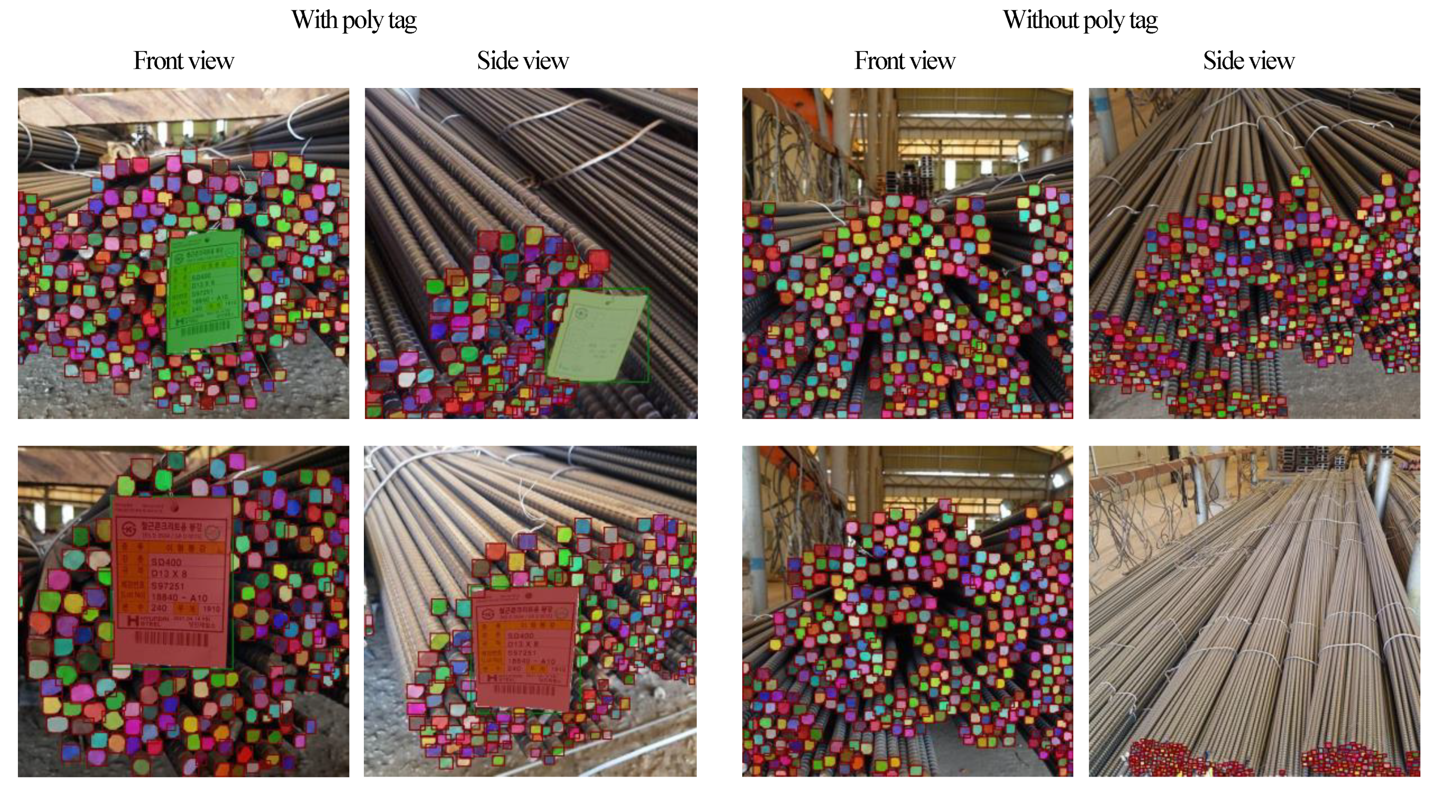
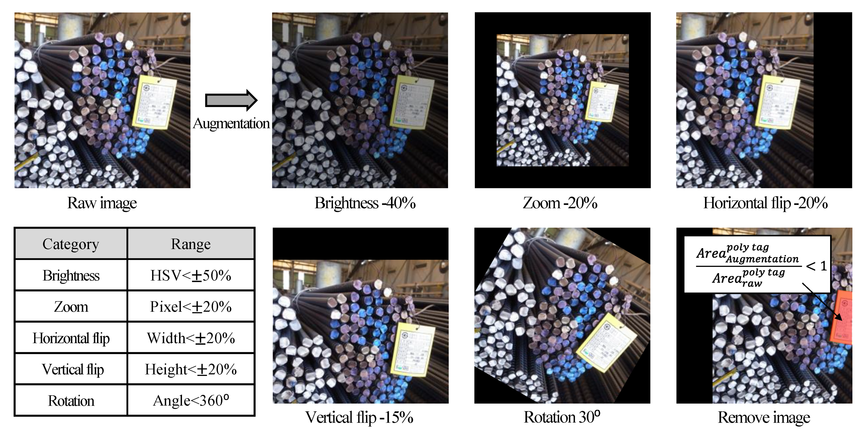
3.2. Image Acquisition for Instance Segmentation

Various studies have been conducted on object detection techniques that express the minimum range of the area containing the object using rectangular coordinates and instance segmentation techniques that represent the boundary of the object with a polygon to handle the objects in the image using a CNN model [19,25,35,36,37]. Generally, object detection expresses the position of the object using four coordinates, whereas instance segmentation uses tens to hundreds of coordinates to represent the boundary of the object, depending on the size of the image and the size and shape of the object. Although instance segmentation can accurately extract the boundary of the object, it consumes much time and computing resources compared with object detection. Hence, it is important to use a CNN model suitable for the purpose.

Pixels occupied by the rebar cross sections in the image are directly associated with the size of the rebars after applying homography. Therefore, pixels occupied by the cross sections of rebars must be segmented accurately. Instance segmentation of individual rebars represents the coordinates of the pixels for the corresponding rebar as a polygon. For CNN-based supervised learning instance segmentation, the coordinates of the edges of the target object to be segmented need to be annotated by a person. In this study, the annotation was performed on an image containing the rebar cross sections to be segmented and a poly tag, and was used as a dataset for generating the CNN model.

A dataset containing processed 622 images of rebars including a total of 186,522 rebar cross sections and 409 poly tags was established for segmentation rebars and poly tags in images. The images were collected in full HD resolution of 1920 × 1080 pixels and then center-cropped to 1080 × 1080 pixels. The cropped images were then down-sampled to 512 × 512 pixels to increase the computing speed. In the dataset, the number of rebar cross sections captured in a single image varies from approximately 50 to 1000. The annotation tool LabelMe [38] was used to assign the polygon ground-truth bounding boxes to the rebar cross sections, which is necessary for supervised learning procedures. Figure 2 shows representative raw images and a labeling of the ground truth. Of the 622 images, 409 images contained poly tags, but the remaining 213 images contained only rebar cross sections without poly tags. Images were taken from various angles, as well as from the front; up to four images were taken of the same pile of rebars. Of the 622 images, 498, 93, and 31 images (or 80%, 15%, and 5% of the images) were randomly classified into the train, validation, and test datasets, respectively. Additionally, some test dataset images were annotated on the original image of 1920 × 1080 pixels to improve the precision for minute objects, such as rebars of less than D10, adopting a machine learning model to enhance the accuracy with lowering the speed of object recognition.

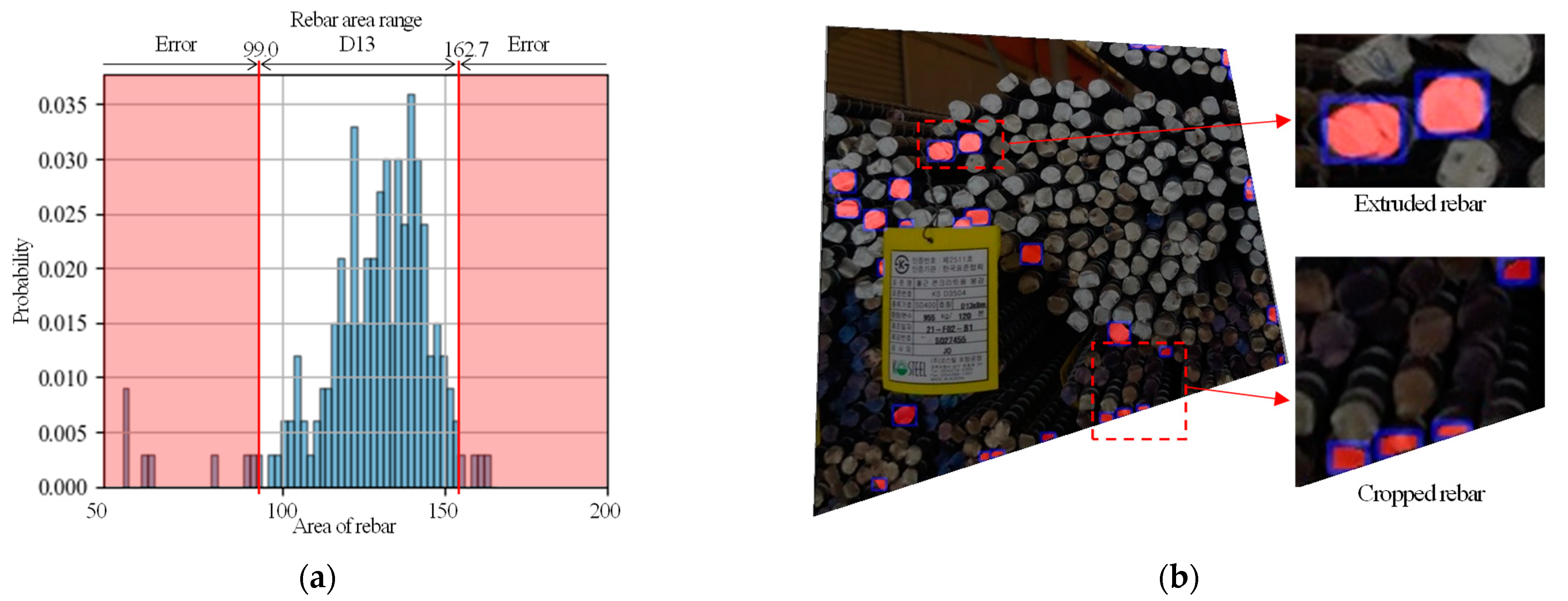
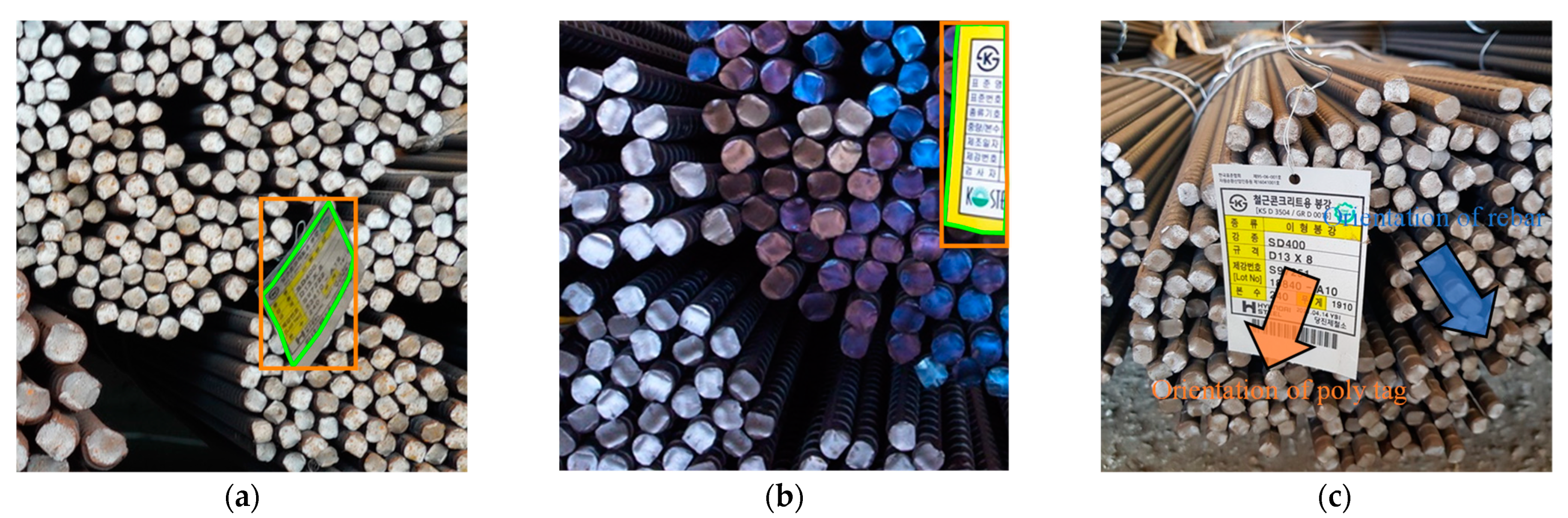
3.3. Rebar Size Estimation Using Homography

Figure 3 shows the detailed rebar counting and size estimation process, which is performed after the detection and segmentation of the rebars and poly tags are completed using the CNN model. Corner detection is applied to the poly tag extracted from the segmentation image; thus, four corresponding points to be used in homography are extracted. The poly tags used in this study have fixed dimensions of 6.5 cm × 9 cm in width and length and are input in the same size for all the homographic tasks. A poly tag photographed from an oblique direction is converted to the frontal direction through homography. At the same time, the horizontal and vertical pixels have an actual scale of 6.5 cm × 9 cm. The homography matrix created here is equally applied to the entire image and individual rebars, in addition to the poly tag, to obtain the polygon coordinates composed of the arranged image of the front view and the (x, y) coordinates of the actual scale.

The converted polygon area is the area of the corresponding rebar cross-section; hence, the Gaussian distribution analysis is performed on the histogram representing all polygon areas. Here, the number of peaks in the Gaussian distribution represents the types of the rebar size, and the x value $\mu$, which is the location of the peak, is the average of the group of rebar cross sections in the corresponding Gaussian distribution. The diameter of the rebar can be calculated through Equation (1).

$$d=\frac{\sqrt{\mu \times 4}}{\pi }$$

(1)

where, d is the diameter of the steel rebars (in mm), and μ is the peak value from the histogram and the Gaussian distribution analysis. The number of rebars for the corresponding size is the number of histogram samples within the proposed area range presented in

Table 1. Rebar standard in KS D3504:2021 [39] and the proposed area range for size estimation.

Type	Nominal Diameter (mm)	Nominal Cross Section Area (mm2)	Estimated Area (mm2, Proposed)
D10	9.53	71.33	Min	60.4
			Max	99.0
D13	12.7	126.7	Min	99.0
			Max	162.6
D16	15.9	198.6	Min	162.6
			Max	242.5
D19	19.1	286.5	Min	242.5
			Max	336.8
D22	22.2	387.1	Min	336.8
			Max	446.9
D25	25.4	506.7	Min	449.9
			Max	576.2

. Histogram samples in a range outside the rebar size types inferred in advance are classified as errors that occur during image processing. This is described in detail in Section 4 of this paper.

Because the sample image used in Figure 3 contains two types of rebars, two peaks were generated in the Gaussian distribution analysis. The x values of the two peaks, ${\mu }_1$ and ${\mu }_2$, are 73.5 $\mathrm{m}{\mathrm{m}}^2$ and 383.2 $\mathrm{m}{\mathrm{m}}^2$, respectively. The diameters of the two types of rebars are 9.7 mm and 22.1 mm, respectively. In other words, we can confirm that the two rebar types are the D10 and D22 rebars. Based on the proposed rebar area ranges in Table 1, 724 rebars were counted for D10 rebars, and 372 rebars were counted for the D22 rebars.

The existing standards reflect a certain delay in the advances of technology in product manufacturing with the growing requisites of the users. In the case of rebars, the ISO standards have not been widely adopted yet, and national standards are still predominant. In this paper, the Korea national standards, KS D3504:2021 [39], were applied for the diameter and area values according to the size of the rebars for the accurate comparison of the obtained data and the analysis results. Because KS D3504:2021 [39] refers to the international standards ISO 3534-1:2006 [40], and the US national standards ASTM A615 [41], the rebar notations and sizes are similar to the international standards. Rebars are classified into 18 types, from D4 to D57. The standards quantitatively present the nominal diameter and nominal cross-section area of the rebars, and some of them are listed in Table 1. Here, the average value of the nominal cross-section area of two consecutive rebar types was proposed as the estimated area to determine the size of the rebar obtained from the image. For example, the estimated area of D13 ranges from 99.0 to 162.6. Here, the minimum value of 99.0 is the average value of the area of D13 (126.7 mm²) and that of D10 (71.33 mm²), and the maximum value of 162.6 mm² is the average value of the area of D13 (126.7 mm²) and that of D16 (198.6 mm²).

4. Results

4.1. Training and Evaluation

In this section, we present the research results. The hardware for the algorithm testing used the NVIDIA GeForce RTX 2080 Ti Graphics Processing Unit (GPU). YOLACT [42] was used to create a CNN-based model that can segment the rebar cross sections and poly tags in the image. Transfer learning based on the pre-trained weights of the COCO dataset [43] and image processing-based data augmentation were performed. Transfer learning was first performed on a large dataset, and the pre-trained weights were then used for initialization or as fixed feature extractors for a new target task to improve learning accuracy. Transfer learning was performed in two steps: (1) The weights pre-trained on the COCO dataset are used to initialize the backbone and post-processing modules. Only the weight parameters of the post-processing module are then optimized based on the steel frame dataset. (2) The weight parameters of the entire network are restored, and they are fine-tuned using the same dataset.

Data augmentation aims to increase the variability of the same image to make the trained model robust to images obtained in different environments. Brightness, zoom, flip, and rotation techniques were randomly applied 10 times such that the same technique could be applied redundantly up to two times for an image. Brightness was applied within a $\pm 40\%$ range based on HSV (hue, saturation, and value), and zoom was applied within a 20% range of the maximum pixels. Flip was applied within a 20% range of the horizontal and vertical size, respectively, and rotation was applied within a 360° range around the center. The area ratio of the poly tag before and after data augmentation is calculated for these techniques, except for zoom. If the ratio becomes smaller than one, it indicates that a part of the poly tag is damaged. Consequently, that image is excluded from the training dataset. Figure 4 shows an example of each technique.

The data augmentation technique was applied to 498 images of the pre-configured training dataset, and a total of 4668 images were used for the final training. A total of 10,000 training iterations were performed on the dataset.

Table 2. mAP by YOLACT-based training.

Iteration		All	0.50	0.55	0.60	0.65	0.70	0.75	0.80	0.85	0.90	0.95
500	Box	19.86	38.10	60.51	26.30	23.30	18.95	15.67	11.60	11.42	6.24	2.48
	Mask	20.36	40.59	25.77	22.20	18.13	15.57	13.40	8.62	8.32	1.79	0.61
1000	Box	32.53	53.61	46.80	40.17	32.86	26.69	20.35	16.57	16.09	8.10	5.29
	Mask	31.98	58.38	42.17	35.12	27.25	21.63	18.87	12.86	11.56	2.33	0.83
5000	Box	33.24	55.74	48.06	40.40	33.88	28.10	20.98	17.26	16.58	8.53	5.56
	Mask	32.73	59.30	42.47	35.63	28.38	22.53	19.45	13.40	12.17	2.43	0.87
10,000	Box	33.21	56.32	48.53	41.05	34.22	28.67	21.19	17.61	16.75	8.70	5.62
	Mask	32.83	59.21	42.37	35.31	28.96	22.76	19.65	13.67	12.29	2.45	0.88

lists the mAP (mean average precision) for every 500, 1000, 5000 and 10,000 iterations for the two classes of steel rebars and poly tags over different IoU thresholds, from 0.5 to 0.95. In all the IoU ranges, mAPs greater than or equal to 50 were obtained for the Box and Mask in the 1000th iteration. Subsequently, a model with a Box of 52.21 and a Mask of 52.83 was obtained in the final, 10,000th iteration.

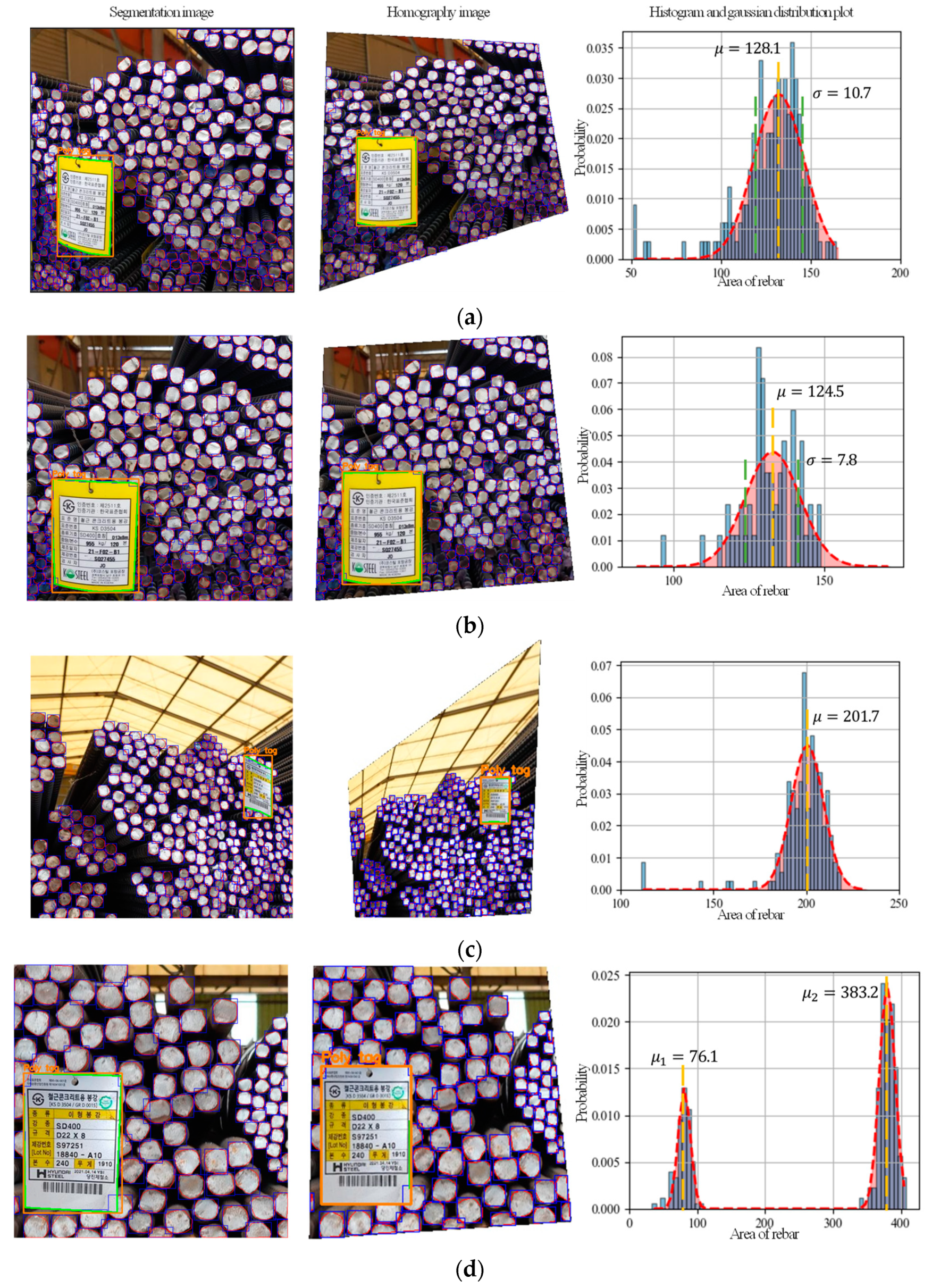
4.2. Rebar Size Estimation and Counting Results

Figure 5 presents the results of four sample images from the test dataset for rebar size estimation and counting. For each image, the segmentation image, which is the output of the segmentation model, the homography image by corner detection for poly tags, and the histogram and Gaussian distribution plot are sequentially listed.

Table 3. Details on the results of the samples.

Sample Image	Size (mm)		Count (the Number)		Error (%)
	Actual	Estimated	Actual	Estimated	Size	Count
Figure 5a	13	12.77	281	254	1.7	9.6
Figure 5b	13	12.59	219	207	3.1	4.5
Figure 5c	16	16.03	294	286	0.1	2.7
Figure 5d	10	9.85	27	29	1.5	7.4
	22	22.09	67	69	0.4	2.9

presents these results. The actual number of rebars is the number of annotations labeled by a person.

Figure 5a,b are images captured from the same pile of D13 size rebars. Figure 5a is the image taken from an oblique direction to the right, and Figure 5b is the image captured from the front direction. The Gaussian parameters mean $\mu$ and standard deviation $\sigma$ are $\mu =128.1$ and $\sigma =10.7$ in Figure 5a and are $\mu =124.5$ and $\sigma =7.8$ in Figure 5b. The diameters of the rebars calculated using $\mu$ are 12.77 and 12.59, respectively, and the error rates are 1.7% and 3.1%, respectively. Thus, the standard deviation of Figure 5b is 2.9 lower than that of Figure 5b. This result confirms that the image taken from the front direction has a more stable area distribution.

Figure 5c shows a pile of D16 rebars, and the poly tag size is approximately 1/30 of the image size. Thus, it is a sample image for a case when the homography target is very small. Similarly, the corner of the poly tag was recognized in this sample, and homography was performed smoothly. A result of $\mu =201.7$ with a size of 16.03 was obtained.

Figure 6b shows an image containing two types of rebars, D10 and D22. Two peaks were generated in the histogram and Gaussian distribution analysis, and the values of ${\mu }_1=76.1 and {\mu }_2=383.2$ were obtained. The size of each rebar type is 9.85 and 22.09, respectively, indicating highly accurate estimation.

Among the four sample images, Figure 5a shows the highest counting error. Consequently, an analysis was performed on the objects outside the rebar area range in Figure 5a, which are rebars that have been classified as errors. The rebar area range of the D13 rebars is 99.0 ${\mathrm{mm}}^2-$162.7 ${\mathrm{mm}}^2$. Hence, if the segmented polygon area is smaller than 99.0 ${\mathrm{mm}}^2$ or larger than 162.7 ${\mathrm{mm}}^2$, the corresponding rebar is not recognized as a D13 rebar, as shown Figure 6a. Figure 6b presents an image that only shows the rebars of the homography image that fall in the error range. If the area is larger than 162.7 ${\mathrm{mm}}^2$, it indicates that the projected rebar has occurred owing to uneven indentation. If the area is smaller than 99.0 ${\mathrm{mm}}^2$, it indicates that a part of the rebar has been cut off the edge of the image or the poly tag. From this analysis, it was inferred that the rebar pile should be arranged neatly to reduce the counting error occurrence rate, or that the picture should be taken in a way to ensure all rebars are included in the image.

Figure 7 shows the images for which the size estimation was not performed properly. Figure 7a shows a case where the poly tag is detached from the rebars or is deformed. In such cases, the poly tag could be recognized, but corner detection failed in most cases. Even when the corner detection succeeded, homography could not be performed properly. Figure 7b is an image where a part of the poly tag is cut off. Although corner detection is possible, homography is applied with an incorrect size because the size of the poly tag input has been set to 6.5 cm × 9 cm in advance. For Figure 7c, the orientations of the rebar and the poly tag do not match because the poly tag was not attached to the rebars correctly. In this case, while poly tag recognition, corner detection, and homography are properly performed, the cross section of the rebar is not aligned to the front view. This misalignment leads to a difference in the area due to perspective, although the rebars are the same size. Consequently, the rebar size is estimated incorrectly. Therefore, to apply the size estimation technique developed in this study, a poly tag that is not cut off or deformed has to be attached in the direction matching the orientation of the rebars.

5. Conclusions

Steel rebars are a significant construction material in the reinforced concrete structures due to its superb mechanical properties as well as the proportion of the construction costs over the complete structure. While the manual rebar counting is a common practice at the construction sites, it entails several drawbacks: it is human-resource-intensive, time-consuming, error-prone, and possibly injurious. In this study, the authors developed an automated system to estimate the size and count the number of steel rebars in bale packing based on CNN-based computer vision techniques. The results of this research show the following:

• The proposed method, a CNN model combined with homography, can estimate the size and count the number of steel rebars in an image quickly and accurately, and the method can be applied to real construction sites to manage the stock of steel rebars efficiently.
• The application of a homography image by corner detection for poly tags as well as a histogram and Gaussian distribution plot can be used to effectively estimate the size and count the number of steel rebars from images with different perspectives.
• In this study, 622 images taken at various angles and that include a total of 182,522 steel rebars were manually labeled to create the dataset. Data augmentation was carried out to create 4668 images for the training dataset. Based on the training dataset, YOLACT-based steel bar size estimation and a counting model with a Box and Mask of over 30 mAP was generated to satisfy the aim of this study.
• The test results show that the maximum error rate for estimating the size and counting the number of steel rebars in an image was 3.1% and 9.6%, respectively. Most of the errors shown in this study were caused by images of steel rebars whose edges were cut off or that suffered from uneven indentation.

While the proposed method in this study shows an acceptable level of performance, the error rate in estimating the size and counting the number of steel rebars should be improved for practical applications of complicated real construction sites. Moreover, application of the proposed method must be expanded, e.g., to H-beam, channels, angles, and pipes in order to efficiently manage construction materials at construction sites.

References

1. MacGregor, J.G.; Wight, J.K. Reinforced Concrete: Mechanics and Design, 6th ed.; Prentice Hall Upper: Saddle River, NJ, USA, 1997; Volume 3. [Google Scholar]
2. Na, S.; Paik, I. Application of Thermal Image Data to Detect Rebar Corrosion in Concrete Structures. Appl. Sci. 2019, 9, 4700. [Google Scholar] [CrossRef] [Green Version]
3. Kmiecik, P.; Kamiński, M. Modelling of reinforced concrete structures and composite structures with concrete strength degradation taken into consideration. Arch. Civ. Mech. Eng. 2011, 11, 623–636. [Google Scholar] [CrossRef]
4. Kaming, P.F.; Olomolaiye, P.O.; Holt, G.; Harris, F.C. Factors influencing construction time and cost overruns on high-rise projects in Indonesia. Constr. Manag. Econ. 1997, 15, 83–94. [Google Scholar] [CrossRef]
5. Duggal, S.K. Building Materials; Routledge: London, UK, 2017. [Google Scholar]
6. Kodur, V.; Harmathy, T. Properties of building materials. In SFPE Handbook of Fire Protection Engineering; Springer: Cham, Switzerland, 2016; pp. 277–324. [Google Scholar]
7. Allen, E.; Iano, J. Fundamentals of Building Construction: Materials and Methods; John Wiley & Sons: Hoboken, NJ, USA, 2019. [Google Scholar]
8. Kim, M.-K.; Thedja, J.P.P.; Chi, H.-L.; Lee, D.-E. Automated rebar diameter classification using point cloud data based machine learning. Autom. Constr. 2021, 122, 103476. [Google Scholar] [CrossRef]
9. Zhang, D.; Xie, Z.; Wang, C. Bar Section Image Enhancement and Positioning Method in On-Line Steel Bar Counting and Automatic Separating System. In Proceedings of the 2008 Congress on Image and Signal Processing, Washington, DC, USA, 27–30 May 2008; Institute of Electrical and Electronics Engineers (IEEE): Piscataway, NJ, USA, 2008; Volume 2, pp. 319–323. [Google Scholar]
10. Zhu, Y.; Tang, C.; Liu, H.; Huang, P. End-Face Localization and Segmentation of Steel Bar Based on Convolution Neural Network. IEEE Access 2020, 8, 74679–74690. [Google Scholar] [CrossRef]
11. Ying, X.; Wei, X.; Pei-Xin, Y.; Qing-Da, H.; Chang-Hai, C. Research on an Automatic Counting Method for Steel Bars’ Image. In Proceedings of the 2010 International Conference on Electrical and Control Engineering, Washington, DC, USA, 25–27 June 2010; Institute of Electrical and Electronics Engineers (IEEE): Piscataway, NJ, USA, 2010; pp. 1644–1647. [Google Scholar]
12. Hernández-Ruiz, A.; Martínez-Nieto, J.A.; Buldain-Pérez, J.D. Steel Bar Counting from Images with Machine Learning. Electronics 2021, 10, 402. [Google Scholar] [CrossRef]
13. Xia, Y.; Shi, X.; Song, G.; Geng, Q.; Liu, Y. Towards improving quality of video-based vehicle counting method for traffic flow estimation. Signal Process. 2016, 120, 672–681. [Google Scholar] [CrossRef]
14. Sindagi, V.A.; Patel, V.M. A survey of recent advances in CNN-based single image crowd counting and density estimation. Pattern Recognit. Lett. 2018, 107, 3–16. [Google Scholar] [CrossRef] [Green Version]
15. Sun, M.; Wang, Y.; Li, T.; Lv, J.; Wu, J. Vehicle counting in crowded scenes with multi-channel and multi-task convolutional neural networks. J. Vis. Commun. Image Represent. 2017, 49, 412–419. [Google Scholar] [CrossRef]
16. Shen, J.; Xiong, X.; Xue, Z.; Bian, Y. A convolutional neural-network-based pedestrian counting model for various crowded scenes. Comput. Aided Civ. Infrastruct. Eng. 2019, 34, 897–914. [Google Scholar] [CrossRef]
17. Asadi, P.; Gindy, M.; Alvarez, M. A Machine Learning Based Approach for Automatic Rebar Detection and Quantification of Deterioration in Concrete Bridge Deck Ground Penetrating Radar B-scan Images. KSCE J. Civ. Eng. 2019, 23, 2618–2627. [Google Scholar] [CrossRef]
18. Wang, C.; Zhang, H.; Yang, L.; Liu, S.; Cao, X. Deep People Counting in Extremely Dense Crowds. In Proceedings of the 23rd ACM international conference on Multimedia, Brisbane, Australia, 26–30 October 2015; Association for Computing Machinery: New York, NY, USA, 2015; pp. 1299–1302. [Google Scholar]
19. Miikkulainen, R.; Liang, J.; Meyerson, E.; Rawal, A.; Fink, D.; Francon, O.; Raju, B.; Shahrzad, H.; Navruzyan, A.; Duffy, N.; et al. Evolving Deep Neural Networks. In Artificial Intelligence in the Age of Neural Networks and Brain Computing; Elsevier: Amsterdam, The Netherlands, 2019; pp. 293–312. [Google Scholar]
20. Sam, D.B.; Surya, S.; Babu, R.V. Switching Convolutional Neural Network for Crowd Counting. In Proceedings of the 2017 IEEE Conference on Computer Vision and Pattern Recognition (CVPR), Honolulu, HI, USA, 21–26 July 2017; pp. 4031–4039. [Google Scholar]
21. Ilyas, N.; Shahzad, A.; Kim, K. Convolutional-Neural Network-Based Image Crowd Counting: Review, Categorization, Analysis, and Performance Evaluation. Sensors 2019, 20, 43. [Google Scholar] [CrossRef] [PubMed] [Green Version]
22. Li, Y.; Zhang, X.; Chen, D. CSRNet: Dilated Convolutional Neural Networks for Understanding the Highly Congested Scenes. In Proceedings of the 2018 IEEE/CVF Conference on Computer Vision and Pattern Recognition, Salt Lake City, UT, USA, 18–23 June 2018; pp. 1091–1100. [Google Scholar]
23. Gomaa, A.; Abdelwahab, M.M.; Abo-Zahhad, M.; Minematsu, T.; Taniguchi, R.-I. Robust Vehicle Detection and Counting Algorithm Employing a Convolution Neural Network and Optical Flow. Sensors 2019, 19, 4588. [Google Scholar] [CrossRef] [Green Version]
24. Khaki, S.; Safaei, N.; Pham, H.; Wang, L. Wheatnet: A lightweight convolutional neural network for high-throughput image-based wheat head detection and counting. arXiv 2021, arXiv:2103.09408. [Google Scholar]
25. Walach, E.; Wolf, L. Learning to count with CNN boosting. In European Conference on Computer Vision; Springer: Cham, Switzerland, 2016. [Google Scholar]
26. Abdelwahab, M.A. Accurate Vehicle Counting Approach Based on Deep Neural Networks. In Proceedings of the 2019 International Conference on Innovative Trends in Computer Engineering (ITCE), Aswan, Egypt, 2–4 February 2019; Institute of Electrical and Electronics Engineers (IEEE): Piscataway, NJ, USA, 2019; pp. 1–5. [Google Scholar]
27. Chung, J.; Kim, G.; Sohn, K. Transferability of a Convolutional Neural Network (CNN) to Measure Traffic Density. Electronics 2021, 10, 1189. [Google Scholar] [CrossRef]
28. Fan, Z.; Lu, J.; Qiu, B.; Jiang, T.; An, K.; Josephraj, A.N.; Wei, C. Automated steel bar counting and center localization with convolutional neural networks. arXiv 2019, arXiv:1906.00891. [Google Scholar]
29. Li, Y.; Lu, Y.; Chen, J. A deep learning approach for real-time rebar counting on the construction site based on YOLOv3 detector. Autom. Constr. 2021, 124, 103602. [Google Scholar] [CrossRef]
30. Dubrofsky, E. Homography Estimation. Diplomová Práce; Univerzita Britské Kolumbie: Vancouver, BC, Canada, 2009; Volume 5, Available online: https://citeseerx.ist.psu.edu/viewdoc/download?doi=10.1.1.186.5926&rep=rep1&type=pdf (accessed on 1 September 2021).
31. DeTone, D.; Malisiewicz, T.; Rabinovich, A. Deep image homography estimation. arXiv 2016, arXiv:1606.03798. [Google Scholar]
32. Sukthankar, R.; Stockton, R.G.; Mullin, M.D. Smarter presentations: Exploiting homography in camera-projector systems. In Proceedings of the Eighth IEEE International Conference on Computer Vision, ICCV 2001, Vancouver, BC, Canada, 7–14 July 2001; Institute of Electrical and Electronics Engineers (IEEE): Piscataway, NJ, USA, 2002. [Google Scholar]
33. Benhimane, S.; Malis, E. Homography-based 2D Visual Tracking and Servoing. Int. J. Robot. Res. 2007, 26, 661–676. [Google Scholar] [CrossRef]
34. Malis, E.; Vargas, M. Deeper Understanding of the Homography Decomposition for Vision-Based Control. INRIA. 2007. Available online: https://hal.inria.fr/inria-00174036/ (accessed on 1 September 2021).
35. Albawi, S.; Mohammed, T.A.; Al-Zawi, S. Understanding of a convolutional neural network. In Proceedings of the 2017 International Conference on Engineering and Technology (ICET), Antalya, Turkey, 21–23 August 2017; pp. 1–6. [Google Scholar]
36. Lawrence, S.; Giles, C.L.; Tsoi, A.C.; Back, A.D. Face recognition: A convolutional neural-network approach. IEEE Trans. Neural Netw. 1997, 8, 98–113. [Google Scholar] [CrossRef] [PubMed] [Green Version]
37. Lin, X.; Zhao, C.; Pan, W. Towards accurate binary convolutional neural network. arXiv 2017, arXiv:1711.11294. [Google Scholar]
38. Russell, B.C.; Torralba, A.; Murphy, K.P.; Freeman, W.T. LabelMe: A Database and Web-Based Tool for Image Annotation. Int. J. Comput. Vis. 2008, 77, 157–173. [Google Scholar] [CrossRef]
39. Korea Agency for Technology and Standards. KS D 3504: 2021 Steel Bars for Concrete Reinforcement; Korea Standards and Certifications: Seoul, Korea, 2021. [Google Scholar]
40. International Organization for Standardization. ISO 3534-1:2006 Statistics–Vocabulary and Symbols—Part 1: General Statistical Terms and Terms Used in Probability; International Organization for Standardization: Geneva, Switzerland, 2016. [Google Scholar]
41. ASTM Standards. ASTM A615/A615M-20: Standard Specification for Deformed and Plain Carbon-Steel Bars for Concrete Reinforcement; ASTM Standards: West Conshohocken, PA, USA, 2020. [Google Scholar]
42. Bolya, D.; Zhou, C.; Xiao, F.; Lee, Y.J. Yolact: Real-Time Instance Segmentation. In Proceedings of the 2019 IEEE/CVF International Conference on Computer Vision (ICCV), Seoul, Korea, 27 October–2 November 2019. [Google Scholar]
43. Lin, T.-Y.; Maire, M.; Belongie, S.; Hays, J.; Perona, P.; Ramanan, D.; Dollár, P.; Zitnick, C.L. Microsoft COCO: Common Objects in Context. In Computer Vision—ECCV 2014; Fleet, D., Pajdla, T., Schiele, B., Tuytelaars, T., Eds.; Springer: Cham, Switzerland, 2014. [Google Scholar]
Figure 1. Flow chart for estimating the number and size of steel rebars.
Buildings 11 00463 g001
Figure 2. Representative raw images with annotations.
Buildings 11 00463 g002
Figure 3. Rebar size estimation and the counting process using homography.
Buildings 11 00463 g003
Figure 4. Data augmentation applied to images.
Buildings 11 00463 g004
Figure 5. Sample results of rebars. (a) Sample image on a pile of single type rebars take from an oblique angle. (b) Sample image on the sample pile of rebars shown in (a) taken from the from direction. (c) Sample image on a pile rebars to which a small poly tag is attached. (d) Sample image on a pile of two types of rebars.
Buildings 11 00463 g005
Figure 6. Sample analysis outside the rebar area range. (a) Histogram analysis and error range outside the D13 rebar area range. (b) Sample rebars observed in the error range.
Buildings 11 00463 g006
Figure 7. Cases of failure in rebar size estimation. (a) Poly tag detached or deformed. (b) Poly tag is cut off. (c) Orientation mismatch.
Buildings 11 00463 g007