1. Introduction
Friction stir welding is one of the most energy efficient processes and as such today has a great industrial application. It is used in all branches of industry, and primarily in space, aviation, shipbuilding, and rail industry. It features characteristics of an extremely good welded joint, the possibility of welding the plates of larger thicknesses, and the most important feature is the welding of dissimilar materials. Friction stir welding (FSW) was invented at the Welding Institute (TWI) of the United Kingdom in 1991 as a solid-state joining technique and was initially applied to aluminum-alloys [
1,
2,
3,
4,
5]. The process is carried out by using a tool of a cylindrical shape. The tool consists of two concentric parts of different diameters. A part of the tool of the larger diameter is called the shoulder, while a smaller diameter part is called a pin and is cone-shaped [
1,
2,
3,
4,
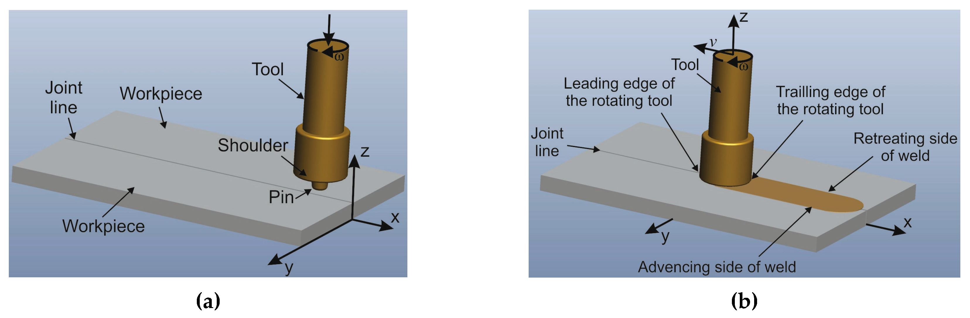
5]. The tool rotates at a high speed. The process FSW can be divided into two phases (
Figure 1). In the first phase, the tool moves axially and plunges into the material. During this, the heat from the friction is generated between workpieces and the surface of the tool pin and due to the plastic deformation of the material. When the shoulder reaches the surface of the workpiece and the tool begins to move longitudinally, the second phase, or phase of the welding of the material, begins [
5]. During this phase, in addition to the previously mentioned heat sources, most of the heat is obtained due to shoulder friction on the surface of workpieces [
5]. Thus, on the heat generation, the greatest influence has geometric parameters of the tool (shoulder diameter, pin diameter, and angle of pin slopes), which define the quality of the welded joint with the kinematic parameters (welding speed and rotation speed of tool). Therefore, these most influential parameters are the subject of our research.
As experimental research from real material is expensive, numerical experiments through the use of various software packages have shown that data obtained very successfully describes the studied process. Therefore, in a large number of published papers, numerical simulations of the FSW process are performed.
The paper [
6] deals with thermo-mechanical modeling and force analysis in the FSW process using the finite element method. When welding the sheet which is fixed in the rotating longitudinal movement of the tool using a mechanical force that is broken in three directions and combined with a temperature impact, deformation is caused and a solid welded joint is made. The natural assumption is that force control in FSW technology is important from the economic point of view, the aspect of productivity and the quality of welding. In order to design the FSW methodology, it is necessary to know the mechanical force, the speed of tool rotation, the longitudinal speed, the depth of the penetration of the tool into the material, and the thermo-mechanical properties of the material. This paper presents a three-dimensional model that is based on the method of finite elements for the distribution of temperature and stresses, taking into account the mechanical effects of the tool. Accordingly, a study of axial, longitudinal, and side forces is presented here in the process of welding aluminum alloy 6061. The welding process is simulated using a commercial package of finite elements ANSYS.
The paper [
7] presents an attempt to model the FSW process using a three-dimensional visco-plastic model. The field of this paper is focused on joining a thick aluminum sheet. The numerical model represents the successful design of the welding tools, which will produce the desired thermal gradient and prevent the breaking of the tools. Simulation of the welding process FSW with the finite element method was done using commercial FIDAP software (v7.6, Evanston, IL, USA).
The FSW method [
8] with stainless steel procedure was modeled using Euler’s formulation. Coupled high-viscous flow and a heat transfer of tool’s pin are considered. Model equations were solved using the finite element method in determining the speed and field of temperature distribution.
In the paper [
9], a two-dimensional simulation of the FSW process was performed, using finite elements and different ABAQUS options. The FSW process simulation focuses on the area of speed and characteristics of material flow.
When it comes to modeling the FSW process, great efforts are being made to understand the physical basis of the process through the study of experimental research.
The most commonly used software in modeling and numerical simulations in FSW friction welding processes are: ANSYS [
6], FIDAP [
7], ABAQUS [
9,
10,
11], MATLAB [
12], STIR3D [
13], and DEFORM [
14,
15].
The paper [
15] refers to the modeling of the FSW process, by using a commercially available nonlinear finite element (FE) code DEFORM. Temperature distribution, residual stress, strain and strain rates were analyzed in different regions of the welded joint.
Numerical modeling of FSW takes into account the thermal history [
7,
15,
16,
17,
18], the microstructure [
12], and the flow of materials [
7,
17,
18,
19]. Different numerical modeling approaches, such as finite elements [
7,
10,
16,
17] or final differences [
12,
20], have been used. These models were applied in determining the significance of the transmission effects, the prediction of local deformations [
12], simulating the appearance of the dissolution of the sediment along the grain boundaries [
20], determining the dependence of material viscosity on the temperature and process parameters [
19], calculating the pressure and velocity and connection of the process parameters with temperature and force on the tool [
7]. A certain group of materials has been taken into consideration, such as AA7050-T7451 [
7], AA2195-T8 [
10], AA6082.05-T6 and AA7108.50-T79 [
12], Ti-6Al-4V and AA1100 [
15], AA5454-O [
18], and AA6061-T6 [
19].
In the paper [
3], the influence of the tool’s angle of pin slope on the generated heat and material flow is researched. The effect of the tilt angle on the FSWelds is modeled through the contact condition by modifying an enhanced friction model. The mechanical effects caused by the tool tilt angle are presented in terms of velocity, stresses and strain rate fields, and material flow around the tool.
In the paper [
4], welding of dissimilar materials 2017A-T451 and 7075-T651 was performed. An existing computational model of the welding process for temperature distribution and material flow was adapted to estimate the phase transformations that occur in the weld zone. The phase transformation maps predicted by the simulation correlate with the hardness profiles and positron lifetime curves taken over the weld zone from the weld center (nugget) through the TMAZ to the HAZ.
The paper [
21] deals with the research of the metallurgical and microstructural aspects of FSW in terms of grain size and microhardness. The modeling is based on a combination of an apropos kinematic framework for local simulation of FSW processes and a material particle tracing technique for tracking the material flow during the weld. The resulting grain size and microhardness values are validated with experimental observations from an identical processed sample.
One of the most commonly used programs for volume deformation processes is the DEFORM package with multiple modules. DEFORM is based on the finite element method (FEM). For the numerical simulations in this research, the DEFORM 3D module was used.
2. Experimental Research
The machine used for the FSW process is a universal milling machine (6P13, GZFS, Russia), of a large stiffness. The milling machine has a movable working table of size 1500 mm × 300 mm, with the possibility of adjusting the stroke speed (mm/min), as well as the speed of the main spindle (rpm). The weight of the machine is 3500 kg and the motor power is 10 kW.
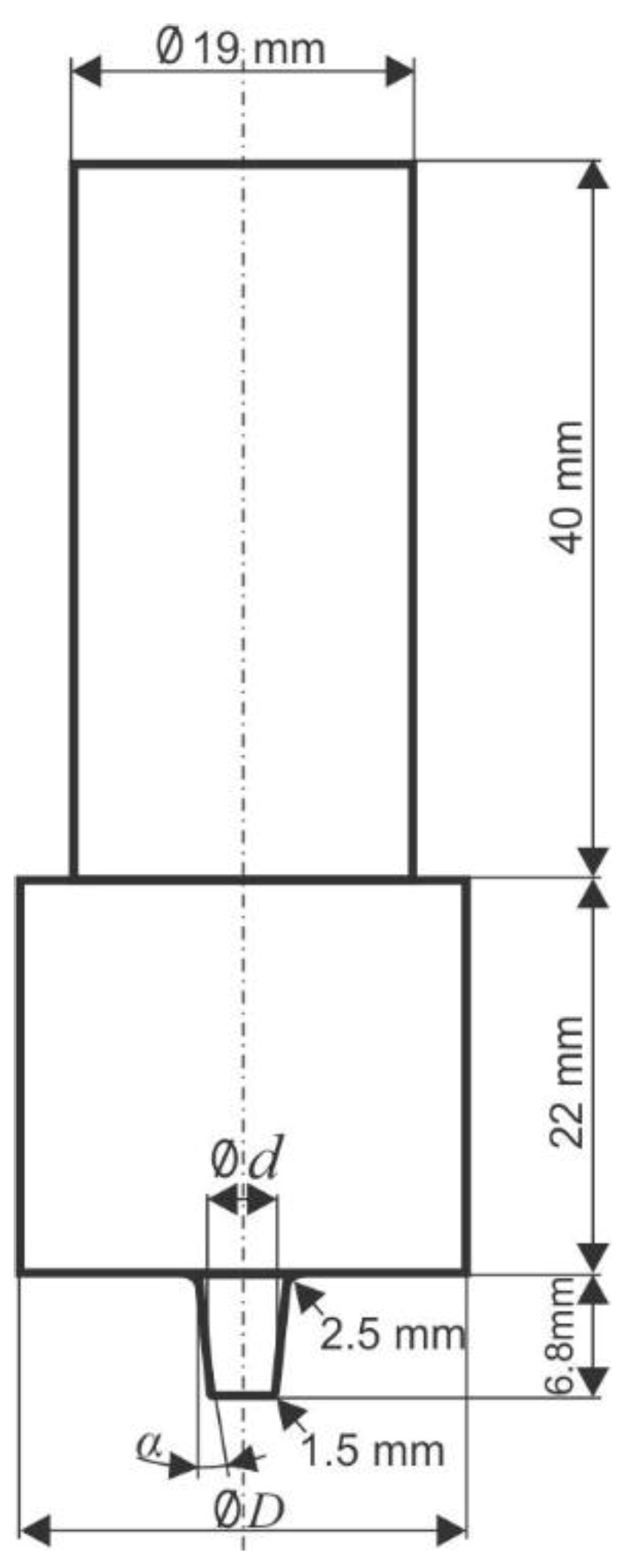
The material used in the experimental research is aluminum alloys AA6082-T6 with the thickness of 7.8 mm. This alloy has a great industrial application due to its good mechanical properties and relatively light weldability. For the experiment purposes, workpieces of 200 mm × 50 mm × 7.8 mm were made. For the welding process, the simple geometric shape tool is given in
Figure 2. The FSW process is achieved at a constant welding speed [
22].
For experimental research, the experiment plan was adopted and the input factors on the basis of which the output sizes were monitored. For the experiment plan, a complete five-factor orthogonal plan was adopted with a variety of factors on two levels and repetition at the central point of the plan
n0 = 4. The total number of experimental points is determined by the expression:
According to Equation (1), the number of experimental points is
N = 36, for the number of factors
k = 5. In order to determine the output size (
Y), the boundaries of the variation interval must be adopted so that the condition is satisfied:
where is:
—the value of the i-th factor at the upper level,
—the value of the i-th factor at the lower level,
—the value of the i-th factor at the basic level.
This condition applies to orthogonal plans. The
i-th factor levels are encoded by the transformation equation:
where they are:
—the natural value of the
i-th factor and,
—the factor variation interval whose numerical value is equal to the difference between the upper and the basic levels, ie the base and lower levels.
Geometric and kinematic parameters are applied as input quantities:
mm/min—welding speed,
rpm—rotation speed of tool,
0—the angle of pin slope,
mm—tool pin diameter,
mm—tool shoulder diameter.
Taking into account Equation (2), the adopted levels of input factor variation are given in
Table 1.
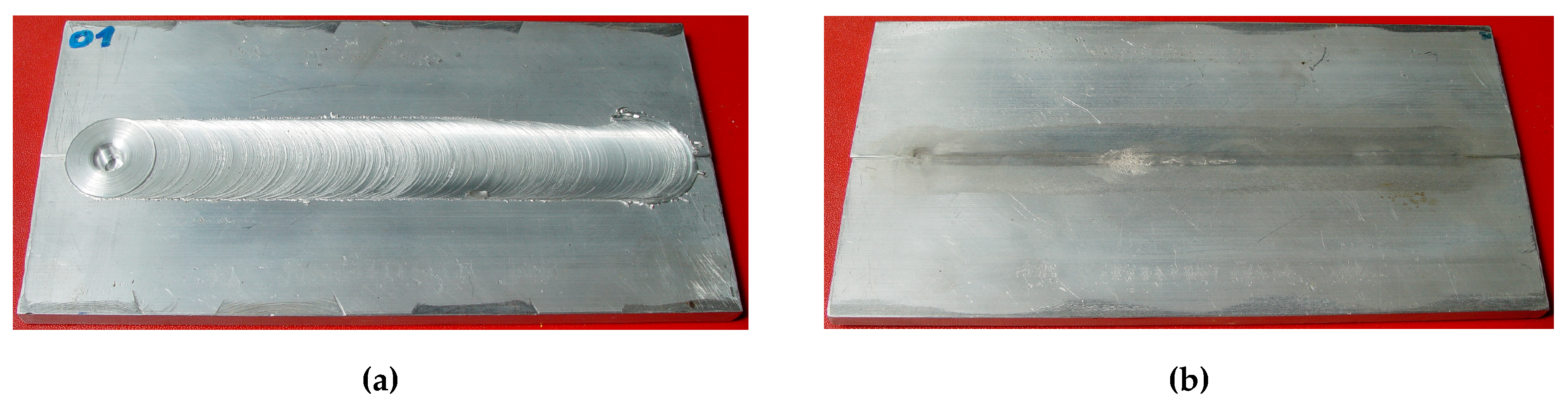
For the research needs, a set of 9 tools which geometric values were varied according to the adopted experiment plan. Also, 72 workpieces were produced, which are joined by the FSW process in 36 experimental points. In
Figure 3, the obtained welded compound is shown in experimental point number 1.
3. Numerical Simulation
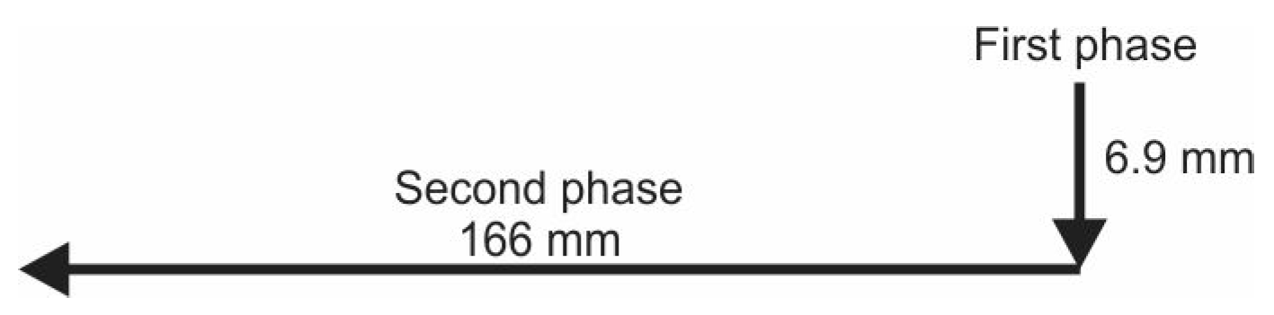
Using the DEFORM 3D (v5.0, SFTC, Columbus, OH, USA) software package, numerical simulations were performed. Tools and workpieces are generated in the CAD software CREO (v5.0, PTC, Boston, MA, USA). In order to be able to compare the obtained results with real conditions, 36 numerical simulations were performed based on the adopted experimental plan. Numerical simulation for each point of the experimental plan can be divided into two phases consisting of two stages (
Figure 7). In the first phase, the pin tool moves axially and plunges into the material at a depth of 6.9 mm and a shoulder of the tool at 0.1 mm, at a speed of
v = 30 mm/min. In the second phase, the tool moves longitudinally 166 mm, adopted at varying speeds
vu = 200 mm/min,
vl = 80 mm/min and
vb = 125 mm/min.
The DEFORM-3D module contains data that corresponds to the value of the real experiment. In submodule Simulation Control, the data related to the choice of system units are entered, the number of simulation steps, step increment to save, as well as the values of the termination process —SMAX. In the submodule Material, the data related to the material of the workpiece are entered. The ALUMINIUM-6082 material is selected whose parameters are in the database of DEFORM-3D which is defined:
where:
- flow stress,
- effective plastic strain,
- effective strain rate, and
T - temperature.
In the submodule Mesh, the number of 40,000 elements is selected, which is generated on the workpieces, and the submodule Movement contains values of moving speed tools (welding speed) and angular velocity (rotation speed of tool). For the first phase in the submodule Movement, the tool speed 0.5 mm/sec in the direction of “−z” (Constant) and in submodule Rotation1 angular velocity 83.78 Rad/sec in the direction of “−z” (Constant) are entered. In the second phase, the basic plate is the primary die and its speed corresponds to the point of the experimental plan, in this case, 2.0833 mm/sec which corresponds to the speed of 125 mm/min. At this phase, the tool speed is 0 mm/sec, and the angular velocity 83.78 Rad/sec, which corresponds to the rotation speed of the tool of 800 rpm [
22].
In the Inter-Object submodule (
Table 2) data are given relating to the relationship between the mold and the workpiece, as well as the friction factor and the heat transfer coefficient.
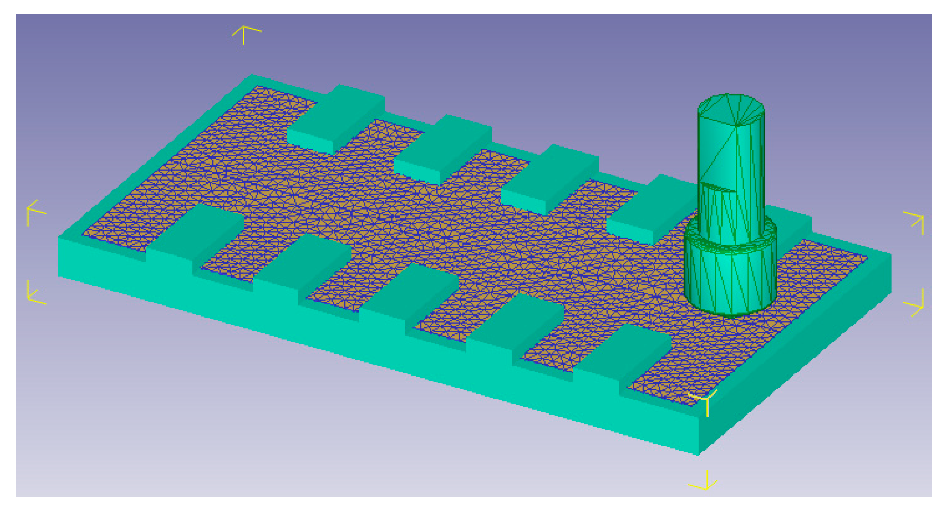
Other parameter values are taken as the default values of the software package DEFORM-3D. After entering the input data and generating the finite element mesh, the initial database for the initial step is formed, referred to as −1. When a database is formed, then all necessary requirements are met in order to perform the simulation of the FSW process. After the simulation, the results can be interpreted in the module Post Processor in the data and graphical form.
Figure 8 shows a 3D preview of workpieces with the generated finite element mesh [
22].
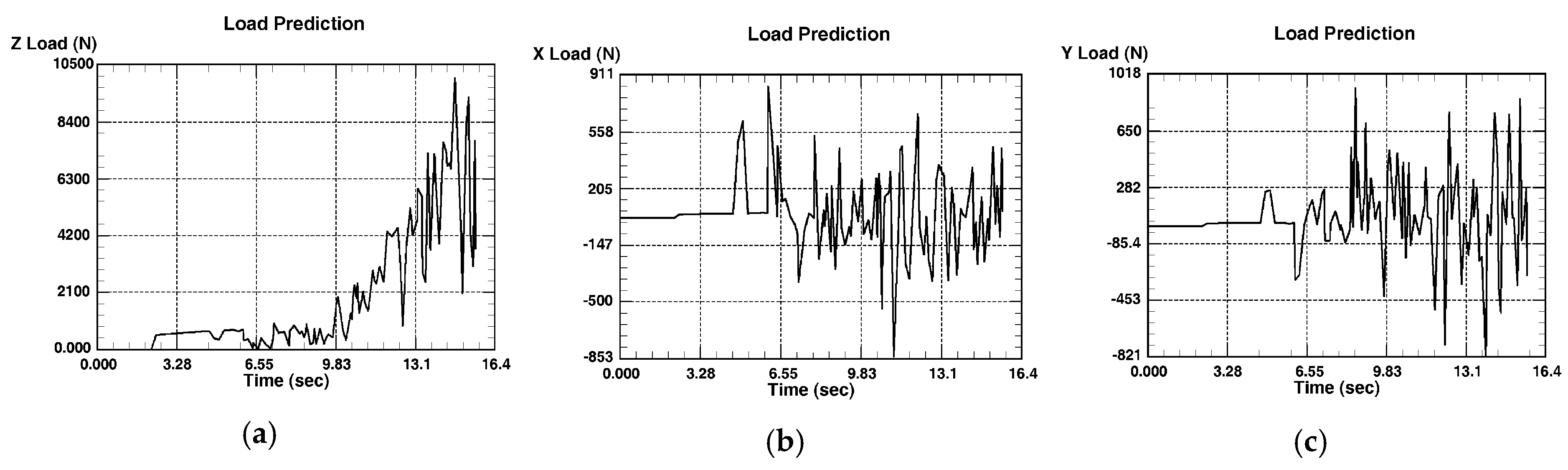
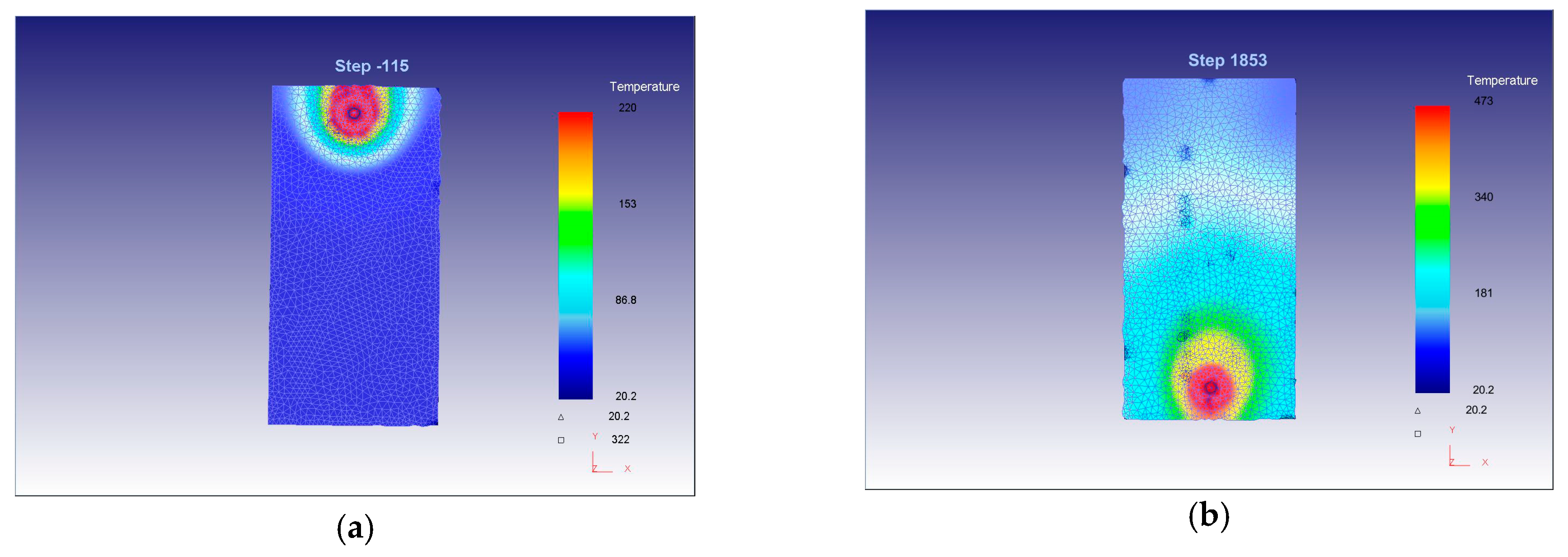
When the simulation starts the numerical calculations for the value of progressing step DSMAX = 0.1 mm are performed, which was previously adopted. Every tenth step is stored in the database. When the finite element mesh parameters reach critical values the automatic remeshing occurs. The process of the first phase ends with the 115-step. Forces
Fz,
Fx, and
Fy which occur during the first phase of the numerical simulations for the 34th point of the experimental plan are presented in
Figure 9.
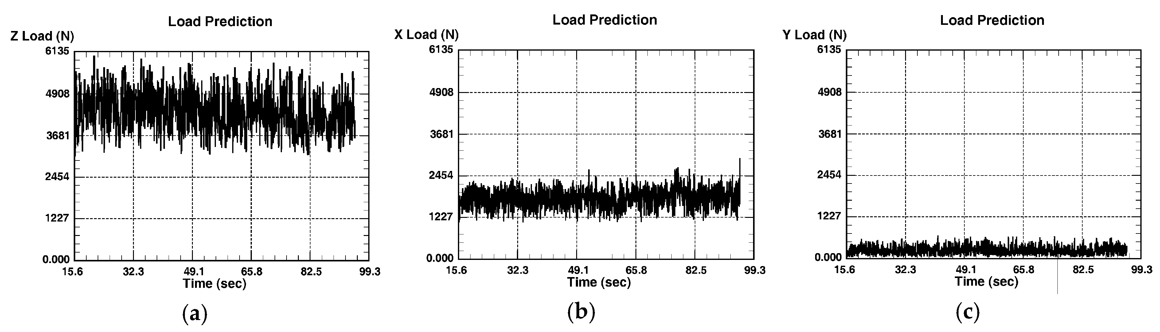
After the commencement of the simulation for the second phase, numerical calculations of the progressing steps are carried out. At this phase, automatic remeshing also takes place. The process was completed in 1853rd step and thus the numerical simulation of FSW. Forces
Fz,
Fx, and
Fy of the second phase of simulation for the 34th point of the experimental plan are given in
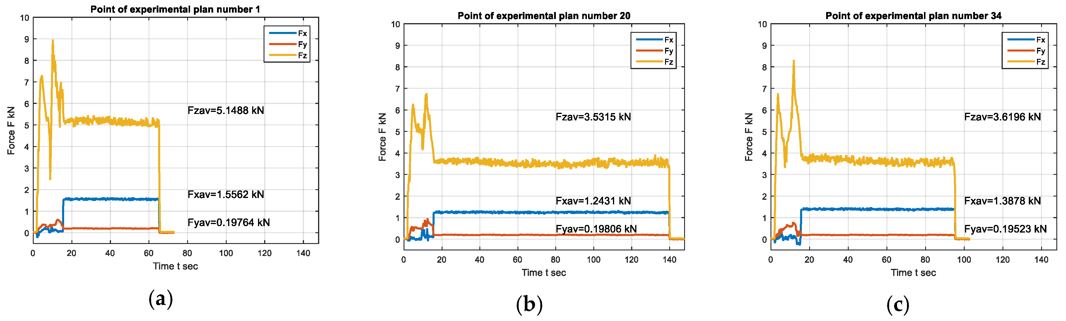
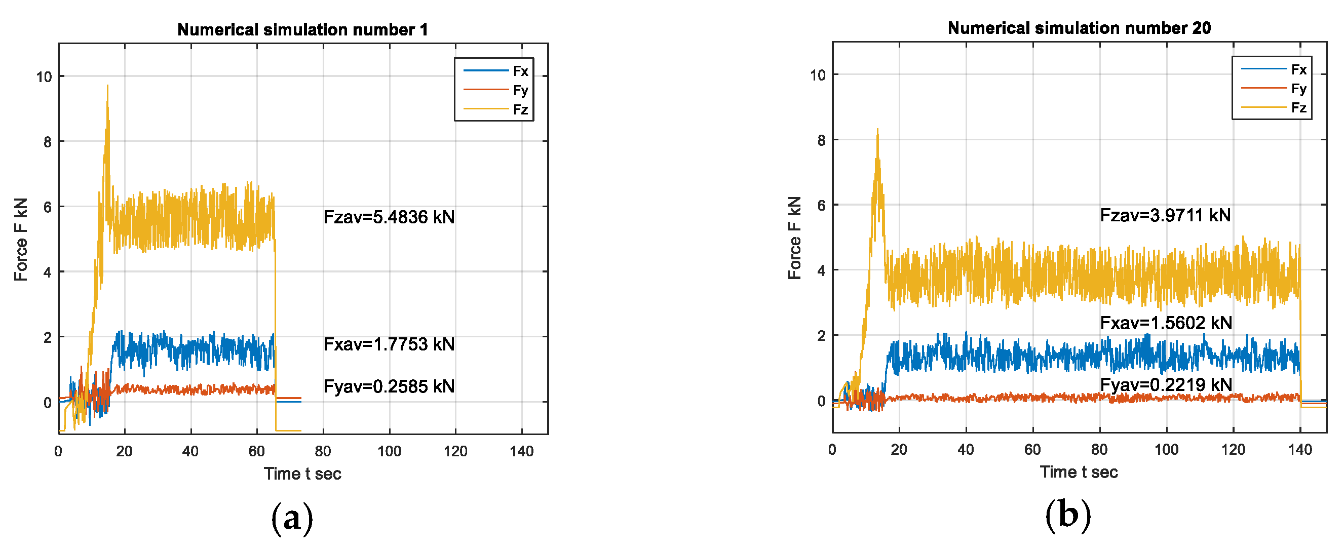
Figure 10. Data for welding force components obtained in DEFORM 3D, for all points of the experimental plan, are processed in the MATLAB (vR2015a, MathWorks, Natick, MA, USA) software, and for the points 1 and 20 of the experimental plan, shown in
Figure 11.
Also, the final distribution of temperature fields at the end of the first (115 steps) and the second phase (1853 step) of the FSW process for the 1st point of the experimental plan is shown in
Figure 12.
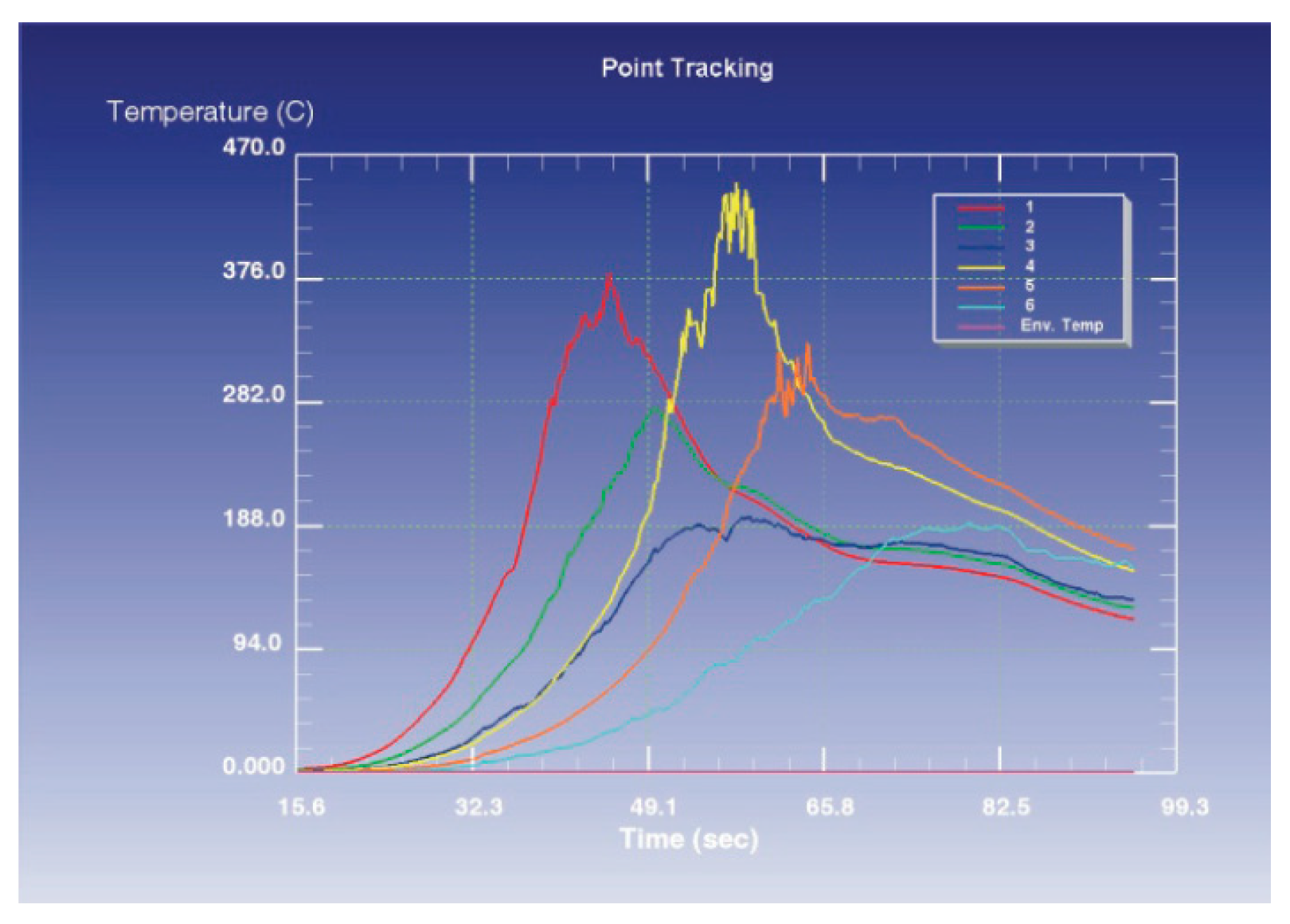
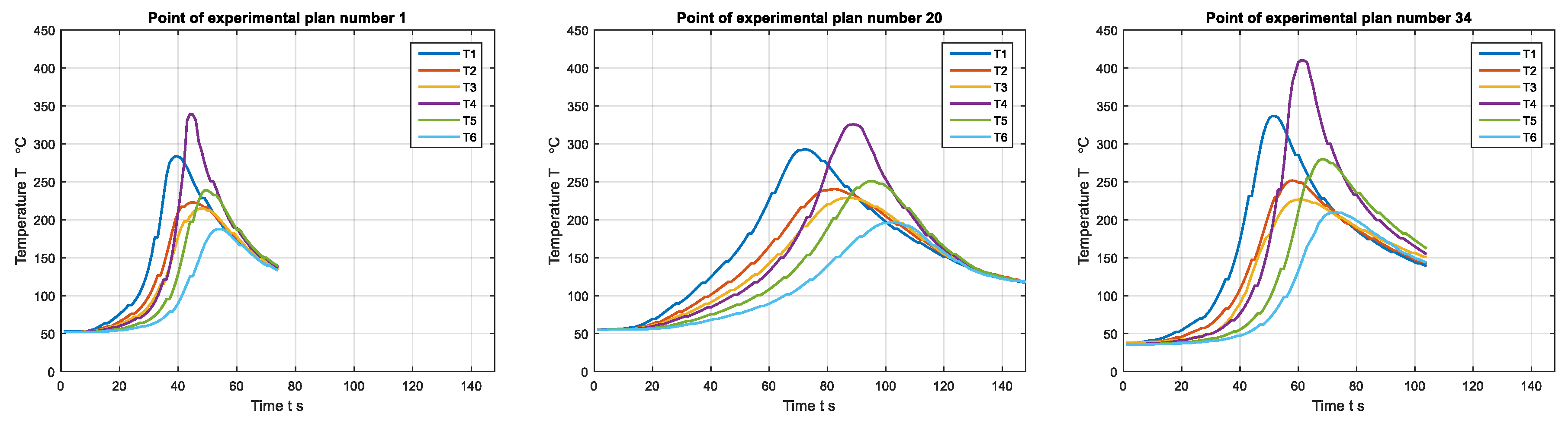
For the defined measurement positions of the workpiece temperature in the microstructural zones in the Point Tracking submodule, the results for the central points of the experimental plan are shown in
Figure 13, while
Table 3 shows the maximum values of the received temperature values in the adopted measuring points for 1 and 20 and 34 the point of the experimental plan [
22].
4. Results and Discussion
During experimental research and numerical simulations, the diagrams of the force components, which occur during the welding process and the temperature diagrams in the adopted measuring positions, are obtained.
From
Figure 4, it can be seen that the duration of the process depends on the welding speed. For the speed of 200 mm/min (
Figure 4a), the duration of the welding process is 49.8 s. For a speed of 80 mm/min (
Figure 4b), the duration of the welding process is 124.5 s. For the center points of the experimental plan and the speed of 125 mm/min (
Figure 4c), the duration of the welding process is 79.68 s. The duration of the process is very important from the point of view of the quality of seams and the productivity of the welding process.
For all points of the experimental plan in the first stage of the process, the forces Fz and Fy reach their highest values. Since in this stage the tool is plunged into the material, variable values of the force are obtained. As Fz is an axial force that presses material, it always has positive values. Due to the consequence of heat generation when plunging the tool, the Fx force material may also have negative values ranging from −0.12 to −0.48 kN for all points of the experimental plan. As the direction of rotation of the tool corresponds to the direction of rotation of the hands on the clock, the values of force Fy are obtained positively, because, during rotation, the tool tends to turn the workpieces in the same direction. At this stage, the maximum values of the force Fz for all points of the experimental plan range from 5.3620 to 9.7300 kN, while the values of force Fy range from 0.3877 to 1.1375 kN.
When the welding process begins, or the second phase, the forces Fx, Fy and Fz retain constant values. For the process of welding by FSW, from the point of view of energy consumption, the most important is the vertical component of the force Fz, which is often called the welding force. For each point of the experimental plan, the component Fz compared to the other two components of the force Fx and Fy has a higher value. The force Fz ranges from 2.4099 to 5.4799 kN, and the force Fx from 1.0118 to 1.7561 kN, while the force Fy is from 0.0987 to 0.2316 kN.
On the value of the Fx force, the welding speed has the greatest influence. The higher the welding speed, the greater the resistance of the material to the tool, and the higher values of the longitudinal force Fx are obtained. Another significant factor that influences the value of force Fx is the angular rotation speed of the tool, and the third surface of the tool in contact with the material. If the rotation speed of tool is larger and the surface of the tool is larger, more heat is generated, so the tool moves easily through the material so that the resistance is smaller and the lower value of the Fx force is obtained. If the rotation speed of tool is smaller, and the surface of the tool will generate less heat, so the resistance to the movement of the tool will be higher, and therefore the longitudinal force Fx will be higher.
During the FSW process, the Fy force acting in the side direction has relatively low values compared to other forces, so its influence on the welding process is relatively small.
In executed numerical simulations, the duration of the process is analogous to experimental.
For all numerical simulations in the first stage of the process, the forces Fz and Fy reach their highest values. Analogously to the experimental values in this stage, variable values of the force are obtained. For numerical simulations, the force Fz always has positive values, while the forces Fx and Fy have negative values in this stage of plunging the tool into the material. Force Fx and Fy at this stage have approximate values that range within ± 1.2 kN. At this stage, the maximum values of the force Fz for all numerical simulations range from 7.1982 to 11.5214 kN.
In the second phase of the process, the forces Fx, Fy and Fz also retain constant values until the simulation is complete, after 166 mm of travel. In each numerical simulation, the component Fz has higher values than the components Fx and Fy. Force Fz in this stage for all numerical simulations ranges from 3.3429 to 6.3681 kN, and force Fx from 1.2968 to 2.2801 kN, while force Fy is from 0.1420 to 0.3103 kN. For numerical simulations of the FSW process, the force Fy, which acts in the side direction, also has relatively small values, so its effect on the friction welding process is small.
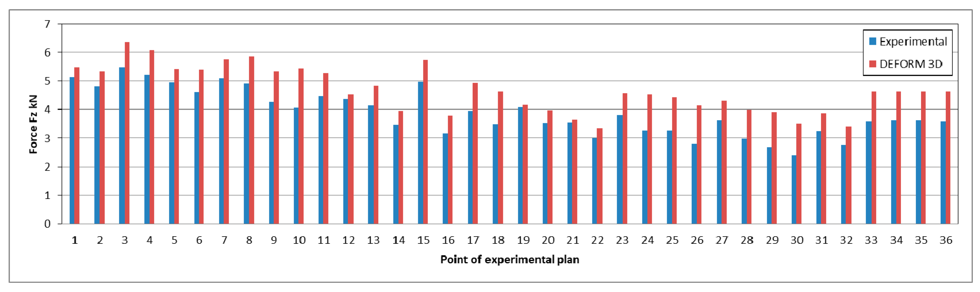
In
Figure 14, the values of the most influential axial force
Fz, that is, the welding forces obtained by experimental and numerical simulations, are given.
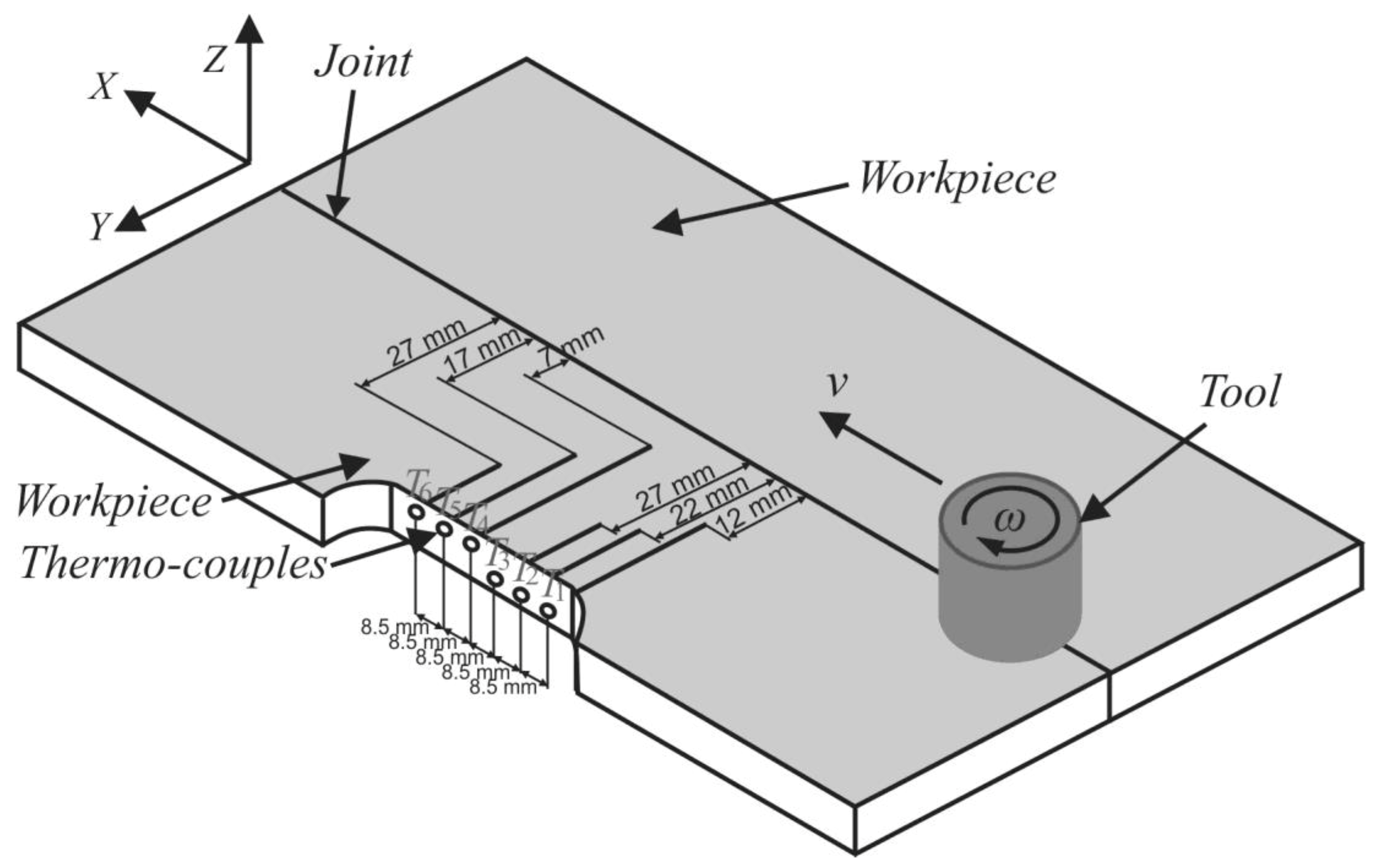
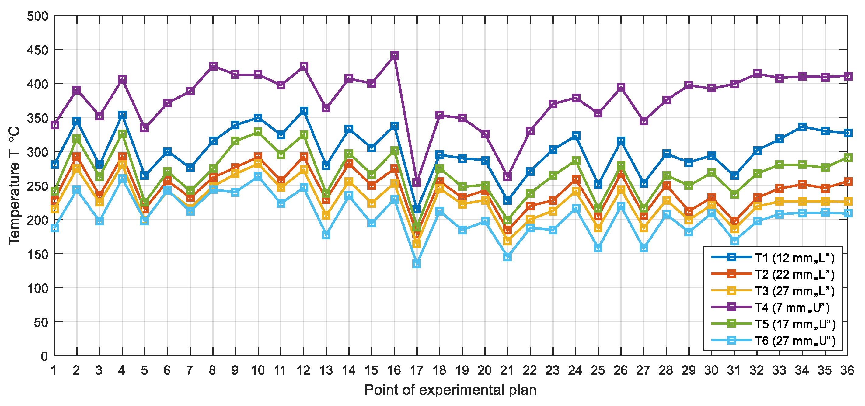
For the analysis of the temperature variation in relation to the variable parameters of experimental research, in
Figure 15, the maximum values of the temperatures measured using thermocouples
T1,
T2,
T3,
T4,
T5, and
T6 for all points of the experimental plan are shown.
The largest measured value of the temperature is at the 16th point of the experimental plan and is 440.4 °C. As the temperature of melted aluminum alloys 6080-T6, 555 °C, it can be noted that the FSW process is performed for all points of the experimental plan in the solid state without the melting effect of the material that characterizes the conventional welding processes. Since temperature is measured at certain distances from the joint line, obtained results can be analyzed. The thermocouple closest to the source of heat is T4. This thermocouple is at a distance from the joint line of 7 mm, so at this measuring point, the highest values of the measured temperature are obtained. The smallest measured value in the thermocouple number T4 is at the 17th point of the experimental plan and is 254.5 °C. Otherwise, in the 17th point of the experimental plan, the least measured values for all other thermocouple positions were obtained, and the smallest was 135.1 °C, at a distance of 27 mm from the joint line in the upper zone. The reason for this low value of the temperature obtained is the consequence of the unfavorable relationship of the varied factors, which resulted in poor quality seams.
At a distance of 12 mm from the joint line in the lower zone, the highest temperature value in the 12th point of the experimental plan is measured and it is 360 °C. At the 10th point of the experimental plan, at a distance of 17 mm from the joint line in the upper zone, the maximum temperature value was measured and it is 328 °C. At this point, the maximum value of the temperature was measured at a distance of 27 mm in the lower zone 281.8 °C and in the upper zone 263 °C. At the 4th point of the experimental plan at a distance of 22 mm from the joint line in the lower zone, the highest temperature value was measured at 292.7 °C.
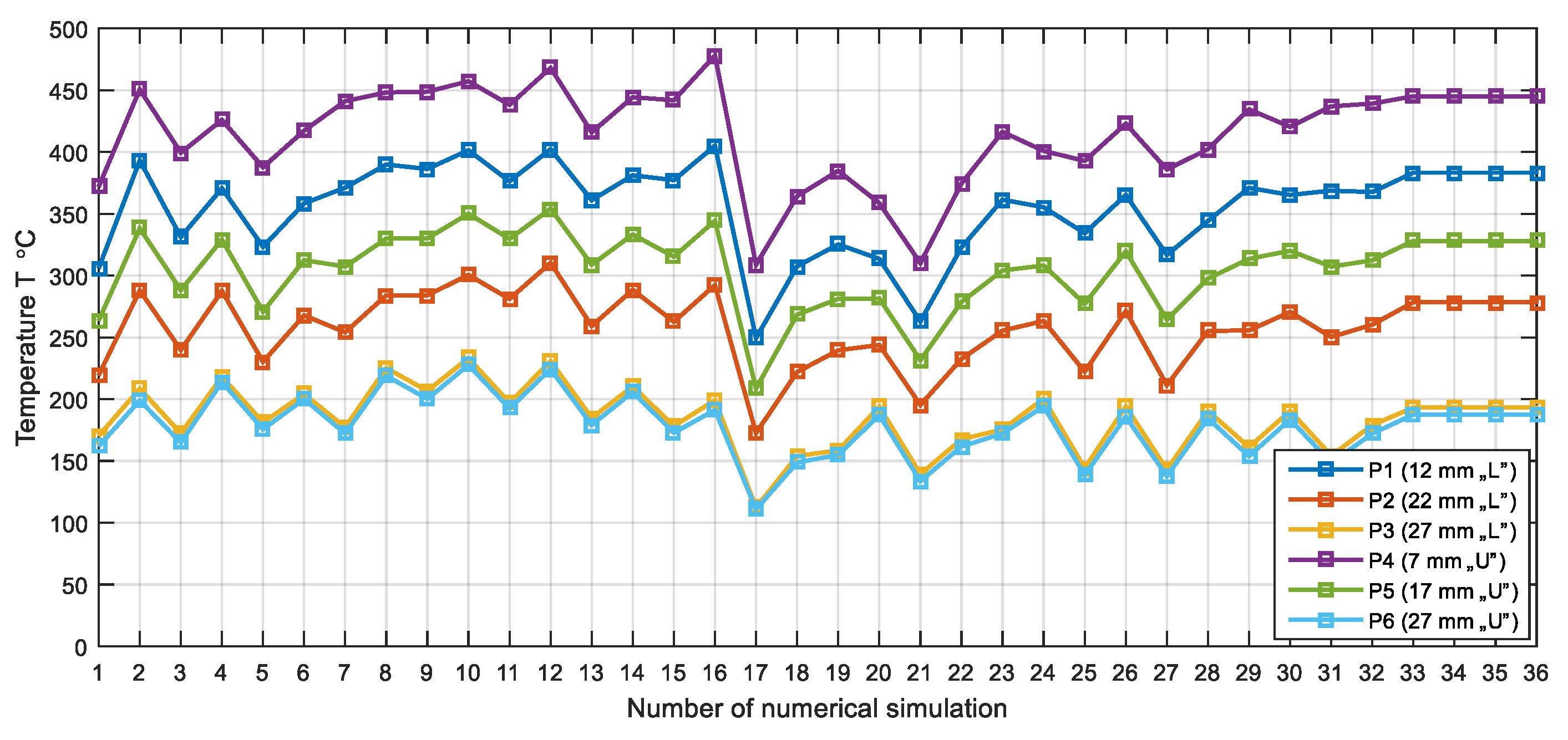
In
Figure 16, a diagram of the maximum received temperature is given in the selected six measurement positions of Point Tracking submodules obtained in the DEFORM 3D software, which are processed in MATLAB, for all numerical simulations performed.
Since point P4 is closest to the joint line, at this point we have the highest values of the numerically generated temperature. The lowest value of the temperature at point P4 is in the 21st simulation and is 310.14 °C. At point P1 located in the lower zone and 12 mm from the joint line, the highest temperature value was obtained also in the 16th simulation, which is 405.04 °C. In the 17th simulation for the points P1, P2, P3, P5, and P6, the lowest temperature values were obtained, and the smallest is at the point P3 of the upper zone, at a distance of 27 mm from the joint line and is 112.30 °C. Point P5 is located in the upper zone at a distance of 17 mm from the joint line, and the highest temperature was measured in the 12th numerical simulation and is 354.15 °C. In the 12th simulation at point P2, located in the lower zone at a distance of 22 mm from the joint line, the highest temperature value was obtained, which is 310.26 °C. In the 10th simulation, at points P3 and P6, the highest temperature was obtained. For point P3 it is 233.26 °C, and for P6, 227.70 °C.
5. Conclusions
In this paper, the force components Fx, Fy and Fz were determined, as well as the distribution of the welded sample temperature from the aluminum alloy obtained by the FSW method. The influence of tool geometry (diameter of the shoulder, pin diameter, and angle of pin slope) and the welding speed and rotation speed on the change of force and temperature were investigated. The experiments were performed experimentally using special tools and accessories, as well as numerically, using the DEFORM 3D software package. By analyzing the obtained dependencies, we conclude that the FSW technology can be successfully applied to the welding of the investigated alumina alloy AA6082-T6.
A special contribution of the paper is the comparison of experimental and numerical results in the case of simultaneous changes in geometric and kinematic parameters, which is enabled by the adopted experimental plan.
For the FSW welding process from the investigated components of the force, the most important is the axial component Fz, which is often called the welding force. It can be concluded that the geometric parameters of the tool, especially the size of the shoulder of the tool, have the largest influence on the Fz value. All obtained values of the Fz force can be divided into three areas. The first 16 points of the experimental plan belong to the first area. This is the area where the diameter of the shoulder of the tool is 28 mm. Here the values of the force Fz are obtained from the limits of 3.4614 to 5.4799 kN. The other area belongs to the points of the experimental plan from 17 to 32, where the diameter of the shoulder of the tool is 25 mm, and the force ranges from 2.4099 to 4.0428 kN. The third area belongs to the central points of the plan, where the diameter of the shoulder of the tool is 26.46 mm, and the mean value of the force Fz at these points is 3.6008 kN.
In numerical simulations, all the obtained values of the force Fz can also be divided into three areas: The area of the larger diameter of the shoulder of the tool of 28 mm, the area of the smaller diameter of the shoulder of the tool of 25 mm and the area of 26.46 mm (center point of the plan).
Welding forces obtained by numerical simulation are approximately 10% higher than experimental forces, which means that the FSW process can be successfully simulated with FEM.
We can conclude that the largest maximum experimental measured values of the temperature are obtained in the first 16 points of the experimental plan where the dominant factor is the diameter of the shoulder of the tool of 28 mm. In the central points of the experimental plan where the diameter of the shoulder is 26.46 mm, small temperature values are obtained, where the average temperature at a distance of 7 mm from the joint line is 409.6 °C, and at a distance of 27 mm, 209.1 °C in the upper zone. In the points of the experimental plan from 17 to 32, where the smaller diameter of the tool 25 mm, a significantly lower temperature value is obtained.
The numerical simulations also distinguish three temperature regions in which the temperature values are analogous to the experimental results.
A comparison of experimentally obtained temperature values with the values obtained by numerical simulation shows a relatively good agreement with the difference below 10%. This allows the conclusion that heat generation and temperature distribution within the workpiece in the FSW process can be successfully simulated by FEM.
The deviation of numerical results from a physical experiment is conditioned by the DEFORM-3D characteristics. The software is based on the theory of small elasto-plastic deformations that, through a large number of steps, describe the large deformations that characterize the FSW process. High non-linearity is conditioned by the frequent occurrence of remeshing, i.e., transferring data from the old deformed mesh to a new undeformed mesh, which makes engineering tolerances of 10% possible.
Because of the complexity of the FSW process, which is accompanied by a large number of influencing parameters, this technology is a very wide research area. In this sense, our further research will focus on further theoretical analysis, experimental verification and numerical simulation of the FSW process, i.e., TES approach (T—Theory, E—Experiment, and S—Simulation).


