Texture-Based Metallurgical Phase Identification in Structural Steels: A Supervised Machine Learning Approach


Abstract
:1. Introduction
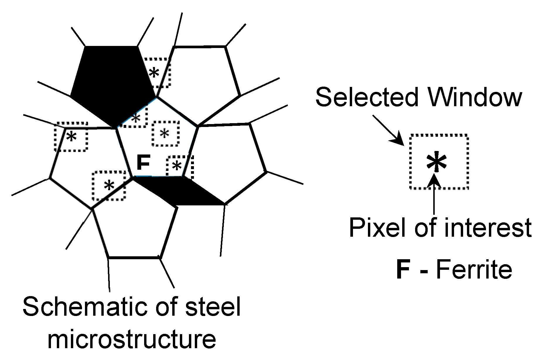
2. Texture
Gray Level Co-occurrence Matrix (GLCM) and Textural Features
3. Supervised Machine Learning
3.1. Naïve Bayes
3.2. K-Nearest Neighbor
3.3. Linear Discriminant Analysis
3.4. Decision Tree
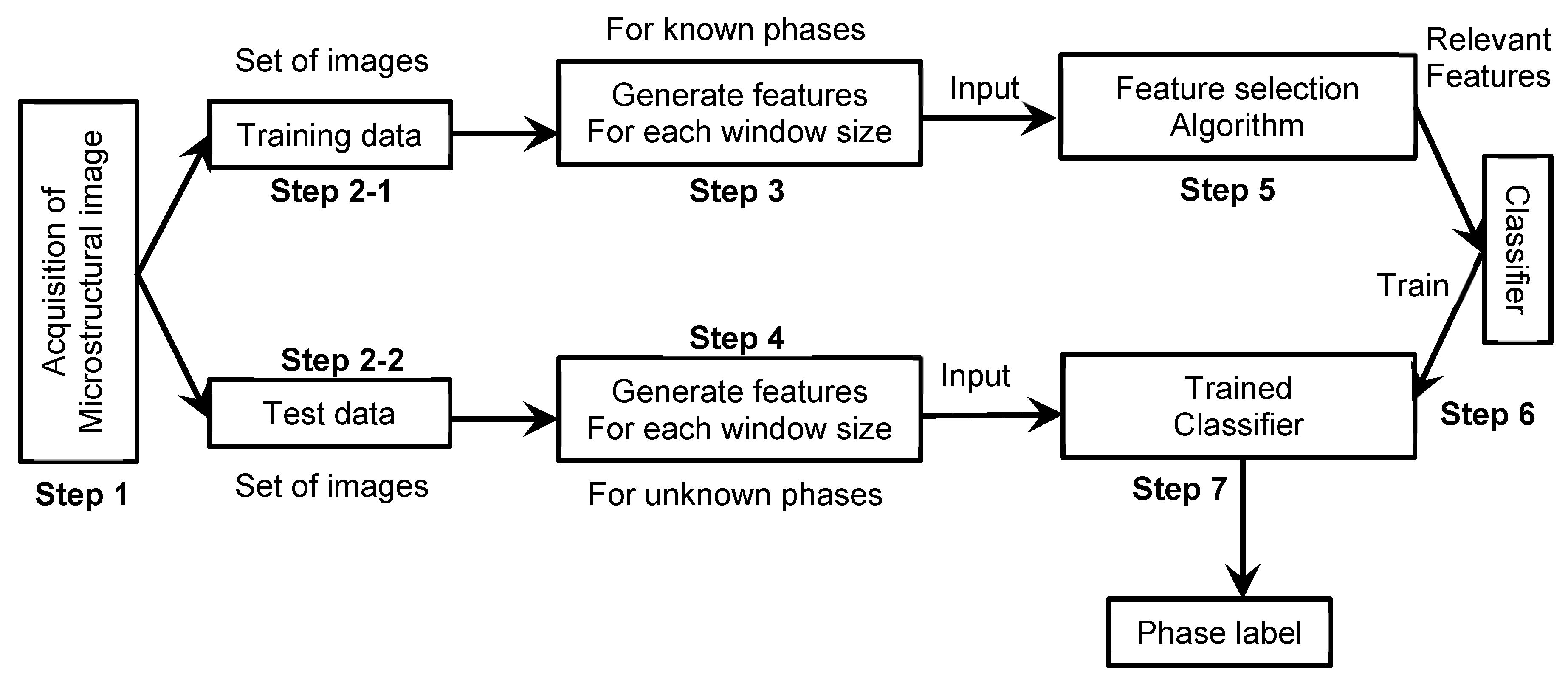
4. Methodology
5. Feature Selection
5.1. Feature Ranking
5.2. Selection of the Feature Subset
5.3. Performance Assessment of the Classifier
6. Results
6.1. Feature Ranking
6.2. Feature Subset Selection
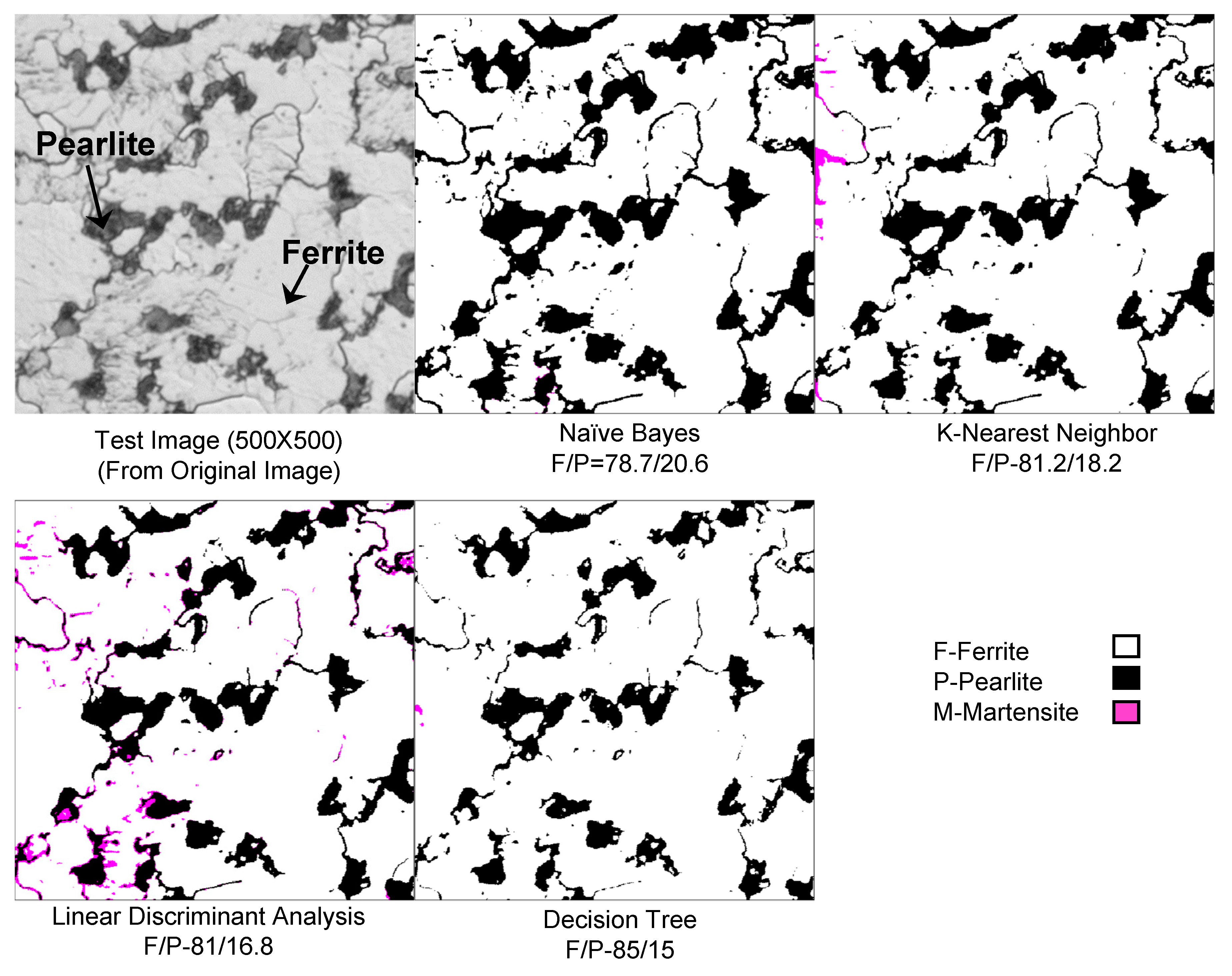
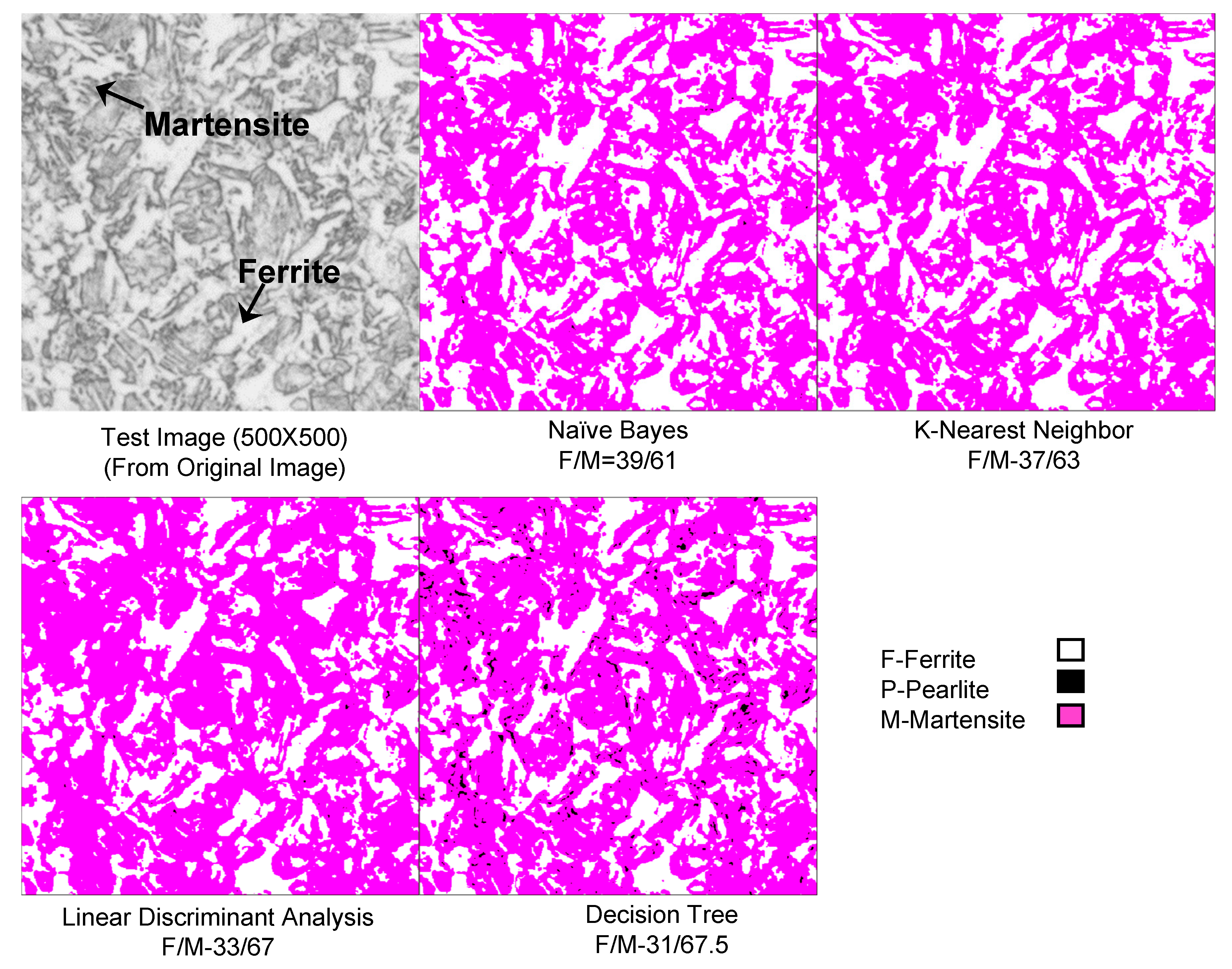
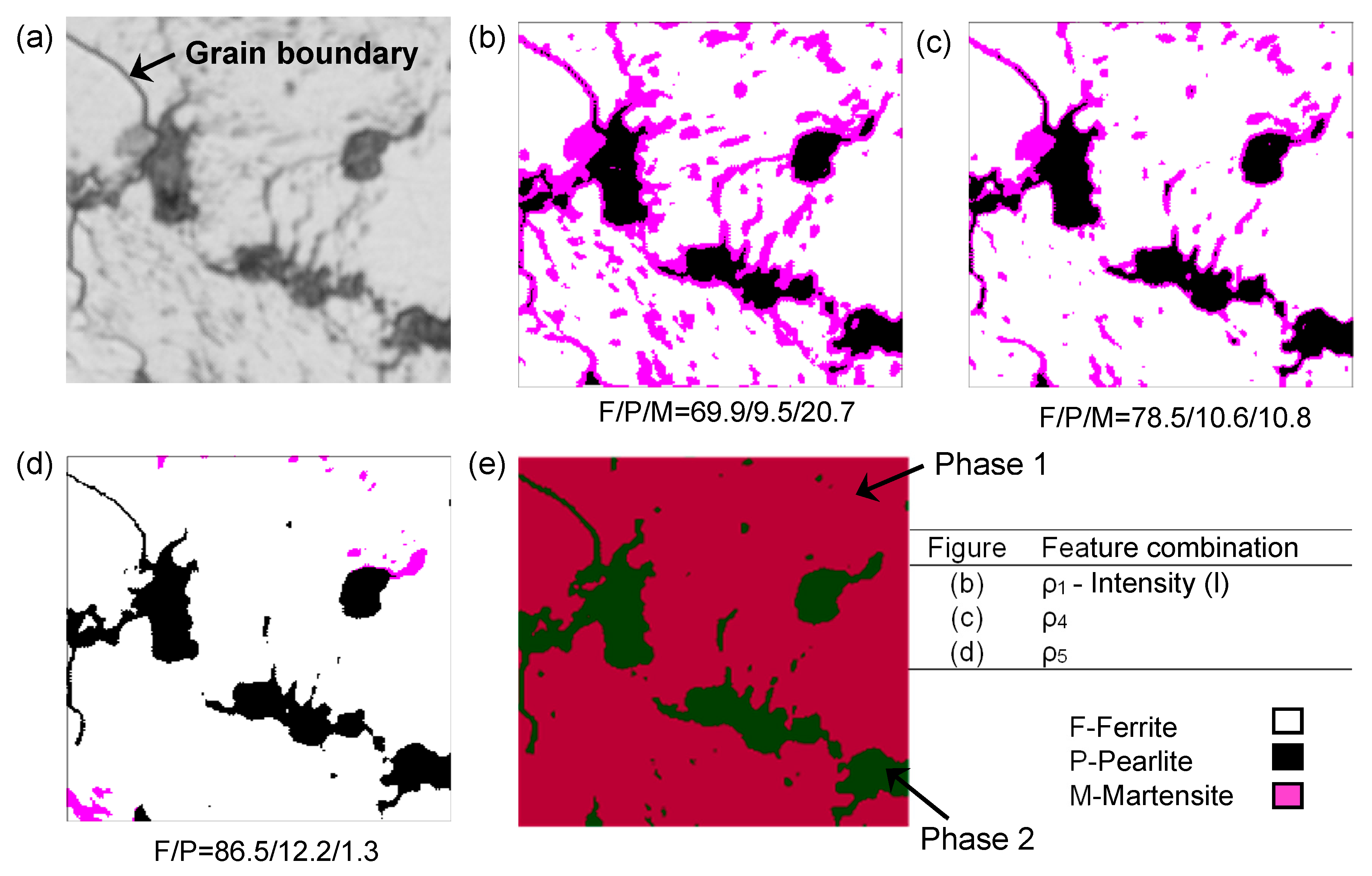
6.3. Example Problem
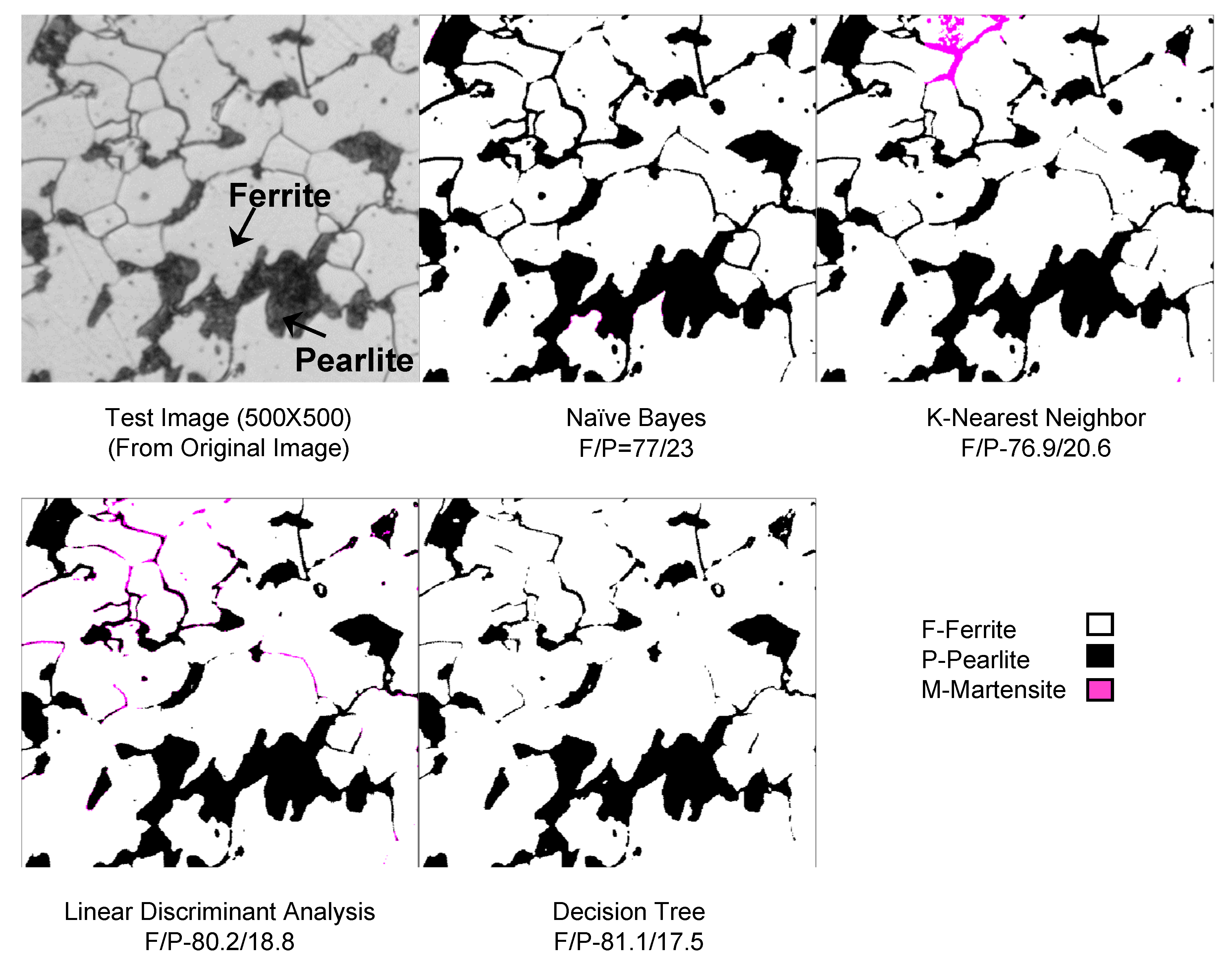
6.4. Validation
7. Summary and Recommendations
Author Contributions
Funding
Acknowledgments
Conflicts of Interest
References
- Clemens, H.; Mayer, S.; Scheu, C. Microstructure and Properties of Engineering Materials. In Neutrons and Synchrotron Radiation in Engineering Materials Science: From Fundamentals to Applications; Wiley: Hoboken, NJ, USA, 2017; pp. 1–20. [Google Scholar]
- Fan, Z. Microstructure and Mechanical Properties of Multiphase Materials. Ph.D. Thesis, University of Surrey, Guildford, UK, February 1993. [Google Scholar]
- Bales, B.; Pollock, T.; Petzold, L. Segmentation-free image processing and analysis of precipitate shapes in 2D and 3D. Modell. Simul. Mater. Sci. Eng. 2017, 25, 045009. [Google Scholar] [CrossRef]
- Beddoes, J.; Bibby, M. Principles of Metal Manufacturing Processes; Butterworth-Heinemann: Oxford, UK, 1999. [Google Scholar]
- Hall, E. The deformation and ageing of mild steel: III discussion of results. Proc. Phys. Soc. Sect. B 1951, 64, 747. [Google Scholar] [CrossRef]
- Petch, N. The influence of grain boundary carbide and grain size on the cleavage strength and impact transition temperature of steel. Acta Metall. 1986, 34, 1387–1393. [Google Scholar] [CrossRef]
- American Society for Testing and Materials. ASTM E112-96 (2004) e2: Standard Test Methods for Determining Average Grain Size; ASTM: West Conshohocken, PA, USA, 2004. [Google Scholar]
- ASTM E562-08. Standard Test Method for Determining Volume Fraction by Systematic Manual Point Count; ASTM International: West Conshohocken, PA, USA, 2008. [Google Scholar]
- Campbell, A.; Murray, P.; Yakushina, E.; Marshall, S.; Ion, W. New methods for automatic quantification of microstructural features using digital image processing. Mater. Des. 2018, 141, 395–406. [Google Scholar] [CrossRef]
- Ayech, M.B.H.; Amiri, H. Texture description using statistical feature extraction. In Proceedings of the 2016 2nd International Conference on Advanced Technologies for Signal and Image Processing (ATSIP), Monastir, Tunisia, 21–23 March 2016; IEEE: Piscataway Township, NJ, USA, 2016; pp. 223–227. [Google Scholar]
- Acharya, T.; Ray, A.K. Image Processing: Principles and Applications; John Wiley & Sons: Hoboken, NJ, USA, 2005. [Google Scholar]
- Pakhira Malay, K. Digital Image Processing and Pattern Recognition; PHI Learning Private Limited: Delhi, India, 2011. [Google Scholar]
- Sobel, I. Camera Models and Machine Perception; Computer Science Department, Technion: Haifa, Israel, 1972. [Google Scholar]
- Dougherty, G. Digital Image Processing for Medical Applications; Cambridge University Press: Cambridge, UK, 2009. [Google Scholar]
- Jahne, B. Digital Image Processing: Concepts, Algorithms, and Scientific Aplications; Springer-Verlag: Heildelberg/Berlin, Germany, 1997; p. 570. [Google Scholar]
- Otsu, N. A threshold selection method from gray-level histograms. IEEE Trans. Syst. Man Cybern. 1979, 9, 62–66. [Google Scholar] [CrossRef]
- Jain, A.K. Fundamentals of Digital Image Processing; Englewood Cliffs, N.J., Prentice Hall: Upper Saddle River, NJ, USA, 1989. [Google Scholar]
- Jiang, X.; Zhang, R.; Nie, S. Image segmentation based on level set method. Phys. Procedia 2012, 33, 840–845. [Google Scholar] [CrossRef]
- Sosa, J.M.; Huber, D.E.; Welk, B.; Fraser, H.L. Development and application of MIPAR™: A novel software package for two-and three-dimensional microstructural characterization. Integrating Mater. Manuf. Innov. 2014, 3, 10. [Google Scholar] [CrossRef]
- Bonnet, N. Some trends in microscope image processing. Micron 2004, 35, 635–653. [Google Scholar] [CrossRef]
- Yang, D.; Liu, Z. Quantification of microstructural features and prediction of mechanical properties of a dual-phase Ti-6Al-4V alloy. Materials 2016, 9, 628. [Google Scholar] [CrossRef] [PubMed]
- Buriková, K.; Rosenberg, G. Quantification of microstructural parameter ferritic-martensite dual phase steel by image analysis. Metal 2009, 5, 19–21. [Google Scholar]
- Ontman, A.Y.; Shiflet, G.J. Microstructure segmentation using active contours—Possibilities and limitations. JOM 2011, 63, 44–48. [Google Scholar] [CrossRef]
- Coverdale, G.; Chantrell, R.; Martin, G.; Bradbury, A.; Hart, A.; Parker, D. Cluster analysis of the microstructure of colloidal dispersions using the maximum entropy technique. J. Magn. Magn. Mater. 1998, 188, 41–51. [Google Scholar] [CrossRef]
- Azimi, S.M.; Britz, D.; Engstler, M.; Fritz, M.; Mücklich, F. Advanced Steel Microstructural Classification by Deep Learning Methods. Sci. Rep. 2018, 8, 2128. [Google Scholar] [CrossRef]
- Prakash, P.; Mytri, V.; Hiremath, P. Fuzzy Rule Based Classification and Quantification of Graphite Inclusions from Microstructure Images of Cast Iron. Microsc. Microanal. 2011, 17, 896–902. [Google Scholar] [CrossRef]
- DeCost, B.L.; Holm, E.A. A computer vision approach for automated analysis and classification of microstructural image data. Comput. Mater. Sci. 2015, 110, 126–133. [Google Scholar] [CrossRef]
- Haralick, R.M. Statistical and structural approaches to texture. Proc. IEEE 1979, 67, 786–804. [Google Scholar] [CrossRef]
- Haralick, R.M.; Shanmugam, K. Textural features for image classification. IEEE Trans. Syst. Man Cybern. 1973, 6, 610–621. [Google Scholar] [CrossRef]
- Soh, L.-K.; Tsatsoulis, C. Texture analysis of SAR sea ice imagery using gray level co-occurrence matrices. IEEE Trans. Geosci. Remote Sens. 1999, 37, 780–795. [Google Scholar] [CrossRef]
- Gómez, W.; Pereira, W.; Infantosi, A.F.C. Analysis of co-occurrence texture statistics as a function of gray-level quantization for classifying breast ultrasound. IEEE Trans. Med. Imaging 2012, 31, 1889–1899. [Google Scholar] [CrossRef] [PubMed]
- Camastra, F.; Vinciarelli, A. Machine Learning for Audio, Image and Video Analysis: Theory and Applications; Springer-Verlag: London, UK, 2015. [Google Scholar]
- Sessions, V.; Valtorta, M. The Effects of Data Quality on Machine Learning Algorithms. ICIQ 2006, 6, 485–498. [Google Scholar]
- James, G.; Witten, D.; Hastie, T.; Tibshirani, R. An Introduction to Statistical Learning; Springer-Verlag: New York, NY, USA, 2013; Volume 112. [Google Scholar]
- Kelleher, J.D.; Mac Namee, B.; D’Arcy, A. Fundamentals of Machine Learning for Predictive Data Analytics: Algorithms, Worked Examples, and Case Studies; MIT Press: Cambridge, MA, USA, USA 2015. [Google Scholar]
- Aggarwal, C.C. Data Classification: Algorithms and Applications; CRC Press: New York, NY, USA, 2014. [Google Scholar]
- Naik, D.L.; Kiran, R. Naïve Bayes classifier, multivariate linear regression and experimental testing for classification and characterization of wheat straw based on mechanical properties. Ind. Crops Prod. 2018, 112, 434–448. [Google Scholar] [CrossRef]
- Kononenko, I.; Kukar, M. Machine Learning and Data Mining; Horwood Publishing: West Sussex, UK, 2007. [Google Scholar]
- Mitchell, T.M. Machine Learning; McGraw-Hill, Inc.: New York, NY, USA, 1997; p. 432. [Google Scholar]
- Quinlan, J.R. C4.5: Programs for Machine Learning; Morgan Kaufmann Publishers: San Mateo, CA, USA, 2014. [Google Scholar]
- Bramer, M. Principles of Data Mining; Springer-Verlag: London, UK, 2007; Volume 180. [Google Scholar]
- Sajid, H.U.; Kiran, R. Influence of stress concentration and cooling methods on post-fire mechanical behavior of ASTM A36 steels. Constr. Build. Mater. 2018, 186, 920–945. [Google Scholar] [CrossRef]
- Sajid, H.U.; Kiran, R. Post-fire mechanical behavior of ASTM A572 steels subjected to high stress triaxialities. Eng. Struct. 2019, 191, 323–342. [Google Scholar] [CrossRef]
- Kira, K.; Rendell, L.A. The feature selection problem: Traditional methods and a new algorithm. In Proceedings of the Tenth National Conference on Artificial Intelligence, San Jose, CA, USA, 12–16 July 1992; pp. 129–134. [Google Scholar]
- Urbanowicz, R.J.; Meeker, M.; La Cava, W.; Olson, R.S.; Moore, J.H. Relief-based feature selection: introduction and review. J. Biomed. Inf. 2018. [Google Scholar] [CrossRef]
- Robnik-Šikonja, M.; Kononenko, I. Theoretical and empirical analysis of ReliefF and RReliefF. Mach. Learn. 2003, 53, 23–69. [Google Scholar] [CrossRef]
- Müller, M.E. Relational Knowledge Discovery; Cambridge University Press: Cambridge, UK, 2012. [Google Scholar]
- Akosa, J. Predictive Accuracy: A Misleading Performance Measure for Highly Imbalanced Data. In Proceedings of the SAS Global Forum 2017, Orlando, FL, USA, 2–5 April 2017. [Google Scholar]
- Sokolova, M.; Lapalme, G. A systematic analysis of performance measures for classification tasks. Inf. Process. Manag. 2009, 45, 427–437. [Google Scholar] [CrossRef]
- Ratanamahatana, C.A.; Gunopulos, D. Scaling up the naive Bayesian classifier: Using decision trees for feature selection. 2002. [Google Scholar]
- Kohavi, R.; John, G.H. Wrappers for feature subset selection. Artif. Intel. 1997, 97, 273–324. [Google Scholar] [CrossRef]


| Notation | Texture Feature | Equation |
|---|---|---|
| T1 | Autocorrelation | |
| T2 | Contrast | |
| T3 | Cluster prominence | |
| T4 | Cluster shade | |
| T5 | Dissimilarity | |
| T6 | Energy | |
| T7 | Entropy | |
| T8 | Homogeneity | |
| T9 | Maximum probability | |
| T10 | Sum of squares | |
| T11 | Sum average | |
| T12 | Sum entropy | |
| T13 | Sum variance | |
| T14 | Difference variance | |
| T15 | Difference entropy | |
| T16 | Information measure of correlation I | |
| T17 | Inverse difference normalized | |
| T18 | Inverse difference moment normalized |
| Rank | 61 × 61 | 81 × 81 | 101 × 101 | 121 × 121 | 161 × 161 |
|---|---|---|---|---|---|
| 1 | Intensity | Intensity | Intensity | Intensity | Intensity |
| 2 | Maximum probability | Maximum probability | Maximum probability | Maximum probability | Maximum probability |
| 3 | Auto-correlation | Sum of squares | Sum of squares | Cluster shade | Sum of squares |
| 4 | Sum of squares | Auto-correlation | Auto-correlation | Inverse correlation | Auto-correlation |
| 5 | Entropy | Sum variance | Sum variance | Sum of squares | Cluster shade |
| 6 | Sum variance | Energy | Inverse correlation | Auto-correlation | Sum variance |
| 7 | Cluster shade | Cluster shade | Cluster shade | Energy | Sum average |
| 8 | Sum average | Sum average | Energy | Sum variance | Inverse correlation |
| 9 | Inverse difference moment | Sum entropy | Sum average | Inverse difference normalized | Inverse difference normalized |
| 10 | Sum entropy | Entropy | Inverse difference normalized | Sum average | Energy |
| - | Predicted Class Label | ||||
|---|---|---|---|---|---|
| Actual Class Label | |||||
| Window Size | Combination | |||||
|---|---|---|---|---|---|---|
| ρ1 | ρ2 | ρ3 | ρ4 | ρ5 | ρ6 | |
| 161 × 161 | Intensity | ρ1 + T9 | ρ1 + T10 | ρ2 + T1 | ρ3 + T4 | ρ4 + T13 |
| 121 × 121 | Intensity | ρ1 + T9 | ρ1 + T4 | ρ2 + T16 | ρ3 + T10 | ρ4 + T1 |
| 101 × 101 | Intensity | ρ1 + T9 | ρ1 + T10 | ρ2 + T1 | ρ3 + T13 | ρ4 + T16 |
| 81 × 81 | Intensity | ρ1 + T9 | ρ1 + T10 | ρ2 + T1 | ρ3 + T13 | ρ4 + T6 |
| 61 × 61 | Intensity | ρ1 + T9 | ρ1 + T1 | ρ2 + T10 | ρ3 + T7 | ρ4 + T13 |
| Size | C for ρ2 | Fm | C for ρ3 | Fm | C for ρ4 | Fm | C for ρ5 | Fm | C for ρ6 | Fm | ||||||||||
|---|---|---|---|---|---|---|---|---|---|---|---|---|---|---|---|---|---|---|---|---|
| 161 | 0.976 | 0.000 | 0.024 | 95.22 | 0.992 | 0.000 | 0.008 | 97.70 | 0.968 | 0.016 | 0.016 | 95.62 | 0.810 | 0.016 | 0.175 | 91.55 | 0.849 | 0.016 | 0.135 | 90.32 |
| 0.009 | 0.954 | 0.037 | 0.000 | 1.000 | 0.000 | 0.000 | 0.991 | 0.009 | 0.000 | 1.000 | 0.000 | 0.009 | 0.991 | 0.000 | ||||||
| 0.067 | 0.000 | 0.933 | 0.067 | 0.033 | 0.900 | 0.033 | 0.067 | 0.900 | 0.000 | 0.017 | 0.983 | 0.050 | 0.050 | 0.900 | ||||||
| Acc. | - | 95.91 | - | - | - | 97.62 | - | - | - | 96.26 | - | - | - | 91.50 | - | - | - | 91.16 | - | - |
| 121 | 0.976 | 0.008 | 0.016 | 94.69 | 0.849 | 0.016 | 0.135 | 93.00 | 0.881 | 0.000 | 0.119 | 92.61 | 0.913 | 0.000 | 0.087 | 94.29 | 0.929 | 0.008 | 0.063 | 95.79 |
| 0.000 | 0.991 | 0.009 | 0.000 | 1.000 | 0.000 | 0.009 | 0.981 | 0.009 | 0.009 | 0.991 | 0.000 | 0.000 | 1.000 | 0.000 | ||||||
| 0.133 | 0.017 | 0.850 | 0.017 | 0.000 | 0.983 | 0.033 | 0.017 | 0.950 | 0.050 | 0.000 | 0.950 | 0.033 | 0.000 | 0.967 | ||||||
| Acc. | - | 95.58 | - | - | - | 93.19 | - | - | - | 93.19 | - | - | - | 94.89 | - | - | - | 96.26 | - | - |
| 101 | 0.968 | 0.000 | 0.032 | 95.05 | 0.952 | 0.000 | 0.048 | 94.69 | 0.944 | 0.008 | 0.048 | 92.59 | 0.913 | 0.000 | 0.087 | 94.10 | 0.944 | 0.000 | 0.056 | 95.99 |
| 0.000 | 0.972 | 0.028 | 0.000 | 0.981 | 0.019 | 0.000 | 0.991 | 0.009 | 0.000 | 1.000 | 0.000 | 0.000 | 1.000 | 0.000 | ||||||
| 0.067 | 0.017 | 0.917 | 0.067 | 0.017 | 0.917 | 0.133 | 0.033 | 0.833 | 0.033 | 0.033 | 0.933 | 0.033 | 0.017 | 0.950 | ||||||
| Acc. | - | 95.92 | - | - | - | 95.60 | - | - | - | 93.88 | - | - | - | 94.89 | - | - | - | 96.59 | - | - |
| 81 | 0.960 | 0.000 | 0.040 | 95.18 | 0.968 | 0.000 | 0.032 | 94.99 | 0.952 | 0.008 | 0.040 | 94.71 | 0.881 | 0.008 | 0.111 | 90.24 | 0.849 | 0.000 | 0.151 | 91.21 |
| 0.000 | 0.963 | 0.037 | 0.000 | 0.981 | 0.019 | 0.000 | 1.000 | 0.000 | 0.000 | 0.981 | 0.019 | 0.000 | 0.991 | 0.009 | ||||||
| 0.033 | 0.017 | 0.950 | 0.067 | 0.033 | 0.900 | 0.083 | 0.033 | 0.883 | 0.100 | 0.033 | 0.867 | 0.017 | 0.050 | 0.933 | ||||||
| Acc. | - | 95.92 | - | - | - | 95.92 | - | - | - | 95.58 | - | - | - | 91.49 | - | - | - | 91.84 | - | - |
| 61 | 0.984 | 0.000 | 0.016 | 94.09 | 0.952 | 0.000 | 0.048 | 93.85 | 0.921 | 0.000 | 0.079 | 92.61 | 0.865 | 0.000 | 0.135 | 92.46 | 0.889 | 0.000 | 0.111 | 92.75 |
| 0.000 | 0.963 | 0.037 | 0.000 | 0.981 | 0.019 | 0.000 | 1.000 | 0.000 | 0.000 | 0.981 | 0.019 | 0.000 | 0.991 | 0.009 | ||||||
| 0.100 | 0.033 | 0.867 | 0.117 | 0.000 | 0.883 | 0.017 | 0.117 | 0.867 | 0.033 | 0.000 | 0.967 | 0.017 | 0.050 | 0.933 | ||||||
| Acc. | - | 95.24 | - | - | - | 94.89 | - | - | - | 93.88 | - | - | - | 92.86 | - | - | - | 93.54 | - | - |
| Size | C for ρ2 | Fm | C for ρ3 | Fm | C for ρ4 | Fm | C for ρ5 | Fm | C for ρ6 | Fm | ||||||||||
|---|---|---|---|---|---|---|---|---|---|---|---|---|---|---|---|---|---|---|---|---|
| 161 | 0.944 | 0.000 | 0.056 | 91.05 | 0.968 | 0.000 | 0.032 | 93.83 | 0.976 | 0.000 | 0.024 | 94.57 | 0.992 | 0.000 | 0.008 | 97.23 | 0.960 | 0.000 | 0.040 | 94.71 |
| 0.000 | 0.944 | 0.056 | 0.000 | 0.954 | 0.046 | 0.000 | 0.972 | 0.028 | 0.009 | 0.981 | 0.009 | 0.000 | 0.972 | 0.028 | ||||||
| 0.133 | 0.017 | 0.850 | 0.083 | 0.017 | 0.900 | 0.100 | 0.017 | 0.883 | 0.067 | 0.000 | 0.933 | 0.083 | 0.000 | 0.917 | ||||||
| Acc. | - | 92.52 | - | - | - | 94.89 | - | - | - | 95.58 | - | - | - | 97.62 | - | - | - | 95.58 | - | - |
| 121 | 0.968 | 0.000 | 0.032 | 93.35 | 0.968 | 0.000 | 0.032 | 94.21 | 0.984 | 0.000 | 0.016 | 93.79 | 0.960 | 0.000 | 0.040 | 94.36 | 0.968 | 0.000 | 0.032 | 92.95 |
| 0.000 | 0.972 | 0.028 | 0.000 | 0.972 | 0.028 | 0.000 | 0.944 | 0.056 | 0.009 | 0.981 | 0.009 | 0.000 | 0.963 | 0.037 | ||||||
| 0.150 | 0.000 | 0.850 | 0.117 | 0.000 | 0.883 | 0.117 | 0.000 | 0.883 | 0.117 | 0.000 | 0.883 | 0.150 | 0.000 | 0.850 | ||||||
| Acc. | - | 94.56 | - | - | - | 95.24 | - | - | - | 94.89 | - | - | - | 95.24 | - | - | - | 94.22 | - | - |
| 101 | 0.944 | 0.000 | 0.056 | 90.94 | 0.968 | 0.000 | 0.032 | 93.78 | 0.976 | 0.000 | 0.024 | 91.18 | 0.952 | 0.000 | 0.048 | 92.31 | 0.976 | 0.000 | 0.024 | 93.75 |
| 0.000 | 0.963 | 0.037 | 0.000 | 0.963 | 0.037 | 0.000 | 0.963 | 0.037 | 0.009 | 0.963 | 0.028 | 0.000 | 0.972 | 0.028 | ||||||
| 0.183 | 0.000 | 0.817 | 0.100 | 0.017 | 0.883 | 0.233 | 0.000 | 0.767 | 0.150 | 0.000 | 0.850 | 0.150 | 0.000 | 0.850 | ||||||
| Acc. | - | 92.52 | - | - | - | 94.89 | - | - | - | 92.86 | - | - | - | 93.54 | - | - | - | 94.89 | - | - |
| 81 | 0.952 | 0.000 | 0.048 | 92.22 | 0.968 | 0.000 | 0.032 | 93.30 | 0.976 | 0.000 | 0.024 | 92.85 | 0.976 | 0.000 | 0.024 | 92.07 | 0.944 | 0.000 | 0.056 | 92.72 |
| 0.000 | 0.954 | 0.046 | 0.000 | 0.981 | 0.019 | 0.000 | 0.972 | 0.028 | 0.000 | 0.954 | 0.046 | 0.000 | 0.963 | 0.037 | ||||||
| 0.117 | 0.017 | 0.867 | 0.150 | 0.017 | 0.833 | 0.167 | 0.017 | 0.817 | 0.183 | 0.000 | 0.817 | 0.117 | 0.000 | 0.883 | ||||||
| Acc. | - | 93.54 | - | - | - | 94.56 | - | - | - | 94.22 | - | - | - | 93.54 | - | - | - | 93.88 | - | - |
| 61 | 0.968 | 0.000 | 0.032 | 90.90 | 0.960 | 0.000 | 0.040 | 90.41 | 0.976 | 0.000 | 0.024 | 93.71 | 0.976 | 0.000 | 0.024 | 93.75 | 0.976 | 0.000 | 0.024 | 96.42 |
| 0.000 | 0.935 | 0.065 | 0.000 | 0.954 | 0.046 | 0.000 | 0.972 | 0.028 | 0.000 | 0.972 | 0.028 | 0.009 | 0.981 | 0.009 | ||||||
| 0.183 | 0.000 | 0.817 | 0.217 | 0.000 | 0.783 | 0.133 | 0.017 | 0.850 | 0.150 | 0.000 | 0.850 | 0.067 | 0.000 | 0.933 | ||||||
| Acc. | - | 92.52 | - | - | - | 92.18 | - | - | - | 94.89 | - | - | - | 94.89 | - | - | - | 96.94 | - | - |
| Size | C for ρ2 | Fm | C for ρ3 | Fm | C for ρ4 | Fm | C for ρ5 | Fm | C for ρ6 | Fm | ||||||||||
|---|---|---|---|---|---|---|---|---|---|---|---|---|---|---|---|---|---|---|---|---|
| 161 | 0.952 | 0.000 | 0.048 | 95.04 | 0.984 | 0.000 | 0.016 | 96.73 | 0.897 | 0.000 | 0.103 | 92.89 | 0.992 | 0.000 | 0.008 | 97.79 | 0.968 | 0.000 | 0.032 | 96.49 |
| 0.000 | 0.944 | 0.056 | 0.000 | 0.963 | 0.037 | 0.000 | 0.972 | 0.028 | 0.019 | 0.981 | 0.000 | 0.009 | 0.972 | 0.019 | ||||||
| 0.017 | 0.000 | 0.983 | 0.033 | 0.000 | 0.967 | 0.050 | 0.000 | 0.950 | 0.050 | 0.000 | 0.950 | 0.033 | 0.000 | 0.967 | ||||||
| Acc. | - | 95.58 | - | - | - | 97.28 | - | - | - | 93.54 | - | - | - | 97.96 | - | - | - | 96.94 | - | - |
| 121 | 0.921 | 0.000 | 0.079 | 93.51 | 0.944 | 0.000 | 0.056 | 94.96 | 0.960 | 0.000 | 0.040 | 96.46 | 0.960 | 0.000 | 0.040 | 97.33 | 0.968 | 0.000 | 0.032 | 97.17 |
| 0.000 | 0.963 | 0.037 | 0.000 | 0.963 | 0.037 | 0.000 | 0.972 | 0.028 | 0.009 | 0.991 | 0.000 | 0.000 | 0.991 | 0.009 | ||||||
| 0.050 | 0.000 | 0.950 | 0.033 | 0.000 | 0.967 | 0.017 | 0.000 | 0.983 | 0.017 | 0.000 | 0.983 | 0.033 | 0.000 | 0.967 | ||||||
| Acc. | - | 94.22 | - | - | - | 95.58 | - | - | - | 96.94 | - | - | - | 97.62 | - | - | - | 97.62 | - | - |
| 101 | 0.952 | 0.000 | 0.048 | 94.05 | 0.897 | 0.000 | 0.103 | 93.03 | 0.976 | 0.000 | 0.024 | 95.49 | 0.944 | 0.000 | 0.056 | 95.93 | 0.960 | 0.000 | 0.040 | 97.23 |
| 0.000 | 0.954 | 0.046 | 0.000 | 0.963 | 0.037 | 0.000 | 0.963 | 0.037 | 0.009 | 0.963 | 0.028 | 0.000 | 0.991 | 0.009 | ||||||
| 0.067 | 0.000 | 0.933 | 0.033 | 0.000 | 0.967 | 0.067 | 0.000 | 0.933 | 0.000 | 0.000 | 1.000 | 0.017 | 0.000 | 0.983 | ||||||
| Acc. | - | 94.89 | - | - | - | 93.54 | - | - | - | 96.26 | - | - | - | 96.26 | - | - | - | 97.62 | - | - |
| 81 | 0.944 | 0.000 | 0.056 | 94.71 | 0.968 | 0.000 | 0.032 | 97.21 | 0.960 | 0.000 | 0.040 | 97.28 | 0.984 | 0.000 | 0.016 | 96.78 | 0.944 | 0.000 | 0.056 | 95.69 |
| 0.000 | 0.944 | 0.056 | 0.000 | 0.981 | 0.019 | 0.000 | 0.981 | 0.019 | 0.000 | 0.954 | 0.046 | 0.000 | 0.981 | 0.019 | ||||||
| 0.017 | 0.000 | 0.983 | 0.017 | 0.000 | 0.983 | 0.000 | 0.000 | 1.000 | 0.017 | 0.000 | 0.983 | 0.033 | 0.000 | 0.967 | ||||||
| Acc. | - | 95.24 | - | - | - | 97.62 | - | - | - | 97.62 | - | - | - | 97.28 | - | - | - | 96.26 | - | - |
| 61 | 0.952 | 0.000 | 0.048 | 93.89 | 0.944 | 0.000 | 0.056 | 94.61 | 0.921 | 0.000 | 0.079 | 94.66 | 0.944 | 0.000 | 0.056 | 96.14 | 0.913 | 0.000 | 0.087 | 95.30 |
| 0.000 | 0.926 | 0.074 | 0.000 | 0.954 | 0.046 | 0.000 | 0.981 | 0.019 | 0.000 | 0.981 | 0.019 | 0.009 | 0.981 | 0.009 | ||||||
| 0.033 | 0.000 | 0.967 | 0.033 | 0.000 | 0.967 | 0.033 | 0.000 | 0.967 | 0.017 | 0.000 | 0.983 | 0.000 | 0.000 | 1.000 | ||||||
| Acc. | - | 94.56 | - | - | - | 95.24 | - | - | - | 95.24 | - | - | - | 96.60 | - | - | - | 95.58 | - | - |
| Size | C for All Features | Fm | ||
|---|---|---|---|---|
| 161 | 0.976 | 0.000 | 0.024 | 97.39 |
| 0.009 | 0.954 | 0.037 | ||
| 0.067 | 0.000 | 0.933 | ||
| Acc. | - | 97.39 | - | - |
| 121 | 0.976 | 0.008 | 0.016 | 91.11 |
| 0.000 | 0.991 | 0.009 | ||
| 0.133 | 0.017 | 0.850 | ||
| Acc. | - | 91.02 | - | - |
| 101 | 0.968 | 0.000 | 0.032 | 96.07 |
| 0.000 | 0.972 | 0.028 | ||
| 0.067 | 0.017 | 0.917 | ||
| Acc. | - | 96.02 | - | - |
| 81 | 0.960 | 0.000 | 0.040 | 93.49 |
| 0.000 | 0.963 | 0.037 | ||
| 0.033 | 0.017 | 0.950 | ||
| Acc. | - | 93.20 | - | - |
| 61 | 0.984 | 0.000 | 0.016 | 92.92 |
| 0.000 | 0.963 | 0.037 | ||
| 0.100 | 0.033 | 0.867 | ||
| Acc. | - | 92.82 | - | - |
| Classifier | Window Size | Feature Combination |
|---|---|---|
| Naïve Bayes | 161 161 | ρ3 |
| K-NN | 161 161 | ρ5 |
| LDA | 101 101 | ρ6 |
| DT | 161 161 | All |
| Classifier | Microstructure | ||||||||
|---|---|---|---|---|---|---|---|---|---|
| 500AC | 900AC | 900WC | |||||||
| Ferrite | Pearlite | Martensite | Ferrite | Pearlite | Martensite | Ferrite | Pearlite | Martensite | |
| NB | 79.2 | 20.8 | 0 | 77 | 23 | 0 | 39 | 0 | 61 |
| K-NN | 81.2 | 18.2 | 0.6 | 76.9 | 20.6 | 2.5 | 37 | 0 | 63 |
| LDA | 81 | 16.8 | 2.2 | 80.2 | 18.8 | 1 | 33 | 0 | 67 |
| DT | 85 | 15 | 0 | 81.1 | 17.5 | 1.4 | 31 | 1.5 | 67.5 |
© 2019 by the authors. Licensee MDPI, Basel, Switzerland. This article is an open access article distributed under the terms and conditions of the Creative Commons Attribution (CC BY) license (http://creativecommons.org/licenses/by/4.0/).
Share and Cite
Naik, D.L.; Sajid, H.U.; Kiran, R. Texture-Based Metallurgical Phase Identification in Structural Steels: A Supervised Machine Learning Approach. Metals 2019, 9, 546. https://doi.org/10.3390/met9050546
Naik DL, Sajid HU, Kiran R. Texture-Based Metallurgical Phase Identification in Structural Steels: A Supervised Machine Learning Approach. Metals. 2019; 9(5):546. https://doi.org/10.3390/met9050546
Chicago/Turabian StyleNaik, Dayakar L., Hizb Ullah Sajid, and Ravi Kiran. 2019. "Texture-Based Metallurgical Phase Identification in Structural Steels: A Supervised Machine Learning Approach" Metals 9, no. 5: 546. https://doi.org/10.3390/met9050546
APA StyleNaik, D. L., Sajid, H. U., & Kiran, R. (2019). Texture-Based Metallurgical Phase Identification in Structural Steels: A Supervised Machine Learning Approach. Metals, 9(5), 546. https://doi.org/10.3390/met9050546