Article

Cavitation Damage Prediction of Stainless Steels Using an Artificial Neural Network Approach

1
Institute of Failure Analysis and Prevention, School of Materials Science and Engineering, Beijing University of Aeronautics and Astronautics, Beijing 100191, China
2
The Collaborative Innovation Center for Advanced Aero-Engine, Beijing University of Aeronautics and Astronautics, Beijing 100191, China
3
Shen Yuan Honors College, Beijing University of Aeronautics and Astronautics, Beijing 100191, China
4
School of Material Science and Energy Engineering, Foshan University, Foshan 528000, China
*
Author to whom correspondence should be addressed.
Metals 2019, 9(5), 506; https://doi.org/10.3390/met9050506
Submission received: 1 April 2019 / Revised: 21 April 2019 / Accepted: 22 April 2019 / Published: 30 April 2019

Abstract

:
Cavitation damage has not been well predicted because of its complex relationship of many mechanical and microstructural factors. An artificial neural network approach of the back-propagation network was used to predict cavitation damage of stainless steels, 316L and 420, in terms of the significant influence of cavitation time, roughness, and residual stress on cavitation damage. Mean depth of erosion was used to quantitatively describe cavitation damage of 316L and 420. Prediction accuracy was improved by analyzing the effects of the number and type of input nodes, the number of nodes in the hidden layer, and different activation functions on prediction accuracy. The best performance was in the model with the input nodes of cavitation time and roughness, eleven nodes in the hidden layer, and the activation function of logsig.

1. Introduction

Cavitation erosion (CE) is a kind of damage where cavitation bubbles that form in the liquid collapse near the solid boundary, which results in erosion from micro jets and shock waves [1,2,3]. It often leads to severe equipment damage of hydraulic machinery such as pumps, turbines, valves, pipes, vessels, and so on [1,4]. Cavitation damage has been modeled previously [1,5,6]. Szkodo [7] introduced an evaluation of cavitation damage, where they compared CE curves with a Weibull distribution, considering the influence of plastic deformation and the stress intensity factor, and they gave a mathematical model. Shuji et al. [8,9] analyzed characterization of the erosion process. They assumed the damage as pits and then formulated cavitation erosion depth; however, the quantitative accuracy and verification of their formulations were not shown. It has been found that cavitation erosion behavior was related to microstructure and mechanical properties of materials [10,11,12,13,14]. Multiple mechanical parameters affect CE, such as yield strength, ultimate strength, hardness, toughness, fracture toughness, and work-hardening capacity, and are considered to be correlated with cavitation erosion behavior [13,14,15,16]. There are arguments, especially about the effect of hardness on CE [15,17]. CE is viewed as a fatigue process [18,19]. Residual stress and roughness, which influence the fatigue behavior of materials [20,21,22], may affect the cavitation erosion behavior of materials. It can be seen that the evolution of cavitation damage is nonlinear and complex; it is difficult to build accurate equations for cavitation damage. Therefore, an artificial neural network (ANN) method is introduced to evaluate cavitation damage.
ANN is inspired by the biological nervous system. It is suitable to manage engineering problems that are complicated and difficult to formulate [23,24]. ANN is often utilized to quantitatively predict and identify damage. Jeyasehar and Sumangala [24] utilized back-propagation ANN to assess damage in prestressed concrete beams. They found there was a strong dependence of the natural frequency, defection, crack load, crack width and ultimate load on the damage levels of the beams, and that the ANN prediction model trained with applied load and natural frequency on the prestressed concrete beams can be less than 10% error. Ye et al. [25] used ANN to predict damage presence and the location of composite. They reduced computational time and effort in obtaining the training database by adopting a hierarchical approach. Zang and Imregun [26] used the ANN approach and input data from measured frequency response functions to detect structural damage. They reduced data by using the principal component analysis. Strdczkiewicz and Barszcz [27] applied back-propagation ANN in damage detection of the planetary gearbox of a wind turbine.
During modeling, firstly, an appropriate network should be selected and modeled. A large amount of input and output data are needed to train the network. The weights can be voluntarily adjusted according to the selected learning algorithm until the error is less than the acceptable limit [28]. Then, the trained network can be utilized for the applications. It is important for the model to select the appropriate learning algorithm, activation function, and architecture, according to the characteristics of ANN and cavitation damage prediction. Altarazi et al. [29] used the ANN to evaluate and optimize the properties of extruded polyvinylchloride composites. They obtained an accurate prediction model by comparing model errors of different learning algorithms, activation functions, and architectures. Thus, an accurate prediction of cavitation damage may be achieved by using the ANN method.
As CE is correlated to microstructure and mechanical properties of materials, materials with distinguished microstructures should be considered during the modeling of cavitation damage. Austenite 316L and martensite 420 are typical stainless steels applied in the hydraulic industry because of their good mechanical properties and corrosion resistances [30]. The aim of this paper is to utilize a suitable artificial neural network to predict the cavitation damage of stainless steels, in terms of microstructural and mechanical parameters affecting the cavitation damage of stainless steels. This work may be helpful in failure analysis and prevention in hydraulic machinery components.

2. Experiments

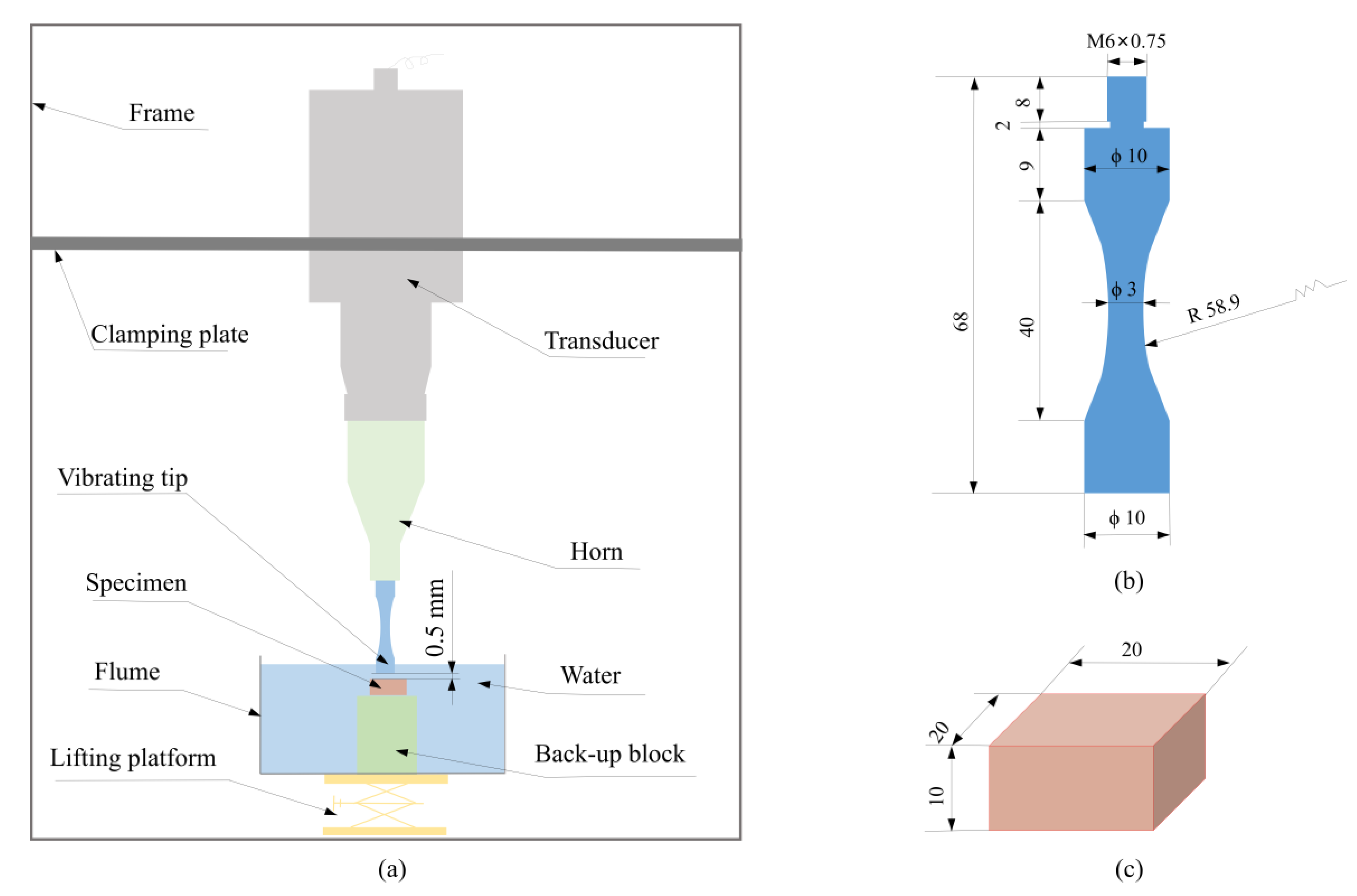
2.1. Experimental Program

The cavitation erosion test was conducted by using a modified ultrasonic fatigue apparatus according to ASTM G32-03 [31]. Cavitation bubbles were produced under a vibrating tip. The frequency of vibration was 20 ± 0.2 kHz. The peak-to-peak amplitude was 50 ± 0.6 μm. The vibrating tip was made of Ti-6Al-4V. The vibrating tip was immersed about 4 mm in tap water. The test was performed in running water with a stationary specimen method, as the stationary specimen method was convenient for characterizing eroded specimens. The standoff distance between specimen and tip was 0.5 mm. The specimen was placed under the vibrating tip. The vibrating tip introduced cavitation bubbles, the cavitation bubbles collapsed close to the specimens, and then specimens were eroded by the cavitation bubbles. The schematic image of the machine is shown in Figure 1. The temperature around the stationary specimen was kept at 25 ± 3 °C. As-received 420 and 316L were chosen as tested materials, their chemical compositions and mechanical properties are listed in Table 1 and Table 2, respectively. Specimens (20 mm × 20 mm × 10 mm) were made using wire electrical discharge machining. Specimens were ground and polished before they were taken to the cavitation erosion test. After the test, specimens were cleaned and dried by hot air, then the mass loss of the materials was weighed by an electronic balance with an accuracy of 0.1 mg. The eroded surfaces of specimens after different cavitation times are shown in Figure 2. For characterization, residual stress measurements were conducted on the eroded surface via X-ray diffraction. Three points were tested at different distances from the erosion center (0, 2, and 4 mm), then the average values and errors were calculated. Roughness was measured by a roughness measuring instrument. The microhardness test was carried out on a cross-section of the eroded specimen using a Vickers microhardness tester under loads of 100 gf and 200 gf for 316L and 420, respectively, with a dwell time of 15 s. The tested points were about 100 μm from the eroded surface.
In order to quantitatively study the relationship between cavitation damage and the parameters of cavitation time, roughness, residual stress, and microhardness, the mean depth of erosion (MDE) was used to describe cavitation damage, and it was calculated by using the following equation:
MDE = 1000 Δ m ρ A ,
where Δm is the mass loss (mg), ρ is the density of the materials (mg/mm3), and A is the area of eroded surface (mm2).

2.2. Significant Parameters of Cavitation Damage

The relationship between cavitation damage (mean depth of erosion) and cavitation time for 316L and 420 is presented in Figure 3a. In general, the cavitation damage of 316L and 420 increased with cavitation time. The cavitation damage evolution of 316L was similar to that of 420. The relationship between cavitation damage and average roughness of the eroded surface of 316L and 420 is presented in Figure 3b. Roughness increased with cavitation time because cavitation damage became increasingly serious; this was also found locally in other cavitation erosion processes [32,33,34,35]. On the whole, cavitation damage was proportional to roughness. The evolution rate of cavitation damage of 420 with roughness was faster than that of 316L. The relationship between cavitation damage and hardness of 316L and 420 is shown in Figure 3c. Because of the non-monotonic relationship between hardness and cavitation damage, especially for 316L, cavitation damage was not directly connected to hardness. The relationship between cavitation damage and residual stress is displayed in Figure 3d. It can be found that the residual stress of 316L was lower than that of 420 during CE. Meanwhile, cavitation damage of 316L and 420 increased overall with residual stress.

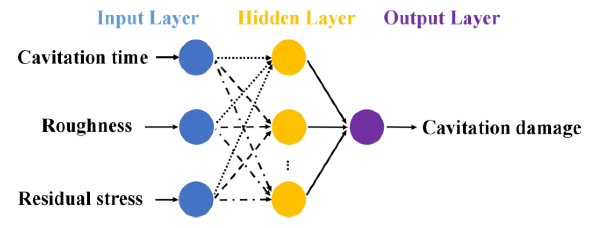
3. Artificial Neural Network (ANN) Approach

3.1. Back-Propagation Neural Network

ANN is an algorithmic, mathematical model for distributed, parallel information processing. It adjusts connections between a large number of internal nodes, according to the complexity of the system, to achieve the purpose of processing information. ANN has the ability of self-learning and self-adaptation. Back-propagation (BP) neural network is a kind of supervised feed-forward neural network. The processing units in the BP neural network include input layer, output layer, and several hidden layers. Units in the hidden layer are used to compute the weights between pattern, the error between generated output, and the targeted output is fed backward to modify its weight [24]. BP is widely applied because it is able to deal with complex, nonlinear mapping. It is particularly suitable for solving complex problems with internal mechanisms. Therefore, BP was adopted in this paper.
BP requires that the activation function used by the artificial nodes be differentiable, thus, logsig and tansig were utilized as the activation functions in the hidden layer. The activation function of purelin was used by default in the output layer. Although the result of the Levenberg-Marquardt training approach may be trapped in the local optima [23], needing larger storage space than other training algorithms, application of the Levenberg-Marquardt training approach in BP usually gets better results than other training algorithms, and its convergence rate is fast; thus, it is often applied.

3.2. Damage Prediction Using ANN

Parameters that influenced cavitation damage were used as the network input nodes, and the mean depth of erosion was used as the output. Besides the input and output layers, the hidden layer was included in BP. Generally, one or more layers could be utilized as hidden layers in the BP neural network. As there were not many input and output nodes, and one hidden layer was used in many applications with a desired accuracy [36], one hidden layer was adopted in this work. The number of hidden nodes could be estimated by Kolmogorov’s theorem [37],
N h = 2 N i + 1 ,
where Ni is the number of input nodes, and Nh is the number of hidden nodes. Then, the number of layers and the number of the nodes of each layer were confirmed.
As surface roughness and residual stress were related to cavitation damage, cavitation time affected the damage as well. Therefore, cavitation time, roughness, and residual stress could be used as input nodes, namely, the largest of the number of input nodes Ni could be set as 3, and Nh could be set as 7 according to the Equation (2). The mean depth of erosion represented the output node, namely, there was one output in the network, as is shown in Figure 4. The linear interpolation method was used to obtain enough instances from the tested data. There were 48 sets of data for inputs and outputs. Among those data, 42 groups of instances were selected randomly to model the network, 26 (about 60%) instances were used for training, 8 (about 20%) for validation, and the other 8 for testing the network. Besides, the remaining six instances were used to test the network model. The ANN architecture of three input nodes is shown in Figure 4.
Initial data of the connection weight coefficients of the layers were given by random numbers. Training was terminated when the average squared error between the network output and the target output was less than 0.00001. The maximum number of epochs was set as 500, and the learning rate was set as 0.05. The algorithm was written in MATLAB. The Neural Network toolbox was utilized to define, train, and simulate the network model. The built network model was repeated 50 times to check prediction accuracy and capability. To determine the performance of the network model, three different criteria were used: the relative absolute mean error (RAME), the root mean square error (RMSE), and the coefficient of determination (R2) [29,38]. The equations of these criteria are as follows:
RAME = 1 n i = 1 n | y p i y i y p i | ,
RMSE = i = 1 n ( y p i y i ) 2 n ,
R 2 = ( n i = 1 n y i y p i i = 1 n y i i = 1 n y p i n i = 1 n y i 2 ( i = 1 n y i ) 2 n i = 1 n y p i 2 ( i = 1 n y p i ) 2 ) 2 ,
where ypi is the predicted value, yi is the target value, and n is the number of instances. As the mean depth of erosion in the initial stage was zero, thus, the predicted value was used as the denominator of RAME.

4. Results and Discussion

As is shown in Figure 3, cavitation time and roughness were proportional to cavitation damage. Cavitation damage could be expressed by the mean depth of erosion according to Equation (1), as residual stress was considered an important factor for cavitation erosion behavior, and it had the tendency to increase with the cavitation damage; therefore, cavitation time, roughness, and residual stress were used as input nodes for cavitation damage prediction using ANN. To evaluate and improve the prediction accuracy of the ANN model, the effect of the number and type of input nodes, the number of nodes in the hidden layer, and different activation functions on prediction were analyzed. RAME, RMSE, and R2 were considered the evaluation criteria.

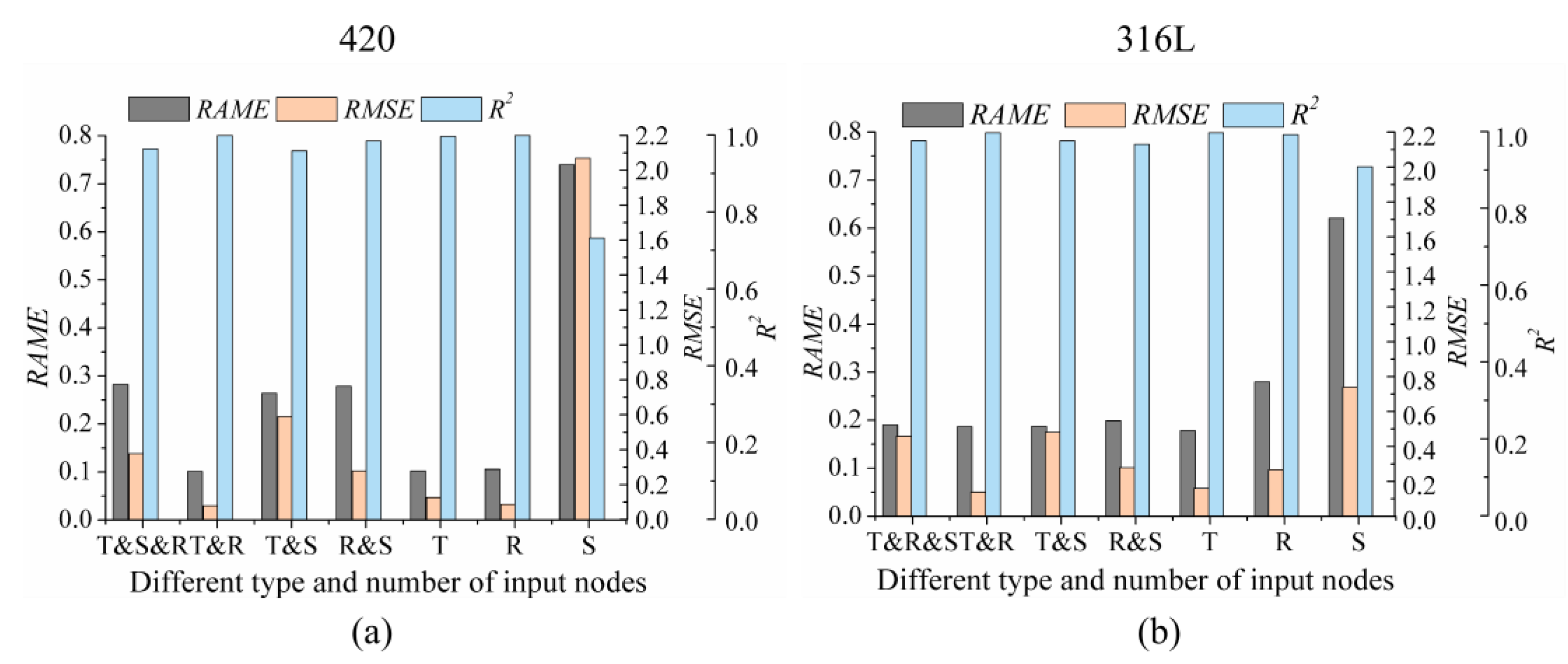
4.1. The Effects of Type and Number of Input Nodes on Prediction

Figure 5 presents the effect of type and the number of input nodes on cavitation damage prediction for 420 and 316L. The number of nodes in the hidden layer of all models was seven in Figure 5. It seemed that the number of input nodes did not affect prediction results. But for the type of input nodes, it was apparent that the worst performance was in the model with the residual stress input node. This was probably because the value of residual stress was not accurate, as the measurement of residual stress was affected by the roughness of the eroded surface. Relatively good performances were achieved by the model with cavitation time and roughness (T&R) input nodes and the model with the input node of cavitation time (T). To analyze the best performance of models with different input nodes, RAME, RMSE, and R2 values for models with T&R and T are shown in Table 3. Regardless of the similar criteria results, RAME, R2 of the model with 420, and R2 of the model with 316L showed that the best performance was achieved by the model with the input nodes of cavitation time and roughness (T&R), as the prediction model using the input nodes of T&R had smaller RMSE values.

4.2. The Effects of the Number of Nodes in the Hidden Layers on Prediction

It has been suggested that the number of nodes in the hidden layer influences the results of the ANN model, and that usually the more nodes there are in the hidden layer the better the ANN performance [39]. RAME, RMSE, and R2 for different numbers of nodes in the hidden layer and different numbers and types of input nodes are presented in Figure 6. For one input node, the input node of residual stress (S) was not analyzed for its worst performance, shown in Figure 5. In Figure 6a,b it was interesting to find that on the whole, for models with input node, cavitation time (T), and roughness (R), the performances of these two models became increasingly worse with the increase of node number in the hidden layer. The best performance was achieved by the model with the input node of cavitation time (T) and seven nodes in the hidden layer, as shown in Figure 6a,b. For models with three and two input nodes, results of their criteria were irregular, as displayed in Figure 6c,d. But it could be seen that the best performance was achieved by the model with the input nodes of cavitation time and roughness (T&R) and eleven nodes in the hidden layer, and that the best performance of models with three input nodes (cavitation time, roughness, and residual stress (T&R&S)) was in the model with three nodes in the hidden layer, as shown in Figure 6e,f.

4.3. The Effects of Activation Functions on Prediction

From the above analysis it was seen that for the models with three input nodes (cavitation time, roughness, and residual stress (T&R&S)), the best performance was in the model with three nodes in the hidden layer (T&R&S-3); for the models with two input nodes, the best performance was achieved in the model with the input nodes of cavitation time and roughness and eleven nodes in the hidden layer (T&R-11); and for the models with one input node, the best performance was obtained by the model with the input node of cavitation time and seven nodes in the hidden layer (T-7). To further improve the accuracy of prediction, the effect of different activation functions on the prediction is shown in Figure 7. It was drawn that the activation function of logsig could slightly improve the accuracy of prediction. The best performance was in the model with the input nodes of cavitation time and roughness, eleven nodes in the hidden layer, and the activation function of logsig (T&R-11-logsig)—the criteria results of this model, RAME, RMSE, and R2 were about 0.17, 0.13, and 0.999, respectively.

5. Conclusions

In this paper, it can be found that there are relationships between cavitation damage and the parameters including cavitation time, roughness, and residual stress. ANN modeling of cavitation damage of 420 and 316L is investigated based on this relationship, and the following conclusions can be drawn:
(1)
A prediction approach using the artificial neural network for the cavitation damage is proposed.
(2)
From the analysis of the relationship between cavitation damage and microhardness, microhardness seems not to be related to cavitation damage.
(3)
From analysis of the relationship between cavitation damage, residual stress, and the ANN model, residual stress seems not to be related to cavitation damage.
(4)
Cavitation damage is affected by cavitation time and roughness. The increase of cavitation time or the increase of roughness during the cavitation erosion process increases cavitation damage.
(5)
The model using BP method with input nodes of cavitation time and roughness, eleven nodes in the hidden layer, and the activation function of logsig has a good performance of forecasting cavitation damage.

Author Contributions

G.G. wrote this paper, Z.Z., C.C., J.Z. and B.N. reviewed this paper.

Funding

This work is funded by the National Key Research and Development Program of China, grant number: 2016YFF0203301.

Acknowledgments

The authors would like to thank Luowei Cao from China Special Equipment Inspection and Research Institute, for his offering the material and testing the chemical composition and mechanical properties of 316L and 420.

Conflicts of Interest

The authors declare no conflict of interest.

References

  1. Brennen, C.E. Hydrodynamics of Pumps; Jiangsu University Press: Zhenjiang, China, 2012; pp. 1–52. [Google Scholar]
  2. Naudé, C.F.; Ellis, A.T. On the mechanism of cavitation damage by non-hemispherical cavities collapsing in contact with a solid boundary. J. Basic Eng. 1960, 83, 648–656. [Google Scholar] [CrossRef]
  3. Dojcinovic, M.; Eric, O.; Rajnovic, D.; Sidjanin, L.; Balos, S. Effect of austempering temperature on cavitation behaviour of unalloyed ADI material. Mater. Charact. 2013, 82, 66–72. [Google Scholar] [CrossRef]
  4. Zhen, L.; Han, J.; Lu, J.; Chen, J. Cavitation erosion behavior of Hastelloy C-276 nickel-based alloy. J. Alloy. Compd. 2015, 619, 754–759. [Google Scholar]
  5. Kim, K.H.; Chahine, G.; Franc, J.P.; Karimi, A. Advanced Experimental and Numerical Techniques for Cavitation Erosion Prediction; Springer: New York, NY, USA, 2014. [Google Scholar]
  6. Hattori, S.; Hirose, T.; Sugiyama, K. Prediction method for cavitation erosion based on measurement of bubble collapse impact loads. Wear 2009, 269, 507–514. [Google Scholar] [CrossRef]
  7. Szkodo, M. Mathematical description and evaluation of cavitation erosion resistance of materials. J. Mater. Process. Tech. 2005, 164, 1631–1636. [Google Scholar] [CrossRef]
  8. Hattori, S.; Maeda, K.; Zhang, Q. Formulation of cavitation erosion behavior based on logistic analysis. Wear 2004, 257, 1064–1070. [Google Scholar] [CrossRef]
  9. Shuji, H.; Kohei, M. Logistic curve model of cavitation erosion progress in metallic materials. Wear 2010, 268, 855–862. [Google Scholar]
  10. Wang, Y.; Stella, J.; Darut, G.; Poirier, T.; Liao, H.L.; Planche, M.P. APS prepared NiCrBSi-YSZ composite coatings for protection against cavitation erosion. J. Alloys Compd. 2017, 699, 1095–1103. [Google Scholar] [CrossRef]
  11. Emelyanenko, A.M.; Shagieva, F.M.; Domantovsky, A.G.; Boinovich, L.B. Nanosecond laser micro- and nanotexturing for the design of a superhydrophobic coating robust against long-term contact with water, cavitation, and abrasion. Appl. Surf. Sci. 2015, 332, 513–517. [Google Scholar] [CrossRef]
  12. Wang, Y.; Liu, J.W.; Kang, N.; Darut, G.; Poirier, T.; Stella, J.; Liao, H.L.; Planche, M.P. Cavitation erosion of plasma-sprayed CoMoCrSi coatings. Tribol. Int. 2016, 102, 429–435. [Google Scholar] [CrossRef]
  13. Lin, J.R.; Wang, Z.H.; Lin, P.H.; Cheng, J.B.; Zhang, X.; Hong, S. Effects of post annealing on the microstructure, mechanical properties and cavitation erosion behavior of arc-sprayed FeNiCrBSiNbW coatings. Mater. Des. 2015, 65, 1035–1040. [Google Scholar] [CrossRef]
  14. Kumar, A.; Sharma, A.; Goel, S.K. Effect of heat treatment on microstructure, mechanical properties and erosion resistance of cast 23-8-N nitronic steel. Mater. Sci. Eng. 2015, 637, 56–62. [Google Scholar] [CrossRef]
  15. Wang, Z.; Zhu, J. Correlation of martensitic transformation and surface mechanical behavior with cavitation erosion resistance for some iron-based alloys. Wear 2004, 256, 1208–1213. [Google Scholar] [CrossRef]
  16. Thiruvengadam, A.; Waring, S. Mechanical Properties of Metals and Their Cavitation Damage Resistance; Technical Report 233-5; Hydronautics Inc.: Laurel, MD, USA, 1 June 1964; p. 47. [Google Scholar]
  17. Duraiselvam, M.; Galun, R.; Wesling, V.; Mordike, B.L.; Reiter, R.; Oligmüller, J. Cavitation erosion resistance of AISI 420 martensitic stainless steel laser-clad with nickel aluminide intermetallic composites and matrix composites with TiC reinforcement. Surf. Coat. Technol. 2006, 201, 1289–1295. [Google Scholar] [CrossRef]
  18. Mottyll, S.; Skoda, R. Numerical 3D flow simulation of ultrasonic horns with attached cavitation structures and assessment of flow aggressiveness and cavitation erosion sensitive wall zones. Ultrason. Sonochem. 2016, 31, 570–589. [Google Scholar] [CrossRef]
  19. Brennen, C.E. Cavitation and Bubble Dynamics; Oxford University Press: New York, NY, USA, 1995; pp. 71–85. [Google Scholar]
  20. Schijve, J. Fatigue of Structures and Materials, 2nd ed.; Aviation Industry Press: Beijing, China, 2004; pp. 11–363. [Google Scholar]
  21. Pędzich, Z.; Jasionowski, R.; Ziąbka, M. Cavitation wear of structural oxide ceramics and selected composite materials. J. Eur. Ceram. Soc. 2014, 34, 3351–3356. [Google Scholar] [CrossRef]
  22. Choi, J.K.; Chahine, G.L. Relationship between material pitting and cavitation field impulsive pressures. Wear 2016, 352–353, 42–53. [Google Scholar] [CrossRef]
  23. Hsu, K.L.; Gupta, H.V.; Sorooshian, S. Artificial neural network modeling of the rainfall-runoff process. Water Resour. Res. 1995, 31, 2517–2530. [Google Scholar] [CrossRef]
  24. Jeyasehar, C.A.; Sumangala, K. Damage assessment of prestressed concrete beams using artificial neural network (ANN) approach. Comput. Struct. 2006, 84, 1709–1718. [Google Scholar] [CrossRef]
  25. Ye, L.; Su, Z.; Yang, C.; He, Z.; Wang, X. Hierarchical development of training database for artificial neural network-based damage identification. Compos. Struct. 2006, 76, 224–233. [Google Scholar] [CrossRef]
  26. Zang, C.; Imregun, M. Structural damage detection using artificial neural networks and measured FRF data reduced via principal component projection. J. Sound Vib. 2001, 242, 813–827. [Google Scholar] [CrossRef]
  27. Strdczkiewicz, M.; Barszcz, T. Application of artificial neural network for damage detection in planetary gearbox of wind turbine. Shock Vib. 2015, 2016, 1–12. [Google Scholar]
  28. Xu, H.; Humar, J.M. Damage detection in a girder bridge by artificial neural network technique. Comput. Civ. Infrastruct. Eng. 2010, 21, 450–464. [Google Scholar] [CrossRef]
  29. Altarazi, S.; Ammouri, M.; Hijazi, A. Artificial neural network modeling to evaluate polyvinylchloride composites’ properties. Comput. Mater. Sci. 2018, 153, 1–9. [Google Scholar] [CrossRef]
  30. Adoption, P.N. Centrifugal Pumps for Petroleum, Petrochemical and Natural Gas Industries; API Publishing Services: Washington, DC, USA, 2003. [Google Scholar]
  31. Astm, N.G. Standard Test Method for Cavitation Erosion Using Vibratory Apparatus; ASTM: West Conshohocken, PA, USA, 2003. [Google Scholar]
  32. Karimi, A.; Martin, J.L. Cavitation erosion of materials. Metall. Rev. 2013, 31, 1–26. [Google Scholar] [CrossRef]
  33. Santa, J.F.; Blanco, J.A.; Giraldo, J.E. Cavitation erosion of martensitic and austenitic stainless steel welded coatings. Wear 2011, 271, 1445–1453. [Google Scholar] [CrossRef]
  34. Xiaojun, Z.; Procopiak, L.A.J.; Souza, N.C.; D’Oliveira, A.S.C.M. Phase transformation during cavitation erosion of a Co stainless steel. Mater. Sci. Eng. A 2003, 358, 199–204. [Google Scholar] [CrossRef]
  35. Li, D.G.; Wang, J.D.; Chen, D.R.; Liang, P. Ultrasonic cavitation erosion of Ti in 0.35% NaCl solution with bubbling oxygen and nitrogen. Ultrason. Sonochem. 2015, 26, 99–110. [Google Scholar] [CrossRef]
  36. Hugo, V.; De Albuquerque, C.; Tavares, M.R.S.; Durão, L.M.P.; João, P. Evaluation of Delamination Damage on Composite Plates using an Artificial Neural Network for the Radiographic Image Analysis. J. Compos. Mater. 2010, 44, 548–553. [Google Scholar]
  37. Kůrková, V. Kolmogorov’s theorem and multilayer neural networks. Neural Networks 1992, 5, 501–506. [Google Scholar] [CrossRef]
  38. Singh, K.P.; Basant, A.; Malik, A.; Jain, G. Artificial neural network modeling of the river water quality—A case study. Ecol. Modell. 2009, 220, 888–895. [Google Scholar] [CrossRef]
  39. Chen, M. Neural Network Principle and Example Elaboration of MATLAB; Tsinghua University Press: Beijing, China, 2003; pp. 21–157. [Google Scholar]
Figure 1. (a) Schematic image of the machine, (b) shape and size of the vibrating tip, and (c) shape and size of the specimen. (Unit: mm).
Metals 09 00506 g001
Figure 2. Eroded surfaces of specimens of 420 after different cavitation times: (a) 10 min, (b) 30 min, (c) 60 min, (d) 120 min, (e) 180 min, and (f) 240 min.
Metals 09 00506 g002
Figure 3. (a) Cavitation time, (b) roughness, (c) microhardness, and (d) residual stress as a function of the mean depth of erosion of 420 and 316L.
Metals 09 00506 g003
Figure 4. Structure for models with the input nodes of cavitation time, roughness, and residual stress (T&R&S).
Metals 09 00506 g004
Figure 5. Relative absolute mean error (RAME), root mean square error (RMSE), and R2 for models with different numbers and types of input nodes and different stainless steels (a) 420 and (b) 316L.
Metals 09 00506 g005
Figure 6. RAME, RMSE, and R2 for models with different numbers of nodes in the hidden layer: (a,b) one input node, (c,d) two input nodes, and (e,f) three input nodes.
Metals 09 00506 g006
Figure 7. Criteria for models with different activation functions: (a) RAME and RMSE and (b) R2.
Metals 09 00506 g007
Table 1. Chemical compositions of 420 and 316L.
MaterialChemical Composition
CCrNiMnSiMoPSNFe
4200.2012.100.280.340.29-0.0260.015-Bal.
316L0.01916.9610.520.950.372.140.0450.00270.036Bal.
Table 2. Mechanical properties of 420 and 316L.
MaterialYield Strength σ0.2 (MPa)Tensile Strength (MPa)Vickers Microhardness (HV)Density (g/cm3)
4205367051857.85
316L4016511527.98
Table 3. RAME, RMSE, and R2 for the models with input nodes of T&R and the models with input node of T in Figure 3.
Stainless Steels420316L
Input NodesCriteria
RAMERMSER2RAMERMSER2
T&R0.10150.07970.99900.18680.13850.9968
T0.10200.08660.99930.17850.16160.9971

