Abstract
The mechanical performances and microstructure of Ti–6Al–4V built by selective laser melting were evaluated by optical microscopy, transmission electron microscopy, and room temperature tensile testing, and compared with the wrought and as-cast material. The flow behavior of the as-produced Ti–6Al–4V at temperatures varying from 700–900 °C at an interval of 50 °C and strain rates ranging from 10−2–101 s−1 was experimentally acquired. According to the experimental measurement, the Johnson–Cook, modified Arrhenius model, and artificial neural network were constructed. A comparative investigation on the predictability of established models was performed. The as-produced microstructure is made up of non-equilibrium martensite and columnar grains, leading to higher strength and lower ductility with respect to the conventional material. In room temperature tensile tests, the SLMed Ti–6Al–4V shows the characteristics of continuous yielding and unobvious work-hardening. The flow stress rapidly reaches the peak, and the softening rate depends on the strain rates and deformed temperatures in hot compression. The Johnson–Cook model could well predict the flow stress during quasi-static tensile deformation, but the model constants might vary with the process conditions. For dynamic compression, the artificial neural network exhibits higher accuracy to fit the flow stress of SLMed Ti–6Al–4V, and higher error to predict the conditions out of the model data, compared to the modified Arrhenius model involving the compensation of strain rate and strain.
1. Introduction
Ti–6Al–4V alloy is one of the commonly used titanium alloys, which has been extensively applied in military, biomedical, energy, automotive, and chemical industries [1]. This is mainly attributed to its high specific strength, outstanding biocompatibility, excellent corrosion resistance, and high-temperature mechanical properties. However, the high cost from metallurgical extraction and fabrication by traditional processing techniques seriously restricts its broader employment in various industries [2]. In recent years, the emerging selective laser melting process could rapidly form free-shaped Ti–6Al–4V alloy components with high material utilization, which offers individuals alternative economic and efficient approaches to fabricate metal products on demand [3].
In the SLM process, a high energy laser beam travels in the powder bed along the pre-set scanning path, and fine powder particles are melted into almost completely dense parts. Due to its layer-wise deposition, the SLM process could fabricate complex geometry components with which traditional processing technologies could not compete. It is the obvious advantages mentioned above that attract more and more attention from academia and industry. Currently, the SLM process has been successfully employed in fabricating various customized implants [4], lightweight structures [5], and other complicated end-usable metal parts such as fuel nozzles with improved performance [6].
In the past few decades, great efforts have been devoted to investigating the relationship between the processing parameters, microstructure, and mechanical properties of Ti–6Al–4V produced by SLM. Sun et al. [7] optimized the process parameters to maximize the densification of SLM-deposited Ti–6Al–4V using the statistical analysis method and obtained fully densified Ti–6Al–4V under optimal process parameters. Yang et al. [8] characterized the microstructure of SLM-fabricated Ti–6Al–4V in detail and explored the formation of an α’martensite. Owing to the brittle and anisotropic microstructure, the as-built Ti–6Al–4V alloy has a higher tensile strength compared to the hot-worked material, but a lower ductility dependent on the building orientation [9,10]. For load-bearing structural parts, the dynamic mechanical properties such as fatigue resistance are still one of the major concerns of mechanical engineers. The as-printed Ti–6Al–4V has considerably lower fatigue life with respect to the wrought material, which should be attributed to the residual stress, internal porosity, low surface quality, and microstructure [11]. To enhance the mechanical performance, various heat treatments [12,13] have been attempted to eliminate the residual stress and regulate the microstructure, hot isostatic pressing (HIP) [14] was applied to close the internal defects, and surface post-treatment [15] including shot peening, electro-polishing, sandblasting, and machining was adopted to decrease the surface roughness. After surface finishing and heat post-treatments such as HIP, the fatigue performance of SLM-deposited Ti–Al–4V could be equivalent to that of the wrought material. In addition to steel, this alloy is currently the most investigated SLM-fabricated metallic material.
However, by reviewing the work of predecessors, it could be found that limited investigations [16,17] were carried out to understand the dynamic stress-strain behavior of SLMed Ti–6Al–4V, especially at elevated temperatures and strain rates with a wide range. Secondly, the microstructure of SLMed Ti–6Al–4V is quite distinctive from that of the material obtained by conventional ways, which derives from the rapid solidification process and complex thermal cycling history. The resulting mechanical features of SLMed Ti–6Al–4V should be distinct. Furthermore, there are only a few comparatively systematic research studies on constitutive modeling of SLMed metals and alloys, such as Ti–6Al–4V [18,19]. Lu et al. [20] established a three-dimensional (3D) thermomechanical coupled finite element model for laser additive manufacturing (LAM) of Ti–6Al–4V, discussed the sensitivity of the mechanical parameters published in the literature, and pointed out that the material data of Ti–6Al–4V from traditional processes were not suitable for the simulation of LAM. In order to predict the residual stress and deformation behavior accurately during the SLM of Ti–6Al–4V, it is necessary to establish the related mathematical models of SLMed Ti–6Al–4V. Hence, the main purpose of the current work is to understand the dynamic thermomechanical response of SLM-manufactured Ti–6Al–4V and develop the corresponding constitutive equations to depict the alloy’s mechanical behavior. In this paper, the comparison of microstructure and room temperature mechanical properties between SLMed, as-cast, and forged Ti–6Al–4V alloy was conducted. Next, the thermal compression at constant strain rates from 10−2–101 s−1 was performed at the temperatures from 700–900 °C. The flow stress of the SLMed Ti–6Al–4V alloy was predicted by the phenomenological and intelligent models. The constitutive models could be available to modelers to conduct a relatively accurate finite element analysis of SLM-built Ti–6Al–4V alloy components.
2. Materials and Methods
Dozens of cylindrical bars (height: 80 mm, diameter: 12 mm) with horizontal and vertical orientations were fabricated in an EOS 280 SLM equipment (EOS, Maisach, Germany). The spherical powder of the pre-alloyed Ti–6Al–4V ranging from 23–56 µm in size was employed as shown in Figure 1. The oxygen content in the building chamber was controlled to be lower than 0.1%. The baseplate temperature was about 35 °C. The laser power was 280 W. The powder layer thickness was 30 μm. The hatch spacing was 140 μm. The laser scan speed was 1200 mm/s. The zigzag scanning pattern was employed, and the laser scan direction in the newly-deposited layer was rotated by 67° with respect to the scan direction of the previous layer. The fully densified parts were achieved using the above-mentioned parameters. Metallographic samples were obtained by conventional mechanical methods and etched with Kroll reagent. The macrostructure of the as-built material was observed using a Zeiss optical microscope (OM) (Zeiss, Haydenheim, Germany). For a detailed analysis of the microstructural features, a transmission electron microscope (TEM) (FEI, Hillsboro, OR, USA) was adopted.
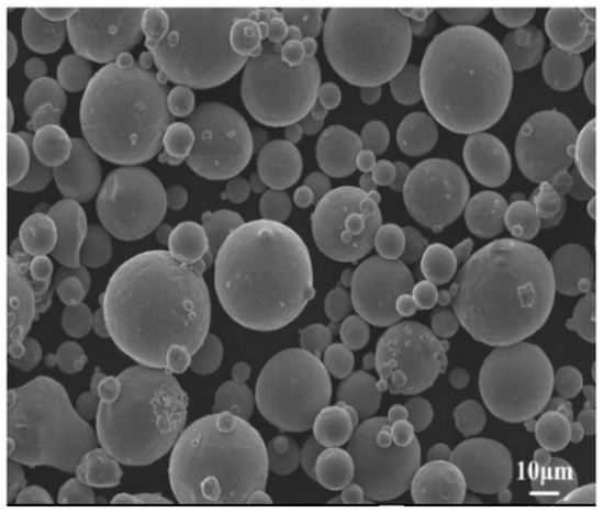
Figure 1.
Surface morphology of the Ti–6Al–4V alloy spherical powder particles.
Unidirectional tensile tests at room temperature were carried out on an electronic universal material testing machine (Instron, Boston, MA, USA) equipped with a tensile extensometer under a strain rate of 10−3 s−1. Prior to the compression, small cylinders shown in Figure 2b (height: 12 mm, diameter: 8 mm) were obtained by machining. Hot compression using vertically-oriented samples was implemented on a thermal-mechanics simulator Gleeble-1500 (DSI, New York, NY, USA) as displayed in Figure 2a. The compression strain rates were 10−2 s−1, 10−1 s−1, 100 s−1, and 101 s−1. The compression temperature was in the range of 700–900 °C at 50 °C intervals. The thermocouple wires were welded to the center of the cylinders by energy storage welding to measure the temperature of specimens during deformation. A thin graphite sheet was placed between the specimen and the indenter to lubricate and prevent the cylinder from bonding to the indenter at high temperatures. The small cylinders were rapidly heated to the predetermined temperatures at a heating rate of 10 °C/s and then kept for about half a minute. The total height reduction was about 60% at the end of deformation.
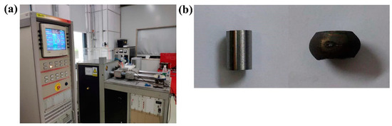
Figure 2.
(a) Images of the thermal simulator Gleeble-1500 and (b) a small cylinder before and after compression.
3. Results and Discussion
3.1. Microstructure and Properties of SLMed Ti–6Al–4V Alloy
Figure 3 shows the microstructure of SLM-printed Ti–6Al–4V. The 3D macrostructure is composed of prior columnar β grains with an average width 139.7 ± 11.2 μm as shown in Figure 3a, which grow through several deposited layers and are nearly parallel to the deposition orientation. Columnar crystals are originated from the epitaxial growth of the β grains in the deposited layers that have already been solidified. For a high cooling rate up to 1 × 10⁶ °C/s during the deposition [21], the newly-formed β phases after solidification are almost completely transformed to needlelike α′ martensite by shear transformation. The columnar β grains are covered with large numbers of intercross-aligned martensitic laths as shown in Figure 3b. In addition, large amounts of crystal defects such as twins and dislocations are also observed. It is well-known that large internal stress frequently arises in SLM-fabricated components due to the steep temperature gradient and the high cooling rate. Due to fewer slip systems in the Ti–6Al–4V alloy with close-packed hexagonal structures, the deformation of SLMed parts is usually accompanied with a dislocation slip and twinning deformation [22]. If the accumulated stress in the matrix is beyond the critical shear stress at which twinning occurs, twinning deformation begins, and twins emerge. Consequently, the as-fabricated Ti–6Al–4V alloy possesses high strength and low ductility. As shown in Table 1, the yield stress of as-printed Ti–6Al–4V is 1036–1187 MPa and the ultimate strength is about 1300 MPa on average, while the average elongation to failure is 6.8–8.7% and the average reduction of the area is 21.3–28.6%.
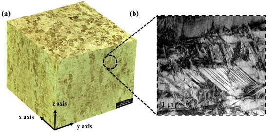
Figure 3.
The microstructure of the as-built Ti–6Al–4V alloy: (a) 3D optical microscope (OM) microstructure, (b) transmission electron microscope (TEM) microstructure. The z-axis direction is the building direction.

Table 1.
The mechanical properties at room temperature of the Ti–6Al–4V alloy produced by SLM and traditional processes.
Compared with the as-built, the as-cast material as shown in Figure 4a consists of coarse equiaxed prior β grains and straight (α + β) lamellas, resulting from the slow cooling rate during the investment casting. The cooling rate of investment casting of the Ti–6Al–4V alloy is generally around 1 °C/s. The average size of the coarse prior β grains measured by the linear intercept method is about 1.07 ± 0.24 mm. According to the well-known Hall–Petch relationship, the strength of the metals and alloys is in inverse proportion to the effective grain size. As expected, the strength of the Ti–6Al–4V alloy by casting is significantly lower than as-printed counterparts as displayed in Table 1. The yield and tensile strength of the as-cast material are only about 776 MPa and 881 MPa, respectively. For the wrought Ti–6Al–4V, some segments of the original β grain boundaries could be distinguished by the bright white grain boundary α phases as shown in Figure 4b. The thin grain boundary α phases formed in the slow cooling process after forging are considered to be harmful to mechanical performances [23]. The distorted (α + β) clusters are distributed in the prior β grains due to intense plastic deformation.
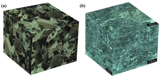
Figure 4.
The (a) as-cast and (b) as-forged microstructure of the Ti–6Al–4V alloy.
For a brief description, SLM-V/H means that the samples were built with vertical/horizontal orientation during SLM. The mechanical properties include the modulus of elasticity (E), elongation to failure (EL), yield stress (σ0.2), ultimate tensile stress (σu), and reduction of area (R/A).
3.2. Flow Behavior
Figure 5 illustrates the quasi-static flow stress-strain curves of Ti–6Al–4V produced by SLM, 3D laser deposition, and conventional process technologies [24]. All the curves have similar elastic modulus and exhibit continuous yield behavior without obvious work-hardening. The SLMed Ti–6Al–4V alloys have higher yield strength than the same material obtained from other process routes. It could also be seen that the measured SLMed curves in this study are different from the SLMed curves in reference [17]. The deviation could have resulted from the difference in used powders, process parameters, and printing machines. At present, building consistency and performance stability are still one of the challenges in the process of large-scale industrial applications of SLMed products. In the measured SLMed curves, the anisotropy between horizontally and vertically-oriented samples is observed, which relies on the orientation relationship between the loading direction and the long axis of the columnar grains and defects.
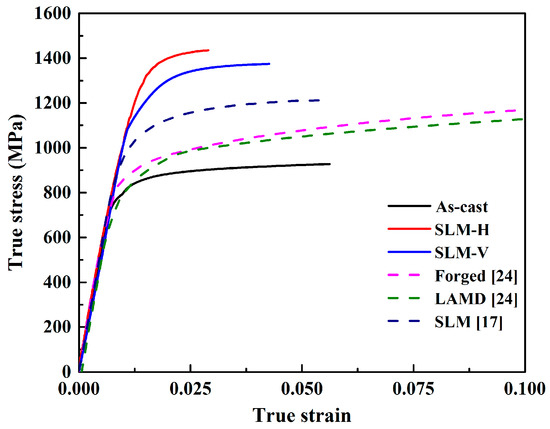
Figure 5.
The quasi-static stress-strain curves comparison among the SLMed, the 3D laser deposited, and the conventional Ti–6Al–4V alloy.
Figure 6 demonstrates the measured true stress-strain curves. The flow stress under all process conditions rapidly peaks at a relatively small strain and then is followed by extensive flow softening. Matsumoto et al. [25] investigated the microstructural conversion mechanism of the Ti–6Al–4V alloy with the martensite microstructure at a compression temperature of 700 °C and a strain rate of 10 s−1, and pointed out that the rapid stress softening after peak stress was attributed to the formation of sub-grains in the martensite laths or at the interfaces of martensite laths and the high-speed fragmentation of grains during deformation. They also found that the softening rate was higher than that of the Ti–6Al–4V alloy with equilibrium (α + β) dual-phase microstructure because of large amounts of crystal defects such as dislocations, interfaces, and twins in the martensitic microstructure. These defects can provide nucleation sites for newly-formed grains. It could be seen in Figure 6 that the stress-strain curves after peak stresses at temperatures less than 800 °C are almost parallel, while the rate of stress softening decreases with the strain rate decrease at temperatures higher than 800 °C. It is well known that the decomposition of non-equilibrium α′ martensite is an atomic diffusion controlled process, which involves an incubation period before phase transition. Mur et al. [26] studied the transition kinetics of α′ to α + β and thought that the decomposition of α′ to α + β started when heated to temperatures above 400 °C, and was completed at 800 °C. Generally, the incubation period of diffusion transition is shortened as the transition temperature increases. Therefore, the deformed matrix could still be an α′ martensite at high strain rates even if the deformation temperature arrives at 800 °C because there is not enough time to decompose the α′ martensite into α + β phases before hot deformation. In contrast, the α′ martensite could be partially or completely converted into equilibrium (α + β) phases during the hot deformation at higher compression temperatures and lower strain rates, leading to relatively lower stress softening rates. Additionally, for the instability of the plastic flow [27], abnormal hardening is observed as indicated in the red rectangular dashed box in Figure 6c,d under the conditions of 800–850 °C and 1 s−1.
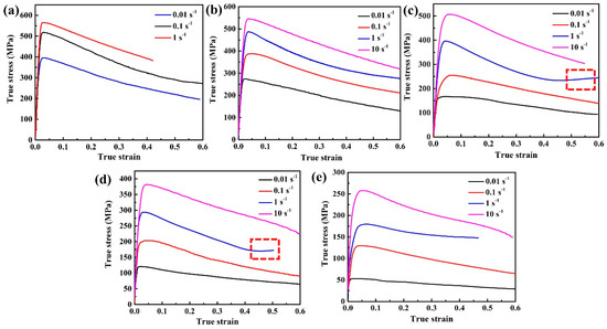
Figure 6.
Flow stress-strain curves of the SLMed Ti–6Al–4V alloy at different deformed temperatures higher than 700 °C: (a) 700 °C, (b) 750 °C, (c) 800 °C, (d) 850 °C, and (e) 900 °C.
3.3. Constitutive Modeling
To forecast the flow stress of metals accurately, individuals proposed various physical-based, phenomenological models and artificial neural networks (ANN) [28]. The Arrhenius model given by Sellars et al. [29] is usually used to depict the effects of strain rate and temperature on flow stress at high deformed temperatures. The Johnson–Cook (J–C) model could consider the effects of temperature, stain rate, and strain independently [30]. Therefore, in the following sections, the J–C model was utilized to predict the flow behavior at a strain rate of 10−3 s−1, and the dynamic hot compression process was predicted by the Arrhenius model. Furthermore, an ANN model was also developed for the dynamic compression process. Before mathematical modeling, the stress-strain data with abnormal hardening were discarded.
3.3.1. Quasi-Static Modeling
In the Johnson–Cook model, true stress could be described below:
where εp denotes the plastic strain, σ is the true stress (MPa), A0 is the yield strength (MPa) at the reference strain rate and temperature, B is the strain hardening coefficient, n0 represents the strain hardening exponent, m and C are the sensitivity coefficients of the temperature and strain rate, respectively, and ε* and T* represent the normalized strain rate and temperature as described below:
where Tm is the melting point of the alloy, and and Tr are the reference strain rate (s−1) and temperature (K), respectively. In this study, there is only one deformation temperature during the quasi-static process. Therefore, the J–C model could be simplified to the Equation (4).
The parameters B and n0 could be acquired by the intercept and slope of the curve vs. . The resulting model constants are listed in Table 2. The similar hardening exponentials of both models should be attributed to the same matrix microstructure.
Table 2.
The material constants in the J–C model for the SLMed Ti–6Al–4V alloy. Note that “SLM-R” represents the SLM curve of the reference.
The comparison between measurement and prediction is shown in Figure 7. The average absolute relative error (AARE) and correlation coefficient (R) are employed to verify the preciseness of the established models according to Equations (5) and (6):
where Ei represents the measured stress, Pi denotes the predicted value, and and are the average of the measurement and prediction, respectively. As shown in Table 3, the correlation coefficients are above 0.98, and the average absolute relative error is not higher than 2.5%, which implies excellent prediction ability of the established J–C model.
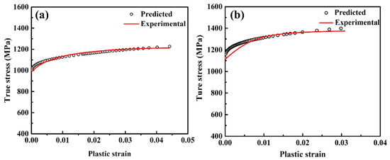
Figure 7.
Comparison between the predicted stresses by J–C model and experimental measurements: (a) SLM-R, (b) SLM-V.
Table 3.
The calculated values of ARRE and R for the J–C model.
3.3.2. Dynamic Modeling
- The Arrhenius Model
The detailed mathematical expressions of the Arrhenius model are given in Equations (7)–(10):
where , , , , , , and are material-related constants, , is the strain rate (s-1), is the universal gas constant (8.314 J/mol/K), is the absolute temperature (K), is the activation energy of deformation (J/mol), and represents the Zener–Hollomon parameter. Thus, the flow stress could be also represented as follows:
where the material constants could be determined by substituting Equation (7) into Equations (8)–(10) and taking the logarithm.
At a given temperature, the constants and were obtained by averaging the reciprocal of slopes of curves vs. and vs. according to Equations (12) and (13), respectively. The activation energy is the average of the slope of curves vs. and was determined by the intercepts of these curves for a given strain rate according to Equation (14). For accurate prediction, the strain compensation should be considered [31]. Subsequently, the related constants were computed in the strain range from 0.05–0.4 at the interval of 0.025 in the same manner. The relationship between the strain and material constants was fitted using a fifth-order polynomial according to Equation (15). The resulting fitted curves are shown in Figure 8. The fitted polynomial coefficients are listed in Table 4.
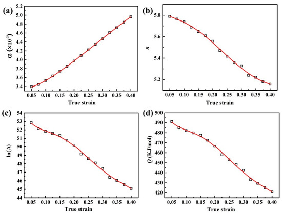
Figure 8.
The material constants that vary with the strain: (a) α, (b) n, (c) lnA, and (d) Q.
Table 4.
The resulting fitting coefficients of α, n, lnA, and Q of as-printed Ti–6Al–4V alloy.
After the material constants were determined, the flow stress could be predicted using Equations (7), (11), and (15). The predicted values by the Arrhenius model and experimental results are described in Figure 9. Despite a similar trend, large relative deviations still exist under certain processing conditions. Consequently, necessary improvements to the Arrhenius model are required.
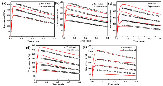
Figure 9.
Comparison between the predicted stresses by the Arrhenius model and the experimental ones: (a) 700 °C, (b) 750 °C, (c) 800 °C, (d) 850 °C, and (e) 900 °C.
From Figure 9, it could be found that the measured stress is lower than the predicted value when the strain rate is greater or equal to 1 s−1 and the deformed temperature is less than or equal to 750 °C. This overestimation could be attributed to the adiabatic heating during deformation. Large amounts of deformation heat would be generated during the rapid compression of the Ti–6Al–4V alloy, which cannot be dissipated in time because of its poor thermal conductivity, resulting in localized stress softening [32]. After trial and error, an adiabatic temperature rise of ΔT = 10 °C is added to the T in Z as displayed in Equation (16). Secondly, the underestimation is observed in Figure 9c,d for the strain rate greater than 10 s−1 and temperatures of 800–850 °C. The compensation of strain rate is considered by regulating the exponent of strain rate in Z as shown in Equation (17) according to that in Peng et al. [33]. While the temperature reaches 900 °C, the model could basically predict the change of flow stress except when the strain rate is 10−2 s−1 and 1 s−1. For the strain rate of 1 s−1, the deviation gradually increases with the strain if the true strain is greater than 0.2. It is difficult to directly determine the specific cause, or it may be from the test error. For the strain rate of 10−2 s−1, the measured value is lower than that of the predicted value in the whole strain range. The deformed temperature of 900 °C is much higher than the final decomposition temperature of Ti–6Al–4V and the strain rate is minimal. The martensite decomposition during compression contributes to a share of stress softening. Hence, the compensation of both strain rate and the temperature was carried out at 900 °C–10−2 s−1 as shown in Equation (18). The prediction by the modified Arrhenius model and measured stresses are depicted in Figure 10.
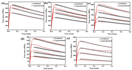
Figure 10.
Comparison between the predicted stresses by the modified Arrhenius model and the experimental ones: (a) 700 °C, (b) 750 °C, (c) 800 °C, (d) 850 °C, and (e) 900 °C.
- The ANN Model
ANN is a powerful tool that provides individuals an approach to bridge the complex connection between the input variables and output responses for any complex system [34]. In this section, an ANN model with a backpropagation (BP) algorithm was employed to describe the stress-strain relationship of SLM-manufactured Ti–6Al–4V in dynamic compression processes. Figure 11 displays the structure of a typical three-layer BP artificial neural network (BP-ANN). The input data consist of three variables such as strain, strain rate, and temperature. The output is flow stress. The hyperbolic sigmoid function is the transfer function in the hidden layer, and the linear function is the transfer function in the output layer. The gradient descent optimization algorithm is adapted to update the weights and biases. The Bayesian regularization algorithm is used to train the network. After several attempts, the number of neurons in the hidden layer was selected as 10 so that the network could perform best. A total of 285 experimental data were picked from a strain range of 0.05–0.4 in steps of 0.025. Before the network training, the input and output data were normalized according to the Equation (19) for more efficient training:
where, is the standardized input data, is the maximum experimental value, and is the minimum. Additionally, it is noteworthy here that 60% of input and output variables are selected randomly as training data, and the rest is used for testing. The outputs are converted into the original values by Equation (20):
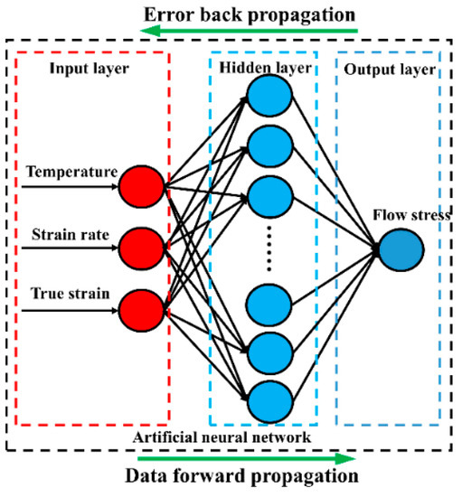
Figure 11.
Schematic diagram of a typical three-layer BP artificial neural network.
As shown in Figure 12, it could be found that the predicted stresses by the BP-ANN model are well consistent with the measured stresses. The value of the average absolute relative error between prediction and measurement is only about 0.7%.
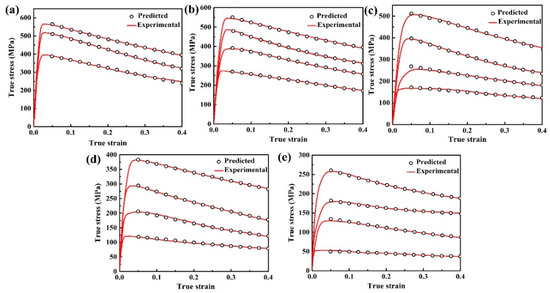
Figure 12.
Comparison between the prediction by the BP-ANN model and the measurement: (a) 700 °C, (b) 750 °C, (c) 800 °C, (d) 850 °C, and (e) 900 °C.
- Comparisons between the BP-ANN and the Modified Arrhenius Models
As shown in Table 5, the values of R for all the models are above 0.98 and the values of AARE are 7.6%, 4.0%, and 0.7% for the original Arrhenius model, the modified model, and the BP-ANN model, respectively. After modification, the relative error of the Arrhenius-type is reduced by 47%. Among these models, the ANN model has the highest accuracy. This is mainly because of its intelligent algorithm, which can approach the target value infinitely. With respect to the BP-ANN model, the modified Arrhenius-type model has a relatively low precision but definite physical significance, which considers the heat activated softening mechanism and gives out detailed expressions. In addition, for the stage where the strain should be less than 0.05, it can be regarded as the ideal plasticity and exhibits no obvious softening.
Table 5.
The calculated values of ARRE and R for the Arrhenius model and BP-ANN model.
Lastly, the proposed models were further cross-validated according to that in Mosleh et al. [35]. In each verification, one experimental curve was excluded from the model data. Three typical experimental curves were picked out as shown in Table 6. The deviation between the predicted and experimental values in the cross-validation was evaluated using Equation (21):
where is the maximum strain value in the model data. The comparison of experimental and predicted curves for No. 1 verification is depicted in Figure 13a. The deviations between the measurement and prediction for the proposed models in all the excluded conditions are shown in Figure 13b. After cross-validation, it could be clearly observed that the modified Arrhenius model has stronger predictability for the flow stress than the BP-ANN model in excluded conditions. The ANN could well fit and approach the model data. However, it requires a large amount of data to train the network for the accurate prediction of untested data.
Table 6.
The excluded conditions in the cross-validation.
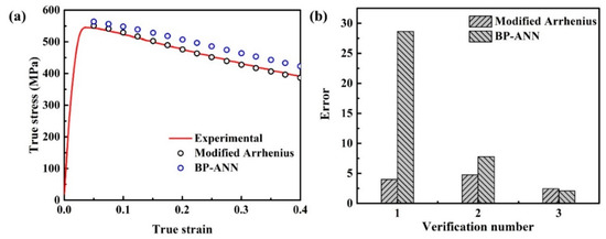
Figure 13.
(a) Comparison between the prediction by both models and measurement and (b) the deviations between the measured stress and the predicted stress in cross-validation.
4. Conclusions
The microstructure, mechanical properties, and stress-strain behavior of Ti–6Al–4V produced by SLM were investigated in the present work. Various models were attempted to predict the deformation behavior during the quasi-static process at room temperature and the dynamic process at high temperatures. Based on the above analysis, the following conclusion could be drawn:
- (1)
- The as-fabricated microstructure of Ti–6Al–4V alloy contains columnar grains and fine martensitic needles due to extremely fast cooling rates, resulting in higher strength and lower ductility at room temperature, compared to the as-cast and forged Ti–6Al–4V. The average yield and ultimate strength is as high as 1036–1187 MPa and about 1300 MPa, respectively. The average elongation to failure is 6.8–8.7% and the average reduction of area is 21.30–28.60%.
- (2)
- The room temperature quasi-static tensile behavior of the SLMed Ti–6Al–4V alloy exhibit the features of continuous yielding and unobvious work-hardening. During high-temperature dynamic compression, the flow stress quickly arrives at the peak value when the strain is small. The softening rate of flow stress varies with strain rates and temperatures.
- (3)
- The J–C model is suitable to forecast the quasi-static deformation behavior of SLMed Ti–6Al–4V at room temperature, but the model constants might rely on the specific process conditions because of the issue of building consistency.
- (4)
- The established modified Arrhenius and BP-ANN models could approach the stress-strain behavior during hot dynamic compression with enough precision. However, the established modified Arrhenius model is more predictive of the conditions out of the model data.
For the limited effective compression load of the thermal simulator Gleeble-1500, the hot compression in this paper was only performed at temperatures above 700 °C. The flow behavior of the SLMed Ti–6Al–4V alloy at temperatures below 700 °C will be further studied in future work using the thermal simulator Gleeble-3800. In addition, the anisotropy in compression behavior will be considered.
Author Contributions
P.T. and J.Z. performed the experiments; H.L., Q.H. and S.G. provided the tested samples; P.T. and Q.X. wrote the manuscript; and Q.X. revised the manuscript.
Funding
This work was supported by the National Program on Key Basic Research Project of China (No. 613281), National Natural Science Foundation of China (No. 51505451), Natural Science Foundation of Beijing (No. 3172042), and EMUSIC which is part of an EU-China collaboration and has received funding from the European Union’s Horizon 2020 research and innovation program under grant agreement No. 690725 and from MIIT under the program number MJ-2015-H-G-104.
Conflicts of Interest
The authors declare no conflict of interest.
References
- Tao, P.; Shao, H.; Ji, Z.; Nan, H.; Xu, Q. Numerical simulation for the investment casting process of a large-size titanium alloy thin-wall casing. Prog. Nat. Sci. 2018, 28, 520–528. [Google Scholar] [CrossRef]
- Banerjee, D.; Williams, J.C. Perspectives on titanium science and technology. Acta Mater. 2013, 61, 844–879. [Google Scholar] [CrossRef]
- Sallica-Leva, E.; Caram, R.; Jardini, A.L.; Fogagnolo, J.B. Ductility improvement due to martensite α′ decomposition in porous Ti–6Al–4V parts produced by selective laser melting for orthopedic implants. J. Mech. Behav. Biomed. Mater. 2016, 54, 149–158. [Google Scholar] [CrossRef] [PubMed]
- Chen, J.; Zhang, Z.; Chen, X.; Zhang, C.; Zhang, G.; Xu, Z. Design and manufacture of customized dental implants by using reverse engineering and selective laser melting technology. J. Prosthet. Dent. 2014, 112, 1088–1095. [Google Scholar] [CrossRef] [PubMed]
- Yan, C.; Hao, L.; Hussein, A.; Bubb, S.L.; Young, P.; Raymont, D. Evaluation of light-weight AlSi10Mg periodic cellular lattice structures fabricated via direct metal laser sintering. J. Mater. Process. Technol. 2014, 214, 856–864. [Google Scholar] [CrossRef]
- Herzog, D.; Seyda, V.; Wycisk, E.; Emmelmann, C. Additive manufacturing of metals. Acta Mater. 2016, 117, 371–392. [Google Scholar] [CrossRef]
- Sun, J.; Yang, Y.; Wang, D. Parametric optimization of selective laser melting for forming Ti6Al4V samples by Taguchi method. Opt. Laser Technol. 2013, 49, 118–124. [Google Scholar] [CrossRef]
- Yang, J.; Yu, H.; Yin, J.; Gao, M.; Wang, Z.; Zeng, X. Formation and control of martensite in Ti–6Al–4V alloy produced by selective laser melting. Mater. Des. 2016, 108, 308–318. [Google Scholar] [CrossRef]
- Simonelli, M.; Tse, Y.Y.; Tuck, C. Effect of the build orientation on the mechanical properties and fracture modes of SLM Ti–6Al–4V. Mater. Sci. Eng. A 2014, 616, 1–11. [Google Scholar] [CrossRef]
- Facchini, L.; Magalini, E.; Robotti, P.; Molinari, A.; Höges, S.; Wissenbach, K. Ductility of a Ti–6Al–4V alloy produced by selective laser melting of prealloyed powders. Rapid Prototyping J. 2010, 16, 450–459. [Google Scholar] [CrossRef]
- Edwards, P.; Ramulu, M. Fatigue performance evaluation of selective laser melted Ti–6Al–4V. Mater. Sci. Eng. A 2014, 598, 327–337. [Google Scholar] [CrossRef]
- Tao, P.; Li, H.-X.; Huang, B.-Y.; Hu, Q.-D.; Gong, S.-L.; Xu, Q.-Y. Tensile behavior of Ti–6Al–4V alloy fabricated by selective laser melting: Effects of microstructures and as-built surface quality. Chin. Foundry 2018, 15, 243–252. [Google Scholar] [CrossRef]
- Vilaro, T.; Colin, C.; Bartout, J.-D. As-fabricated and heat-treated microstructures of the Ti–6Al–4V alloy processed by selective laser melting. Metall. Mater. Trans. A 2011, 42, 3190–3199. [Google Scholar] [CrossRef]
- Kasperovich, G.; Hausmann, J. Improvement of fatigue resistance and ductility of TiAl6V4 processed by selective laser melting. J. Mater. Process. Technol. 2015, 220, 202–214. [Google Scholar] [CrossRef]
- Bagehorn, S.; Wehr, J.; Maier, H.J. Application of mechanical surface finishing processes for roughness reduction and fatigue improvement of additively manufactured Ti–6Al–4V parts. Int. J. Fatigue 2017, 102, 135–142. [Google Scholar] [CrossRef]
- Cheng, X.Y.; Li, S.J.; Murr, L.E.; Zhang, Z.B.; Hao, Y.L.; Yang, R.; Medina, F.; Wicker, R.B. Compression deformation behavior of Ti–6Al–4V alloy with cellular structures fabricated by electron beam melting. J. Mech. Behav. Biomed. Mater. 2012, 16, 153–162. [Google Scholar] [CrossRef] [PubMed]
- Gautam, R.; Idapalapati, S. Performance of strut-reinforced Kagome truss core structure under compression fabricated by selective laser melting. Mater. Des. 2019, 164, 107541. [Google Scholar] [CrossRef]
- Wang, Z.; Li, P. Characterisation and constitutive model of tensile properties of selective laser melted Ti–6Al–4V struts for microlattice structures. Mater. Sci. Eng. A 2018, 725, 350–358. [Google Scholar] [CrossRef]
- Baxter, C.; Cyr, E.; Odeshi, A.; Mohammadi, M. Constitutive models for the dynamic behaviour of direct metal laser sintered AlSi10Mg_200C under high strain rate shock loading. Mater. Sci. Eng. A 2018, 731, 296–308. [Google Scholar] [CrossRef]
- Lu, X.; Lin, X.; Chiumenti, M.; Cervera, M.; Li, J.; Ma, L.; Wei, L.; Hu, Y.; Huang, W. Finite element analysis and experimental validation of the thermomechanical behavior in laser solid forming of Ti–6Al–4V. Addit. Manuf. 2018, 21, 30–40. [Google Scholar] [CrossRef]
- Thijs, L.; Verhaeghe, F.; Craeghs, T.; Van Humbeeck, J.; Kruth, J.-P. A study of the microstructural evolution during selective laser melting of Ti–6Al–4V. Acta Mater. 2010, 58, 3303–3312. [Google Scholar] [CrossRef]
- Zhong, H.Z.; Zhang, X.Y.; Wang, S.X.; Gu, J.F. Examination of the twinning activity in additively manufactured Ti–6Al–4V. Mater. Des. 2018, 144, 14–24. [Google Scholar] [CrossRef]
- Åkerfeldt, P.; Antti, M.-L.; Pederson, R. Influence of microstructure on mechanical properties of laser metal wire-deposited Ti–6Al–4V. Mater. Sci. Eng. A 2016, 674, 428–437. [Google Scholar] [CrossRef]
- Li, P.-H.; Guo, W.-G.; Huang, W.-D.; Su, Y.; Lin, X.; Yuan, K.-B. Thermomechanical response of 3D laser-deposited Ti–6Al–4V alloy over a wide range of strain rates and temperatures. Mater. Sci. Eng. A 2015, 647, 34–42. [Google Scholar] [CrossRef]
- Matsumoto, H.; Bin, L.; Lee, S.-H.; Li, Y.; Ono, Y.; Chiba, A. Frequent Occurrence of Discontinuous Dynamic Recrystallization in Ti–6Al–4V Alloy with α′ Martensite Starting Microstructure. Metall. Mater. Trans. A 2013, 44, 3245–3260. [Google Scholar] [CrossRef]
- Mur, F.X.G.; Rodriguez, D.; Planell, J.A. Influence of tempering temperature and time on the α′-Ti–6Al–4V martensite. J. Alloys Compd. 1996, 234, 287–289. [Google Scholar]
- Zhang, Z.X.; Qu, S.J.; Feng, A.H.; Shen, J.; Chen, D.L. Hot deformation behavior of Ti–6Al–4V alloy: Effect of initial microstructure. J. Alloys Compd. 2017, 718, 170–181. [Google Scholar] [CrossRef]
- Lin, Y.C.; Chen, X.-M. A critical review of experimental results and constitutive descriptions for metals and alloys in hot working. Mater. Des. 2011, 32, 1733–1759. [Google Scholar] [CrossRef]
- Sellars, C.M.; McTegart, W.J. On the mechanism of hot deformation. Acta Metall. 1966, 14, 1136–1138. [Google Scholar] [CrossRef]
- Wang, J.; Zhao, G.; Chen, L.; Li, J. A comparative study of several constitutive models for powder metallurgy tungsten at elevated temperature. Mater. Des. 2016, 90, 91–100. [Google Scholar] [CrossRef]
- Li, J.; Li, F.; Cai, J.; Wang, R.; Yuan, Z.; Xue, F. Flow behavior modeling of the 7050 aluminum alloy at elevated temperatures considering the compensation of strain. Mater. Des. 2012, 42, 369–377. [Google Scholar] [CrossRef]
- Shafaat, M.A.; Omidvar, H.; Fallah, B. Prediction of hot compression flow curves of Ti–6Al–4V alloy in α + β phase region. Mater. Des. 2011, 32, 4689–4695. [Google Scholar] [CrossRef]
- Peng, X.; Guo, H.; Shi, Z.; Qin, C.; Zhao, Z. Constitutive equations for high temperature flow stress of TC4-DT alloy incorporating strain, strain rate and temperature. Mater. Des. 2013, 50, 198–206. [Google Scholar] [CrossRef]
- Wu, S.-W.; Zhou, X.-G.; Cao, G.-M.; Liu, Z.-Y.; Wang, G.-D. The improvement on constitutive modeling of Nb-Ti micro alloyed steel by using intelligent algorithms. Mater. Des. 2017, 116, 676–685. [Google Scholar] [CrossRef]
- Mosleh, A.; Mikhaylovskaya, A.; Kotov, A.; Pourcelot, T.; Aksenov, S.; Kwame, J.; Portnoy, V. Modelling of the superplastic deformation of the near-α titanium alloy (Ti-2.5 Al-1.8 Mn) using Arrhenius-type constitutive model and artificial neural network. Metals 2017, 7, 568. [Google Scholar] [CrossRef]


© 2019 by the authors. Licensee MDPI, Basel, Switzerland. This article is an open access article distributed under the terms and conditions of the Creative Commons Attribution (CC BY) license (http://creativecommons.org/licenses/by/4.0/).