Abstract
There is currently a need for an efficient numerical optimization strategy for the quality of friction stir welded (FSW) joints. However, due to the computational complexity of the multi-physics problem, process parameter optimization has been a goal that is out of reach of the current state-of-the-art simulation codes. In this work, we describe an advanced meshfree computational framework that can be used to determine numerically optimized process parameters while minimizing defects in the friction stir weld zone. The simulation code, SPHriction-3D, uses an innovative parallelization strategy on the graphics processing unit (GPU). This approach allows determination of optimal parameters faster than is possible with costly laboratory testing. The meshfree strategy is firstly outlined. Then, a novel metric is proposed that automatically evaluates the presence and severity of defects in the weld zone. Next, the code is validated against a set of experimental results for ½” AA6061-T6 butt joint FSW joints. Finally, the code is used to determine the optimal advancing speed and rpm while minimizing defect volume based on the proposed defect metric.
1. Introduction
The friction stir welding (FSW) process is quickly becoming the joining method of choice for aluminum alloys. The solid-state process is able to form high-fidelity welds at excellent throughput rates. Because of the solid-state nature of the method, many types of defects are avoided that are associated with melting and solidification in conventional fusion welding processes. Nevertheless, depending on the process parameters, FSW joints can have volumetric defects that are detrimental to the ultimate strength of the joint. Determining the FSW process parameters that will prevent defects is a difficult task—one that is typically performed using trial and error experimentation. These experiments are costly and time-consuming. Given the inherent complexity of the friction stir welding process, the determination of optimal process parameters is an important field of research. Many researchers [1,2,3,4,5,6,7] have worked on determining optimal process parameters. These groups have focused on optimizing joint strength via experimental work. The general conclusion from these groups is that the rotational and advancing speeds play the most important role in the final weld quality.
Tamjidi et al. [8] used multi-objective biogeography-based optimization to optimize the process parameters for dissimilar butt joints composed of AA6061-T6 and AA7075-T6. Their approach allowed them to find the optimal tool speed, tilt, and offset based on a series of experiments in the lab. De Filippis et al. [9] developed an artificial neural network (ANN) to determine optimal process parameters for a butt joint of AA5754-H111. They performed experiments to obtain joint quality based on defects, strength, and hardness. Their ANN model was able to determine optimal rotation and advancing speed with good precision for the heat-affected zone and the ultimate strength of the joint. Vijayan and Rao [10] used an adaptive neuro-fuzzy inference system (ANFIS) to determine optimal advancing speed, rpm, axial load, and pin profile in order to maximize the tensile properties of aluminum alloys. They compared ANFIS to response surface method (RSM) models and found that ANFIS provided improved robustness and accuracy for the prediction of joint strength. A drawback of using an experimental approach for optimization is that the model must be trained with experimental data, which means that the model would be valid for specific material combinations, tool geometry, and clamping setup. Another set of experiments would then be required if one of these fundamental parameters was varied.
Compared to experimental work, analytical and simulation-based predictions can be well-suited for a wide range of materials and geometries. Qian et al. [11] proposed an analytical model to optimize process parameters for defect-free welds. They imposed mass conservation and balanced material flow from ahead of the tool towards the rear of the tool. This allowed them to derive an analytical expression for tool rotation and advancing speed based on optimal process temperature. Fraser et al. [12] used a Monte-Carlo approach coupled with a finite difference solution of the heat diffusion equation to determine optimal process parameter based on an optimal temperature range. Their model was able to predict the optimal advancing speed. However, the thermal model is only well-suited for simple butt joint weld geometries. Chen et al. [13] used computational fluid dynamics (CFD) to predict process temperature and material flow. They developed a boundary shear stress model that they report better predicts material than a boundary velocity model. Carlone et al. [14] performed CFD modeling using the commercial code ANSYS CFX to simulate butt joint FSW of AA2024-T3. They were able to predict results such as material flow, grain size, and micro-hardness profiles. Buffa et al. [15,16] established a rigid-viscoplastic model of the FSW process in the commercial finite element code DEFORM-3D. They used the model to investigate the feasibility of joining Tailor welded blanks using the FSW process. They also used their approach [17] to predict residual stresses in AA6064-T4 butt joints with excellent precision. Recently, Paulo et al. [18] developed an innovative shell-based finite element simulation model of the FSW process. Using a shell element approach drastically reduces the calculation time and allows the user to analyze large welded structures in a reasonable time frame. The model is able to predict residual stresses, hardness, and distortion. A slight drawback is that their model cannot predict surface and internal volumetric defects, since the shell formation does not predict material movement through the thickness of the plates.
Clearly, there is room for improvement regarding the numerical simulation of FSW. Tutum and Hattel [19] provide a brief review of the challenges and the current state-of-the-art in the numerical simulation of FSW for optimization purposes. They note that one of the major challenges is to significantly reduce the computational time using advanced parallelization strategies. They suggest that the graphics processing units can be efficient resources for improving the performance of complex multi-physics simulation problems. As of yet, there has not been an efficient and robust 3D finite element method (FEM) approach that is able to simulate the material flow in a Lagrangian framework, and thus the defects during FSW. The main difficulty with FEM is related to the use of Gaussian quadrature to resolve the integral weak formulation. Quadrature essentially provides a link between the geometric and computational domains (mapping using isoparametric coordinates). As the finite elements undergo large deformation, the quadrature scheme breaks down (as measured by the determinant of the element Jacobian, ). The quadrature scheme used for the volume integration of a field variable, , for 3D finite elements is:
where are the weights over the n, m, and l integration points in the , , and isoparametric directions [20]. Equation (1) shows that as diverges away from 1.0, the volume integration becomes less precise. In FSW, the deformation is excessive, and in order to prevent breakdown of quadrature, it is necessary to re-mesh the problem domain. Schmicker [21] had good success with FEM adaptive re-meshing algorithms in 2D for the rotary friction welding process. Other researchers [16,22,23,24,25] have focused on coupled Eulerian–Lagrangian (CEL) and arbitrary Lagrangian–Eulerian (ALE) approaches. These methods have advantages over FEM with re-meshing when it comes to dealing with large deformation. However, they are not true Lagrangian approaches, which makes following the material history difficult. Because of this, quantification of material mixing is not feasible in either CEL or ALE.
Since the major issue with simulating large deformation processes is associated with the mesh, an innovative approach is to use a numerical method that does not require a mesh. Such an approach falls into the class of meshfree methods, whereby the set of partial differential equations describing the physics of FSW are solved at a set of material points. There is a vast array of meshfree methods available, as described by Liu et al. [26,27]. Some of the more popular meshfree methods are the local radial point interpolation method (LRPIM) [28,29], meshless local Petrov–Galerkin (MLPG) [30], finite point method (FPM) [31], as well as the smoothed particle hydrodynamics method (SPH) [32,33]. Fraser et al. [34,35,36,37,38,39,40,41,42,43] have recently developed an advanced meshfree framework on the graphics-processing unit (GPU) to simulate the entire FSW process. Their code—SPHriction-3D—is able to predict temperature, process forces/torques, internal and surface defects, tool wear, and residual stresses.
In this work, the meshfree formulation employed in SPHriction-3D is initially outlined. Following that, the code is validated against experimental results for temperature history and defect volume. Next, an automatic defect quantification metric is proposed, which is built on the idea that the material points physically move in the simulation owing to the Lagrangian framework of SPH. This means that a volumetric defect will be captured naturally during the simulation. From the simulation results, the process operating-window is mapped out by considering a maximum admissible defect size. Furthermore, the defect metric is used to form a response surface (RS) that is a function of tool rotation and advancing speed. A steepest descent algorithm is used to determine the optimal process parameters from the RS that minimize the volume of defects. This work presents the first use of a fully-coupled 3D thermo-mechanical numerical approach that minimizes defect volume. Because of the parallel framework on the GPU, the simulation code is able to predict optimal process parameters in an expedient manner, namely within one day, using a multi-GPU computer system as opposed to many weeks with a CPU implementation. The proposed numerical optimization framework is faster and more cost-effective than experiment-based process optimization.
2. Methodology
In the following section, an outline of the meshfree formation is provided, followed by a brief look at the implementation on the GPU. Then, a defect metric is introduced that can be used to numerically evaluate weld quality. Finally, the optimization strategy is outlined.
2.1. Meshfree Approach
The smoothed particle hydrodynamics method was originally developed for astrophysics applications by Gingold and Monaghan [32] as well as independently by Lucy [33]. SPH is a true meshfree method that does not require a background mesh. This is in contrast to global space meshfree methods that require a background mesh to perform the spatial integration.
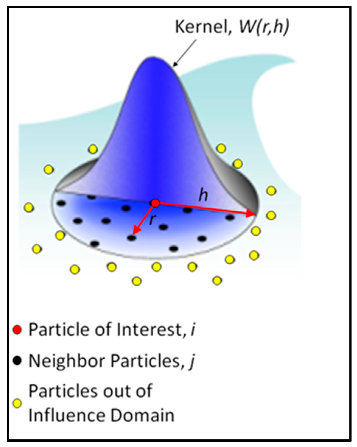
In SPH, spatial integration is performed directly at the nodes, as shown in Figure 1. To calculate the value of a field variable at an ith material point, a weighted sum is used over the jth neighboring material points within its influence domain. Mathematically, the discretized SPH approximation of a field variable, , at the spatial location, , of the ith material point is:
where is the smoothing length that determines the size of the influence domain of the th point on point . The material point mass and density is and , , and is an interpolation kernel, often referred to as the smoothing function. In this work, the smoothing function of Yang et al. [44] is used. The sum is taken over the total number () of material points within the influence domain of ; these are termed the neighbors of i. Using the SPH formalism, the gradient of a scalar and divergence of a vector are
and

Figure 1.
Interpolation in the smoothed particle hydrodynamics method (SPH). Reproduced from [36].
SPHriction-3D solves a set of continuum mechanics equations described by the conservation of mass, momentum, and energy (heat diffusion in this case). An abbreviated set of the partial differential field equations and their discretized counterparts using the SPH approach are listed in Table 1. A summary of the supporting equations and the associated nomenclature is provided in Table 2 and Table 3. Full details of the field equations and their SPH formulation can be found in [34,36,37,40,41,42,43].

Table 1.
Field equations and their SPH formulation.
Table 2.
Supporting equations.
Table 3.
Nomenclature.
The Fraser–Kiss–St-Georges (FKS) material model that was developed by Fraser et al. [36] is used here. This model provides an improved flow stress prediction for AA6061-T6 at high temperature and plastic strain levels compared to other commonly used material models such as Johnson–Cook (JC) [45]. The material model is a multiplicative combination of strain hardening, ; thermal softening, ; and strain rate stiffening, , of the form
The model accounts for the fact that strain rate stiffening is insignificant at room temperature, but becomes more important at high temperature in 6xxx-series aluminum alloys. This phenomenon is not present in the JC model that is very popular for FSW simulation. Furthermore, the model is more precise in the range of plastic strain typical of FSW. The JC model predicts an ever-increasing flow stress with increasing plastic strain, which is not realistic in typical aluminum alloys. The flow stress as a function of plastic strain and temperature is shown in Figure 2a and as a function of strain rate and temperature in Figure 2b.
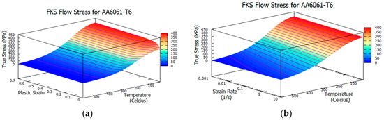
Figure 2.
Fraser–Kiss–St-Georges (FKS) flow stress model for AA6061-T6: (a) as a function of plastic strain and temperature; and (b) as a function of strain rate and temperature.
The set of ordinary differential equations that result from the SPH formulation are integrated in time with a second-order explicit time stepping algorithm that is outlined in detail in [36]. The mechanical and thermal timestep criteria to assure stability are:
Typically, the critical timestep for the thermal problem is one or two orders of magnitude greater than that of the mechanical problem. However, we have found that improved results are obtained by performing consistent temporal integration of the thermal and mechanical problems. This can be explained by the rapidly changing contact condition as the tool rotates and the associated heat generation due to friction.
Plastic deformation is accounted for by using the radial return algorithm, where the body is first assumed to deform elastically, and then a check is performed to see if the calculated stress surpasses the yield. If the material has yielded, the stress is projected back onto the yield surface. Due to the small timestep required for stability, the plastic strain increment can be found by performing a Taylor series expansion with linearization from the current timestep [46].
Considering the difference in material stiffness between the tool and the workpieces, the support base, clamps, and tool can be modeled with rigid finite elements. On the other hand, the large deformation in the workpieces requires the use of the SPH material points. Thermal-mechanical contact between SPH and FEM is accomplished with a penalty based method that “pushes” the ith material points out of the jth FEM along its surface normal vector, , of the contacted FEM. The developed contact force in the normal direction is then
where and are the penetration and the penetration rate. The contact stiffness, , and the damping, , is given by
The force due to friction is based on a modified Coulomb law where the tangential force that acts on the ith material point will be
A tangential normal vector, , is found by normalizing the projection of the relative velocity between the ith material point and the contact point on the jth finite element onto the plane that passes through the nodes of the finite element. For the simulations reported here, a constant value of 0.5 is used for the coefficient of friction, . The contact area is denoted by , and is assumed to be a square patch with sides equal to the average spacing, , of the ith material point.
2.2. Parallelization on the GPU
Simulation of all the phases of the friction stir welding process within a multi-physics framework is computationally expensive. To achieve reasonable simulation times, the highly non-linear thermo-mechanical problem must be solved using an advanced parallelization strategy. SPHriction-3D has been developed to run on NVIDIA GPUs using the CUDA Fortran programming language (see Ruetsch and Fatica [47]).
The parallelization strategy used in the code is to assign each material point to a thread on the GPU (similar to a thread on a CPU). The summations in the SPH form are computed on each thread, which is an efficient use of the GPU architecture. Although the clock speed of the thread processors on the GPU are slower than on the CPU, the sheer number of threads and the rate at which they are able to change tasks (context switching) makes the GPU the ideal platform to parallelize the SPH code. The simulation is initialized (all model data, mesh, and material point information) on the CPU. The information is then transferred to the GPU and resides there for the remainder of the simulation. This is only possible in a code that has been entirely programmed to run on the GPU, thus minimizing costly data transfer back and forth from the CPU and the GPU. Various test cases have been run in SPHriction-3D and compared to an equivalent commercial SPH code running on an Intel i7-3630QM processor (Intel Corporation, Santa Clara, CA, USA). The results from these tests have shown that the GPU code is over 20 times faster. Models that previously required weeks of calculation time can now to run in a few hours. This improvement in calculation time makes the concept of finding optimal process parameters numerically a viable option.
2.3. Defect Metric
In order to evaluate the effect of different process parameters on the formation of defects in the simulation, a non-dimensional metric should be established. Because of the Lagrangian nature of the simulation code, internal and external free surface areas can be determined and used to evaluate the presence of defects. The metric will compare the pre-weld surface area, , to that in the post-weld, , based on
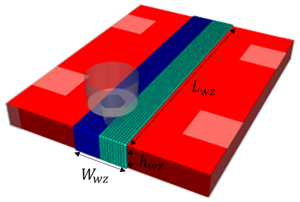
The pre-weld area is selected to include the region within the weld zone as shown in Figure 3. The area is calculated from
which includes an approximation for the surface area associated with the hole created by the pin of length and radius . The material points that belong to the free surface are determined via
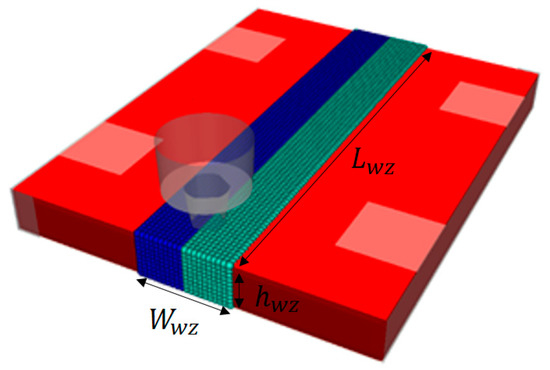
Figure 3.
Measuring zone for initial pre-weld surface area.
The post-weld area is determined by counting the number of material points that are surface nodes, , in the measuring zone and multiplying by the surface area of the material point (a square patch with side of ):
The number of surface nodes is found by looping over all the elements and counting the elements that are tagged . In this sense, a perfect weld with no defects will have a value of ; this would correspond to a case where . As the simulation progresses, the defect metric will naturally fall below 1.0. The actual surface area associated with the defects can be found from
It is important to note that contains contributions from internal volumetric defects as well as the increase in surface area on the surface of the weld in the weld track.
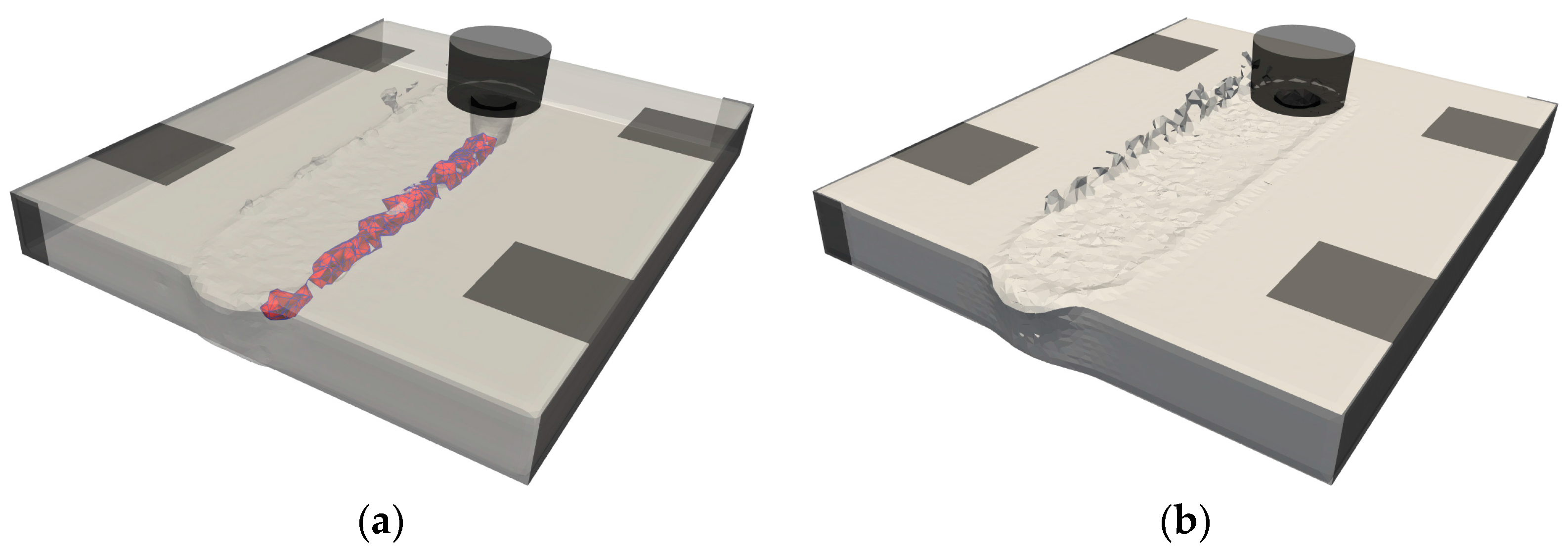
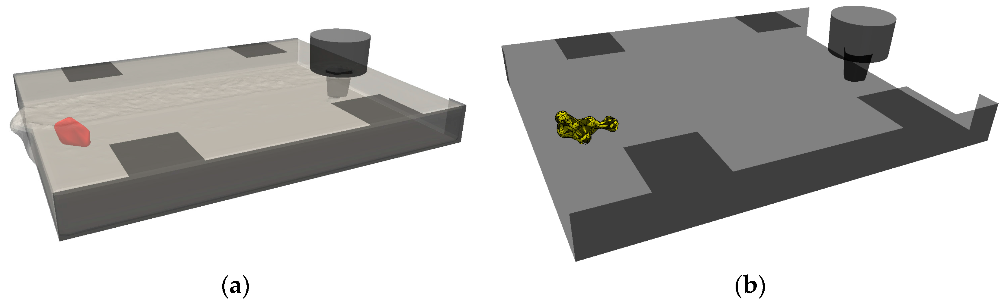
Once the set of material points that belongs to the free surface is found, a triangulation algorithm is used to create a smooth surface. An example of the triangulated surface for the internal defects is shown in Figure 4a, and for the surface defects (flash and weld track striations) in Figure 4b. Very hot welds with low weld pitches will tend to produce more flash and weld track striations than a cold weld. For this reason, including the area associated with the weld surface in the metric is an important part of our approach. If this area were to be excluded from the calculation, welds with low weld pitches that have no or very little internal volume defects would score better than cold welds with small-to-medium-sized internal defects (voids and worm-holes). The proposed defect metric is a powerful tool to numerically determine the process operating-window as well as the optimal process parameters.

Figure 4.
(a) shows the triangulated internal defects (in red) and (b) shows the flash formation and increased surface area in the weld track for a case with 500 rpm and 102 mm/min advance.
2.4. Optimization Approach
Finding the set of process parameters that minimizes the probability of defects in the weld zone could be accomplished using a variety of different optimization strategies. The approach chosen should be implementable within the framework of the numerical code in order to provide optimized results without the need for visual inspection of the simulation results. The true beauty of using the Lagrangian meshfree code is that all calculations regarding defect size and location are handled automatically in the code. The code simply needs to run through a batch of process parameters and to store the associated defect metric for the different combinations of tool rotation and advancing speed.
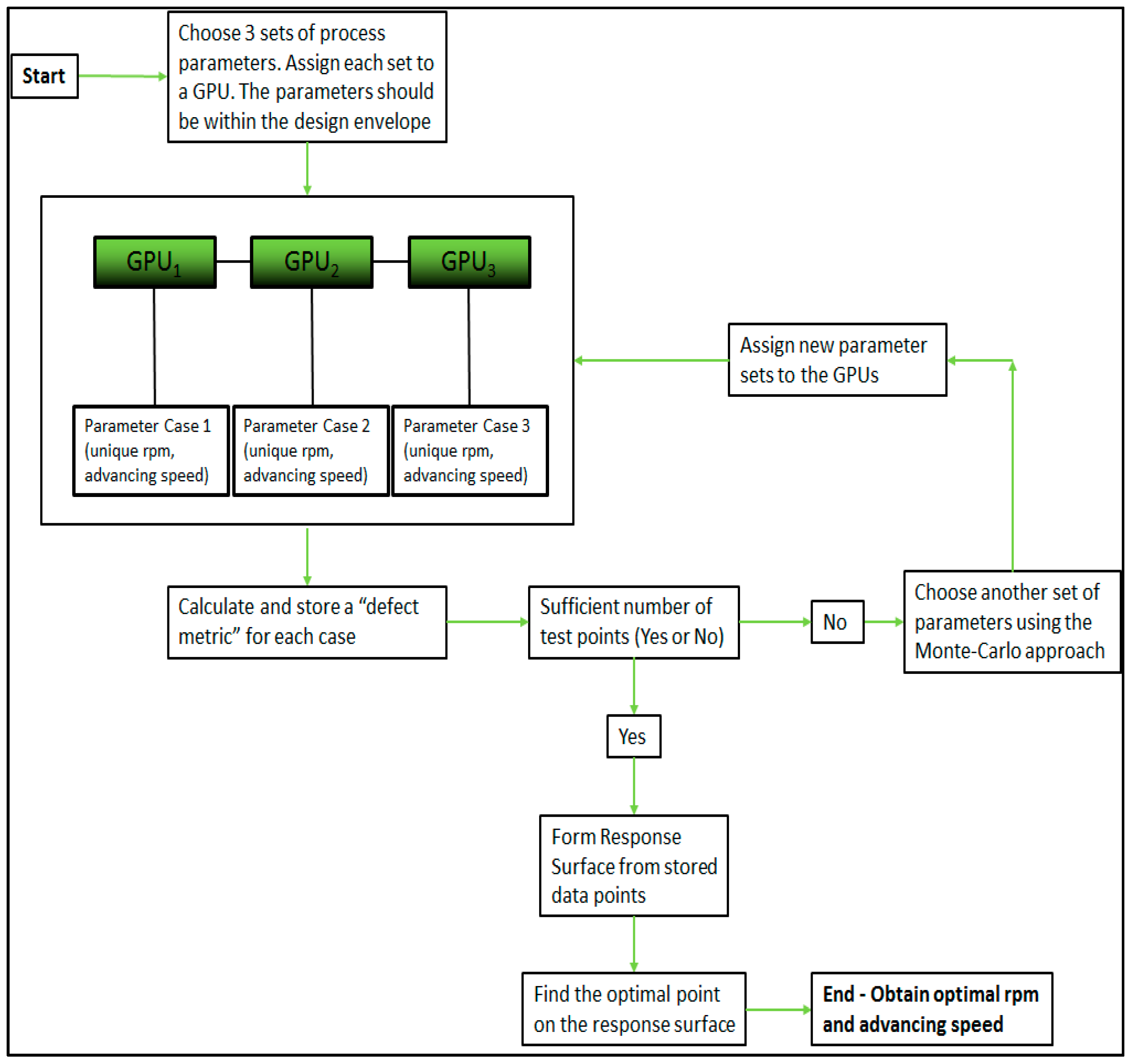
Because the code runs on the GPU, a relatively inexpensive computer with four GPUs can simultaneously run four individual simulations. Once a simulation has finished computing a case, the GPU will be available to run another simulation. As soon as enough simulations have been performed to provide an adequate amount of data sets, the optimization routine is then called. In this work, we use a second-order polynomial surface function with eight coefficients to form a response surface. The number of simulations should be at least greater than the number of coefficients to be found. Evidently, more data sets are beneficial to ensure the highest level of accuracy for the response surface. However, running an extensive set of simulations will lead to longer calculation times. Fifteen different parameter sets (shown in Table 4) have been used to form the response surface. A summary of the optimization procedure with a three-GPU system is shown in Figure 5. In our approach, since a simulation model is run on one individual GPU, the performance will increase linearly when increasing the number of GPUs. That is to say, if you run one simulation on the GPU and it takes two hours, running four simulations on four GPUs will also take two hours, leading to a performance increase of four times. The linear improvement in performance is possible since there is no communication between the individual GPUs. This approach can be used as long as the data from the individual simulation models can fit onto the GPU’s memory. Current state of the art consumer GPUs (for example the NVIDIA GTX 1080 Ti, Nvidia Corporation, Santa Clara, CA, USA) have up to 11 GB of onboard memory, which allows us to simulate meshfree thermo-mechanical models with over two million material points. The memory model currently employed in SPHriction-3D leads to ~5.5 KB storage requirements per material point. The high storage requirements help to improve the calculation efficiency of the code by saving valuable neighbor information, smoothing, and derivative values.
Table 4.
Process parameter sets for optimization.
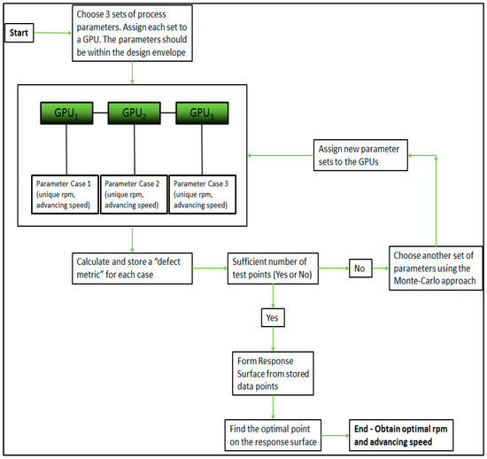
Figure 5.
Optimization procedure with three graphics-processing units (GPUs).
Our approach leads to a powerful means of numerically determining optimal process parameters within a 24-h period without the need to perform time-consuming and costly experiments.
3. Validation of the Numerical Model
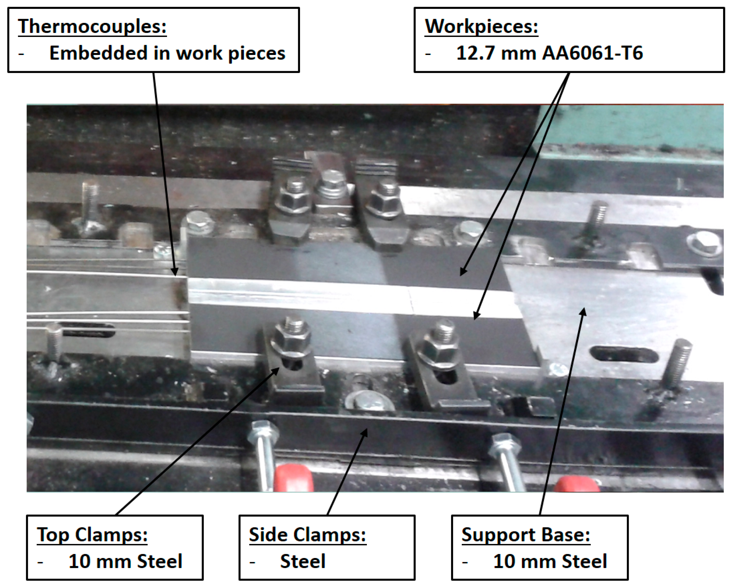
Validation of the material point temperatures as well as defect size and location is required before the simulation code can be used to determine optimal parameters. In this section, temperature history, temperature contours, and defect size will be compared with experimental results. The experimental setup for the butt joint weld of two ½” AA6061-T6 plates is shown in Figure 6. The surface of the workpieces was painted flat black with a high-temperature paint in order to obtain quality images with an infrared camera. The clamping system applied pressure to hold the plates together as well as hold them down on the support base. The material properties used in the simulations for the workpieces and the tool are listed in Table 5, Table 6 and Table 7.
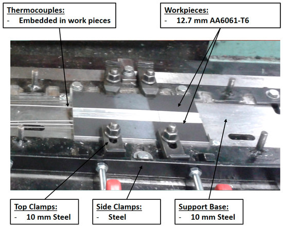
Figure 6.
Experimental setup.
Table 5.
FKS material model constants.
Table 6.
Work piece thermophysical properties [48].
Table 7.
Tool thermophysical properties.
The tool used was a tri-flute design with a shoulder diameter of 21.6 mm, upper pin diameter of 11 mm, lower pin diameter of 8.4 mm, and a pin length of 10.8 mm. Three cases were simulated and compared to experimental results. The cases are:
- 800 rpm, 305 mm/min–0.38 weld pitch
- 800 rpm, 660 mm/min–0.83 weld pitch
- 800 rpm, 1069 mm/min–1.34 weld pitch
The validation case parameters were selected to provide a large variation of weld pitches. We will show that the simulation model was able to predict temperature and defect with errors under 10%, thus confirming the robustness of our approach. In Section 4.1, validation of the calculated optimal process parameters will be provided by comparing the predicted defects from simulation to those measured experimentally.
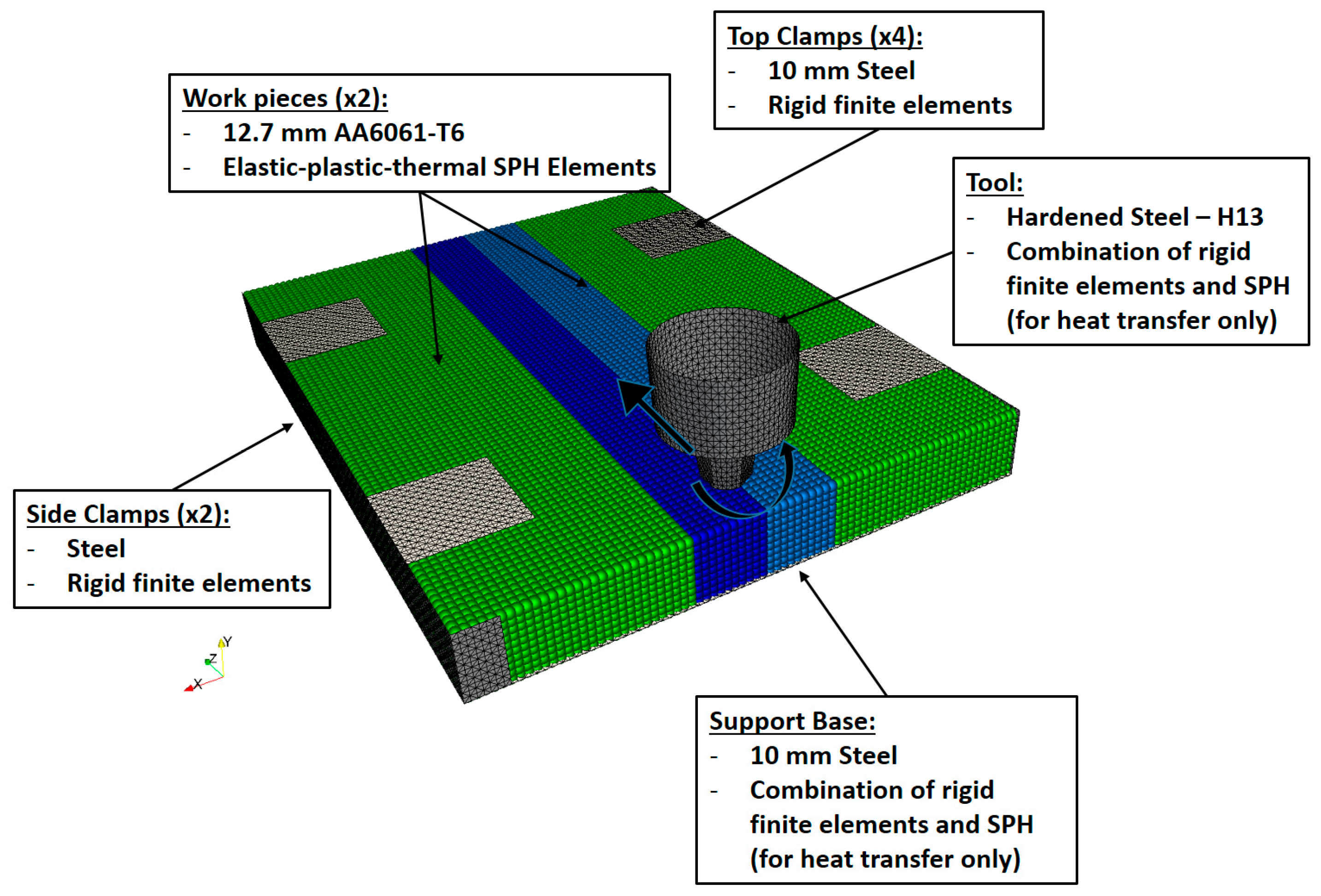
All three cases used a plunge speed of 38 mm/min and a dwell time of five seconds. The simulation model is shown in Figure 7. The material point spacing was , which provides 10 points through the thickness of the workpieces. Based on the stability criterion, the time step size was s, with timestep factor, CFL = 0.7. The simulation model for the workpieces was 100 mm wide by 150 mm long by 12.7 mm thick. The length of the workpieces was selected to provide enough distance along the length of the weld to attain a state where the change in system energy remained stable. A full transient calculation was performed wherein the tool starts entirely disengaged from the workpieces, then plunges, dwells, advances, and retreats. A good prediction of defects and other material history is only possible when the full sequence of welding events is modeled.

Figure 7.
Simulation model setup.
3.1. Temperature History and Contour Validation
Thermocouples were embedded into the workpieces to measure the temperature history in the advancing phase. The thermocouples were used to validate the calculated temperatures in the simulation. The location of the thermocouples is shown in Figure 8a. The temperature history was compared for the 0.38 weld pitch case in Figure 8b, the 0.83 weld pitch case in Figure 8c, and the 1.34 weld pitch case in Figure 8d. We can see good correlation among the temperature histories. As the weld-pitch increased, the temperatures measured in the experiments and calculated in the simulations decreased. This is an expected result, since less heat is generated with increasing weld pitch. The peak measured/calculated temperature was 281/269 (4.3% error), 208/210 (1.0% error), and 171/184 (4.0% error) for the 0.38, 0.83, and 1.34 weld pitch cases, respectively. Note that the temperature histories end shortly after the peak temperature was obtained. This is because the simulations terminated at the end of the advancing phase and did not include the cooling phase. In future work, we plan to extend the simulations into the cooling stage to determine residual stresses and distortion; however, for the current work, prediction of the peak advancing temperature was sufficient.
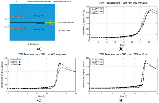
Figure 8.
(a) Location of thermocouples for temperature history. Temperature history comparison between experiment and simulation for 800 rpm with: (b) 305 mm/min, (c) 660 mm/min, and (d) 1069 mm/min.
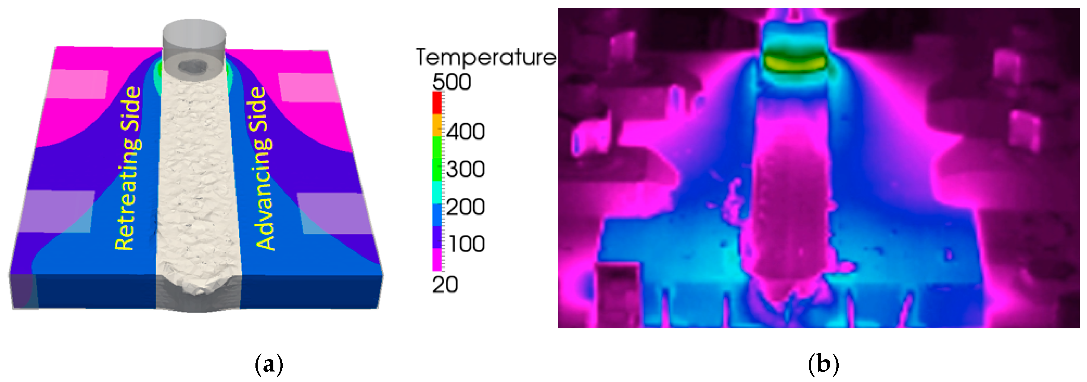
The temperature contours at the end of the simulation in Figure 9a are compared to experiment in Figure 9b by using an infrared thermal camera. The camera requires a surface with uniform reflectivity to give a good result, which was obtained by painting the top surface of the plates a flat black. The region where the FSW tool will pass could not be painted, since this would adversely affect friction at the tool–work piece interface. For this reason, the temperature contours are not shown in the weld track. Again, good correlation between simulation and experiment was found. The highest temperature was closest to the FSW tool and decreased further away from the tool. The plunge and dwell parameters led to high temperatures at the start of the weld. This is obvious in Figure 9a,b due to the shape of the temperature contours at the start of the weld.
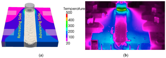
Figure 9.
Comparison of temperature contours at the end of the advancing phase between the (a) numerical and (b) experimental results for 800 rpm with 1069 mm/min advance speed.
3.2. Defect Validation
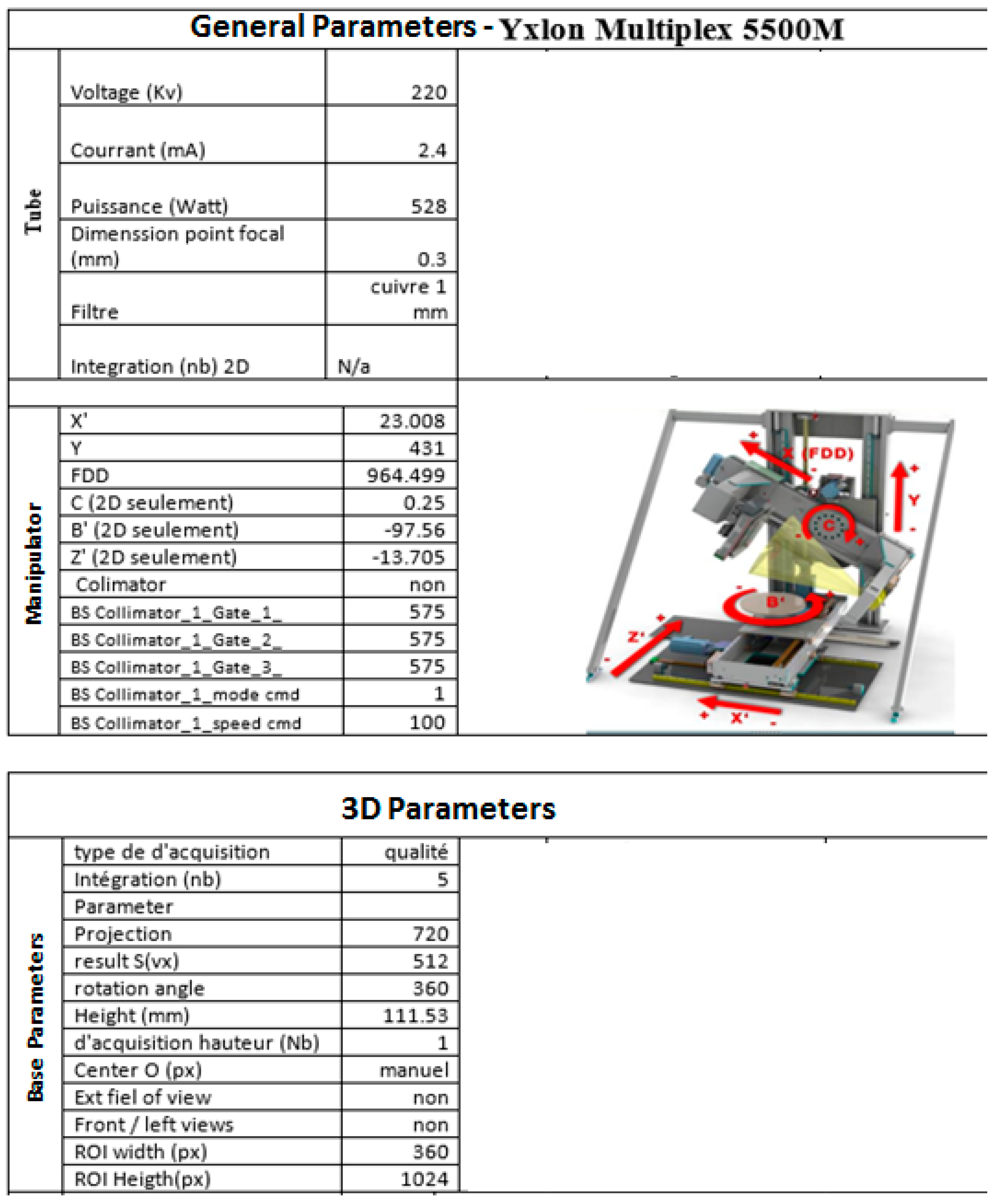
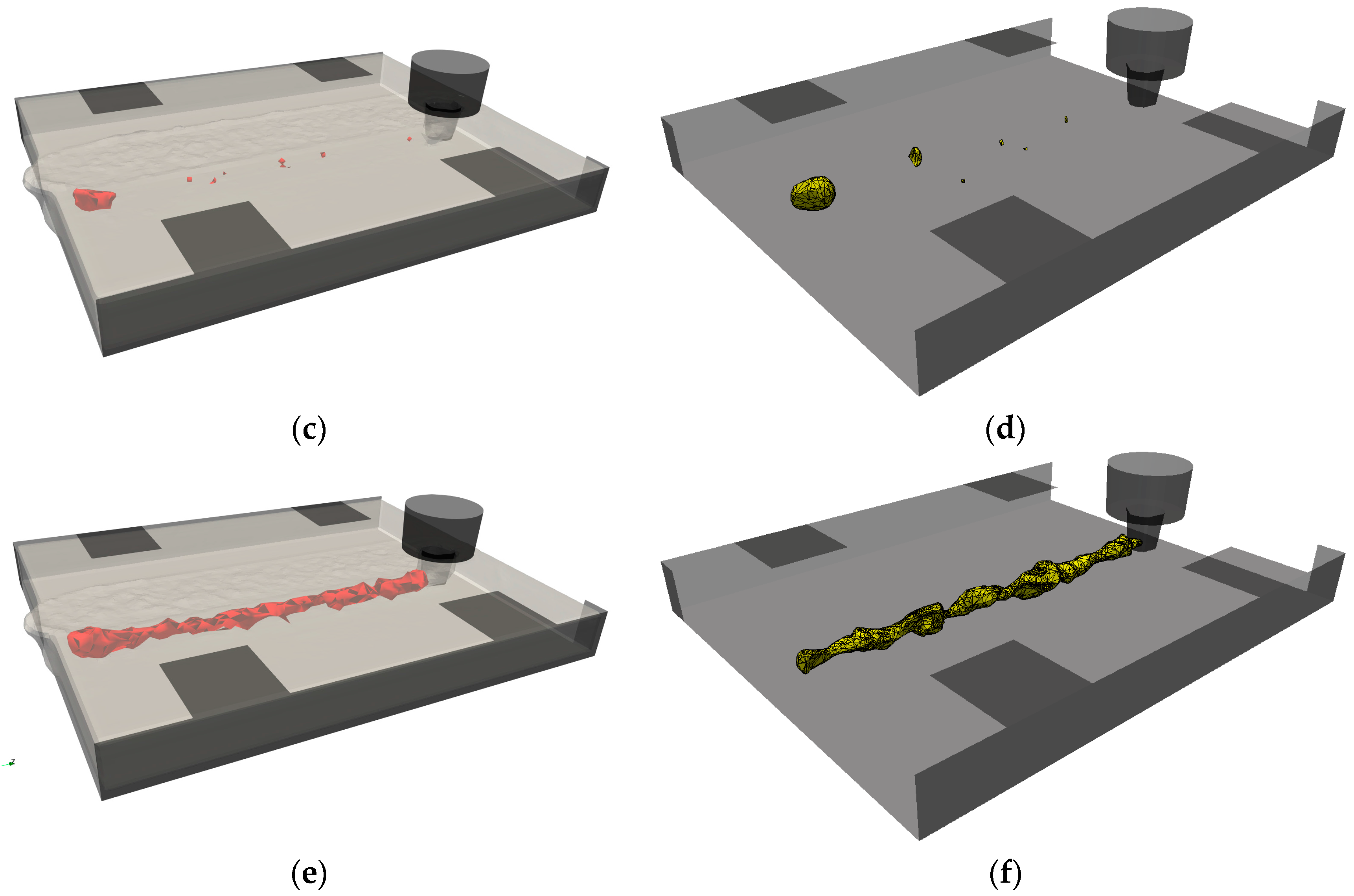
The defects present in the welds performed in the experiment were evaluated using X-ray tomographic imaging (X-ray herein) with an advanced void detection algorithm. This method is non-destructive and provides an interesting means of measuring the location and size of volumetric defects in a friction stir welded joint. Certainly, the X-ray technique is perfectly suited for research work where the weld samples are small enough to fit into the confines of the X-ray enclosure. Such an approach would not be possible for industrial welds of parts with large dimensions. The X-ray system’s void detection algorithm was calibrated using an aluminum block with cavities of known dimensions and location. The parameters used to perform the X-ray images are provided in Appendix A. A comparison between the predicted defects from simulation and those measured from the experiments for the 0.38 weld pitch case is shown in Figure 10a,b. The defects were mainly at the start of the weld in the plunge/dwell zone; however, small defects were predicted and measured along the weld as well. The 0.83 weld pitch case is shown in Figure 10c,d. This case showed defects in the plunge/zone only, and no defects were present elsewhere in the weld. The third validation case, with a weld pitch of 1.34, is shown in Figure 10e,f; here extensive defects were predicted and measured throughout the entire weld as well as in the plunge/dwell region. The void detection algorithm employed by the X-ray system evaluates the local density at discrete points throughout the sample. When a region with decreased density is found, the algorithm flags the region as a possible defect and associates a probability. The algorithm returns the location and size of the defect by assuming that the defect is a spheroid. In [36], the surface area calculated from the X-ray void algorithm was used directly to compare to the simulation results, which led to an inaccurate prediction of the defect surface area. In this work, we have used the location of the center of the spheroids and their radii to perform surface triangulation in order to get a measurement of the volume of the internal defects. The procedure is as follows:
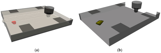
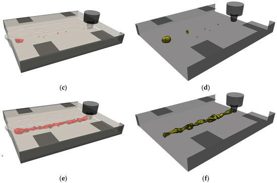
Figure 10.
Comparison of predicted and measured defects at the end of the advancing phase: (a,b) show 0.38 weld pitch, (c,d) show 0.84 weld pitch, (e,f) show 1.34 weld pitch.
- Create set of points from X-ray results with x, y, z position and defect radius
- Re-sample the data to add more points on the surface of each spheroid
- Find the nearest neighbors for the re-sampled data
- Calculate the normal vectors and find the free surface points using Equation (11)
- Perform Delaunay tessellation to discretize the defect domain with tetrahedral elements
- Calculate the volume of each of the tetrahedrons and determine the overall defect volume (sum of individual element volumes)
In this section, the volume predicted in the numerical simulations only includes the internal defects; the increase in surface area in the weld track due to the semi-circular striations is excluded. This is done because the X-ray system is not able to determine such an increase in surface area. This approach is different from what was reported in [36]. A comparison of the predicted and measured defect volumes is provided in Table 8. The volume was greatest for the case with a weld pitch of 1.34 and least for the 0.83 weld pitch case.
Table 8.
Defect volume comparison between simulation and experiment.
Typically, in the FSW process, the probability of defects being present in the weld increases as the weld pitch increases. The simulation models accurately predicted this trend and showed a volumetric defect prediction error in the range of 6–10%.
4. Results
Once the simulation method was validated, it could be used to determine optimal process parameters. The first step in the optimization process is to run enough simulations to have a large enough data set to for a response surface. A total of 15 simulations were run in SPHriction-3D with the parameters provided in Table 4.
4.1. Optimal Process Parameters
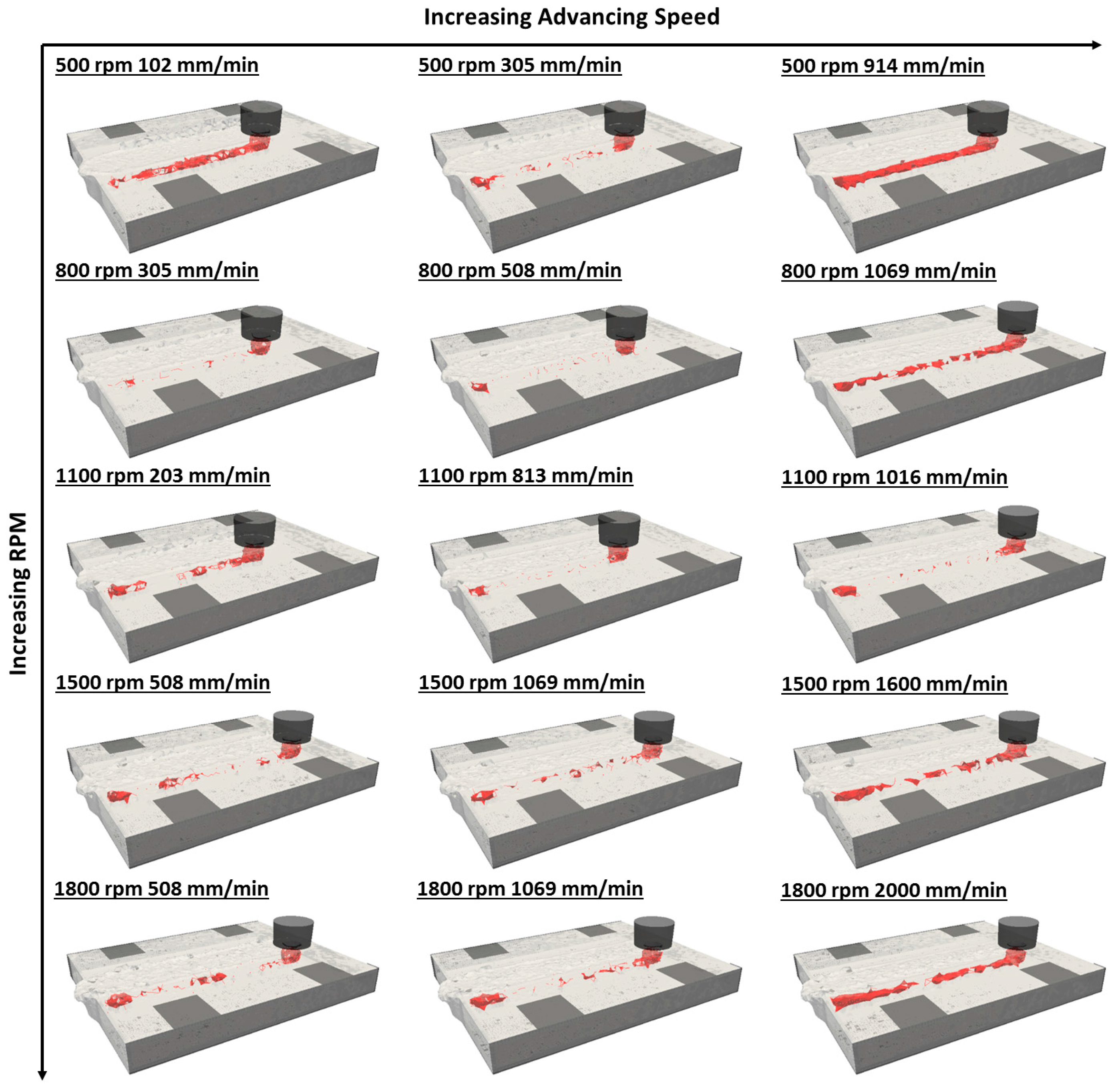
At the end of each of the simulations, the final value of the defect metric was recorded and stored for the optimization algorithm. The predicted internal defects for the 15 cases are shown in Figure 11. The images are arranged for increasing advancing speed from left to right and increasing rpm from the top to the bottom. From inspection of the results, we can see that the defects were minimized when the weld pitch was in the range of 0.5–0.8.
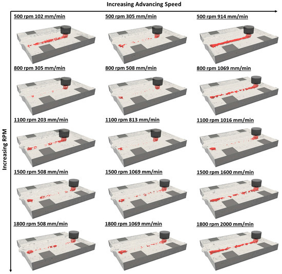
Figure 11.
Predicted defects for the 15 cases.
The data sets can now be used to form a response surface that characterizes the defect metric as a function of rpm () and advancing speed (). The function is of the general form
where the , , and coefficients are found from linear least squares regression analysis. The coefficients were , , , , , , , and . The R-squared value from the regression analysis was . The response surface is shown in Figure 12.
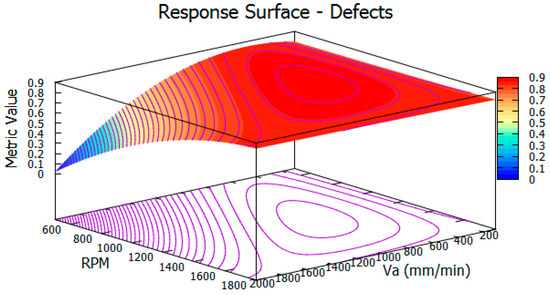
Figure 12.
Defect response surface.
The response surface shows that the weld quality decreases drastically as the weld pitch increases above 0.8, and decreases slightly for weld pitches below 0.5. Physically speaking, the welds with a pitch below 0.5 tend to exhibit surface defects such as galling due to overheating as well as excess flash along the retreating side of the weld. Welds with a pitch of over 0.8 tend to have internal defects such as worm-holes, voids, and incomplete welds. More detail on defect classification and detections is available from [49,50,51,52,53]. Inspection of the response surface suggests that the optimal process parameters that will minimize the defects will be located at the apex of the surface. To find the exact value of the rpm, , and the advancing speed, , we want to maximize the value of the defect metric, . To accomplish the aforementioned optimization, the problem to be solved is then:
| Maximize: | |
| Subject to (constraints): |
The lower bound constraints were selected to eliminate the process parameters that would lead to slow and costly welds. The upper bound constraints represent the limitation of the welding machinery. Certainly, the choice of constraints will be dependent upon settings specific to the industry as well as on factors relating to process productivity. The maximum point on the response surface is found by solving simultaneously the two following equations:
A series of results can be found by solving the set of equations. However, there is only one solution that satisfies the constraints. The optimal process parameters, and , are listed in Table 9.
Table 9.
Parameters that minimize defects.
To ensure that a local maximum has been found, the positive/negative definite of the Hessian matrix, , can be checked by:
Since the Hessian matrix is negative definite, a local maximum has been found.
In order to validate the simulation model’s ability to determine the optimal parameters, a simulation was run at and . The results of the simulation were compared to the defect reconstructed from the experimental X-ray images in Figure 13. The simulation predicted defects at the plunge/dwell zone only, which is in good agreement with the experimental results. A comparison of the predicted and measured defect volumes at the optimal process parameters is given in Table 10. The simulation predicted marginally less defect volume (9.7% precision error) than was measured from the experiment. The excellent correlation between the predicted and the measured defect volume at the optimal process parameters further validates the proposed optimization method and shows the robustness of our method.

Figure 13.
Comparison of predicted and measured defects at the end of the advancing phase for and : (a) simulation (b) experiment.
Table 10.
Comparison of predicted and experiment defect volume at optimal process parameters.
4.2. Process Window
Determination of the process window for friction stir welding is possible using a number of techniques. A popular approach is to perform a series of welds in the lab with various parameters, and then attempt to draw a curve that separates the good weld parameters from the poor ones. This method is also possible using numerical simulation, whereby the tests in the lab are substituted by numerical simulations. One of the drawbacks of this approach is that the choice of curve location and form to define the process window can be difficult.
Another approach is to use the results from the response surface to implicitly choose the shape of the curve that defines the process window. To accomplish this, it is necessary to first re-arrange the equation defining the response surface to obtain the advancing speed as a function of the rpm. This is akin to finding a level-set (iso-contour) of the response surface for a specific value that we will call . The parametric level set is defined by:
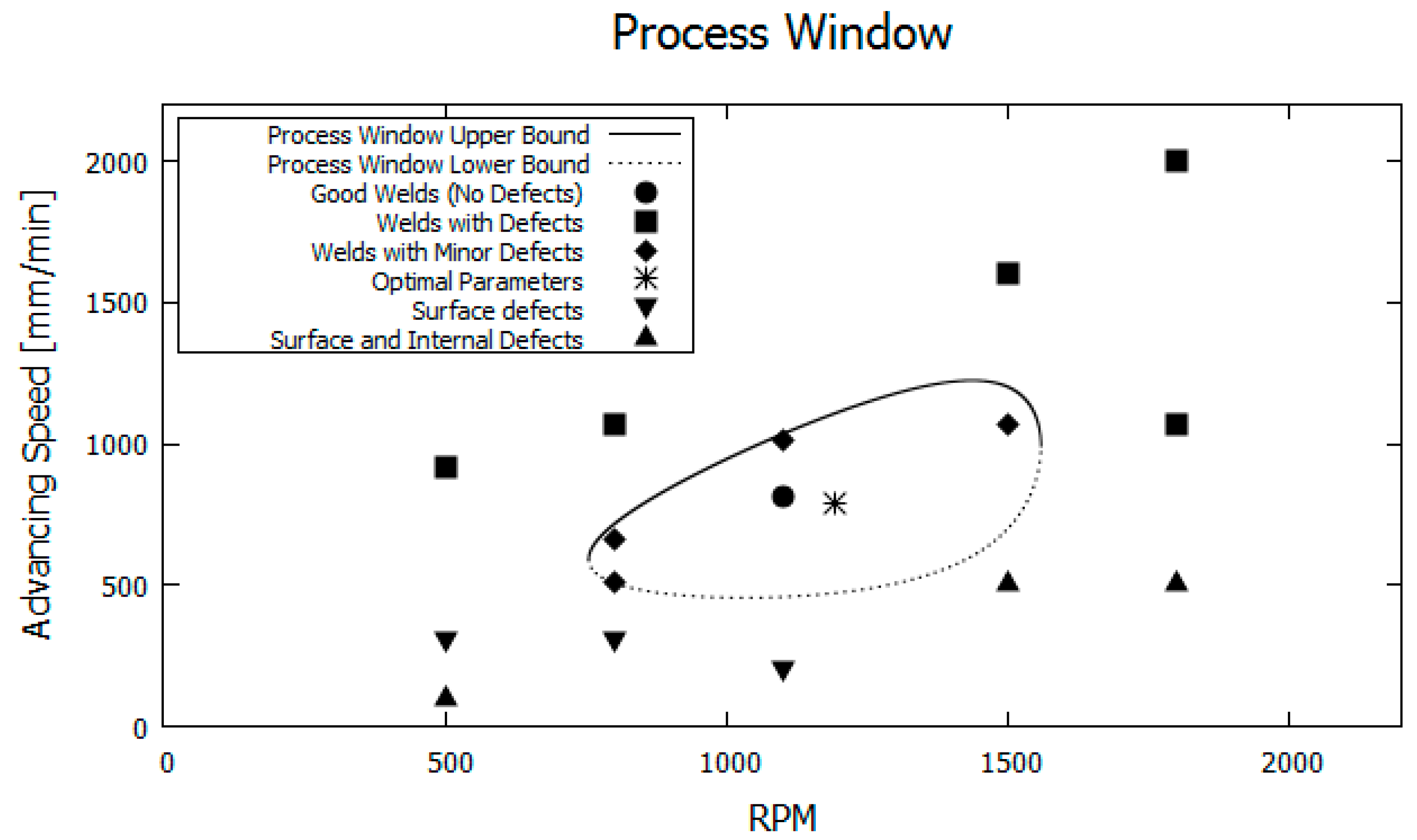
The choice of the value of will evidently change the size of the process window. For the FSW setup in this work, was varied until the process window encompassed the simulation points without defects and so that the boundary of the window was close to the welds with minor defects. Performing this procedure, the value determined for was 0.872. The resulting process window is shown in Figure 14. The welds in the graph are classified according to the following:
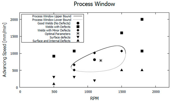
Figure 14.
Process window.
- Good welds (shown with ● on plot)—No defects are present in the advancing region of the weld. Defects in the plunge and retraction zone are permissible;
- Welds with minor defects (shown with ◆ on plot)—Minor internal defects are present. The extent of the defects is not to a point that the weld would necessarily be rejected;
- Welds with defects (shown with ■ on plot)—Welds that have extensive internal defects and would be rejected outright. Defects of this type would be voids, worm-holes, and incomplete welds;
- Welds with surface defects (shown with ▼ on plot)—These welds are typically very hot, leading to surface galling, tearing, hot cracking, and excessive flash. These welds would likely be rejected;
- Welds with surface and internal defects (shown with ▲ on plot)—These welds have significant internal defects as well as surface defects.
As previously mentioned, inspection of the simulation and experimental results suggests that weld pitched in the range of 0.5 to 0.8 led to satisfactory welds. This range of weld pitches is well captured in the process window.
5. Conclusions and Discussion
In this work, an efficient numerical approach was presented to determine optimal process parameters that minimize the presence of defects in a friction stir welded joint. The simulation models of the FSW process were calculated using an advanced meshfree coupled thermo-mechanical code on the GPU. The efficiency of the code allows determination of optimal process parameters within a few hours—a feat that was not previously possible when attempting to optimize using a multi-physics simulation approach.
The major developments presented are:
- Large-deformation Lagrangian solid mechanics formulation;
- Fully transient simulation of all phases of the FSW process;
- Meshfree method able to predict surface and internal defects;
- New material model for AA6061-T6;
- Defect metric that allows for automatic, on the fly, evaluation of defects in a FSW simulation model;
- Response surface methodology to determine optimal process parameters
- Implicit determination of the process window shape from simulation results
- Robust and efficient parallelization strategy.
The simulation code was validated in terms of temperature history and defects for three different parameter sets. The model results correlated excellently with the experimental data. The error associated with the prediction of the peak temperature during the advancing phase at a location in the work piece was found to be less than 4.3%, whereas the predicted defect volume error was under 10.1%. The location and appearance of the defects also corresponded well with the experimental results. By using a fully transient solution procedure along with a meshfree Lagrangian method, the intermittence and variability of the defects was also well captured.
The presented numerical simulation approach is a powerful design tool that allows the user to quickly determine the optimal process parameters for the FSW process. Since the actual process window is highly dependent on the FSW setup, tool shape, and operating conditions, only a highly sophisticated simulation model is sufficient to optimize the process. The presented method is able to take into account important aspects such as the support base material, clamping arrangement, as well as the features on the FSW tool. As such, the technique can be used to circumvent the need to perform time-consuming and costly testing in the laboratory or using production machinery. Ultimately, this leads to increased weld productivity and efficiency.
Acknowledgments
The authors would like to thank NVIDIA for donating GPUs used to perform the simulations. We would also like to thank the Portland Group (PGI) for having generously provided a license for PGI Visual Fortran (PVF) with CUDA Fortran. The project is supported in part by funding from FQRNT, CQRDA, GRIPS, REGAL, RTA, and CURAL. The authors would also like to the National Research Council of Canada (NRC) for providing the X-ray equipment and results.
Author Contributions
Kirk Fraser developed the simulation code, performed the experiments, and built the simulation models. Kirk Fraser, Laszlo I. Kiss and Lyne St-Georges analyzed the data. Kirk Fraser developed the parallel scheme on the GPU. Dany Drolet calibrated the three-dimension computer tomography defect detection algorithm and performed the x-rays of the plates. Kirk Fraser and Dany Drolet analyzed the X-ray results.
Conflicts of Interest
The authors declare no conflict of interest.
Appendix A

Figure A1.
X-ray tomographic imaging parameters.
Figure A1.
X-ray tomographic imaging parameters.
References
- Ahmadnia, M.; Shahraki, S.; Kamarposhti, M.A. Experimental studies on optimized mechanical properties while dissimilar joining AA6061 and AA5010 in a friction stir welding process. Int. J. Adv. Manuf. Technol. 2016, 87, 2337–2352. [Google Scholar] [CrossRef]
- Deepandurai, K.; Parameshwaran, R. Multiresponse Optimization of FSW Parameters for Cast AA7075/SiCp Composite. Mater. Manuf. Processes 2016, 31, 1333–1341. [Google Scholar] [CrossRef]
- Elfar, O.M.R.; Rashad, R.M.; Megahed, H. Process parameters optimization for friction stir welding of pure aluminium to brass (CuZn30) using taguchi technique. In Proceedings of the MATEC Web of Conferences, 2016 4th International Conference on Nano and Materials Science (ICNMS 2016), New York, NY, USA, 7–9 January 2016. [Google Scholar]
- Ghetiya, N.D.; Patel, K.M.; Kavar, A.J. Multi-objective Optimization of FSW Process Parameters of Aluminium Alloy Using Taguchi-Based Grey Relational Analysis. Trans. Indian Inst. Met. 2016, 69, 917–923. [Google Scholar] [CrossRef]
- Lakshminarayanan, A.K. Enhancing the properties of friction stir welded stainless steel joints via multi-criteria optimization. Arch. Civ. Mech. Eng. 2016, 16, 605–617. [Google Scholar] [CrossRef]
- Malopheyev, S.; Vysotskiy, I.; Kulitskiy, V.; Mironov, S.; Kaibyshev, R. Optimization of processing-microstructure-properties relationship in friction-stir welded 6061-T6 aluminum alloy. Mater. Sci. Eng. A 2016, 662, 136–143. [Google Scholar] [CrossRef]
- Mohd Hanapi, M.H.; Hussain, Z.; Almanar, I.P.; Abu Seman, A. Optimization processing parameter of 6061-T6 alloy friction stir welded using Taguchi technique. Mater. Sci. Forum 2016, 840, 294–298. [Google Scholar] [CrossRef]
- Tamjidy, M.; Baharudin, B.T.H.T.; Paslar, S.; Matori, K.A.; Sulaiman, S.; Fadaeifard, F. Multi-Objective Optimization of Friction Stir Welding Process Parameters of AA6061-T6 and AA7075-T6 Using a Biogeography Based Optimization Algorithm. Materials 2017, 10, 533. [Google Scholar] [CrossRef] [PubMed]
- De Filippis, L.A.C.; Serio, L.M.; Facchini, F.; Mummolo, G.; Ludovico, A.D. Prediction of the Vickers Microhardness and Ultimate Tensile Strength of AA5754 H111 Friction Stir Welding Butt Joints Using Artificial Neural Network. Materials 2016, 9, 915. [Google Scholar] [CrossRef] [PubMed]
- Vijayan, D.; Seshagiri Rao, V. Parametric optimization of friction stir welding process of age hardenable aluminum alloys−ANFIS modeling. J. Cent. South Univ. 2016, 23, 1847–1857. [Google Scholar] [CrossRef]
- Qian, J.; Li, J.; Sun, F.; Xiong, J.; Zhang, F.; Lin, X. An analytical model to optimize rotation speed and travel speed of friction stir welding for defect-free joints. Scr. Mater. 2012, 68, 175–178. [Google Scholar] [CrossRef]
- Fraser, K.; St-Georges, L.; Kiss, L. Optimization of Friction Stir Welding Tool Advance Speed via Monte-Carlo Simulation of the Friction Stir Welding Process. Materials 2014, 7, 3435–3452. [Google Scholar] [CrossRef] [PubMed]
- Chen, G.; Ma, Q.; Zhang, S.; Wu, J.; Zhang, G.; Shi, Q. Computational fluid dynamics simulation of friction stir welding: A comparative study on different frictional boundary conditions. J. Mater. Sci. Technol. 2017, 34, 128–134. [Google Scholar] [CrossRef]
- Carlone, P.; Palazzo, G.S. Influence of Process Parameters on Microstructure and Mechanical Properties in AA2024-T3 Friction Stir Welding. Metallogr. Microstruct. Anal. 2013, 2, 213–222. [Google Scholar] [CrossRef]
- Buffa, G.; Fratini, L.; Shivpuri, R. Finite element studies on friction stir welding processes of tailored blanks. Comput. Struct. 2008, 86, 181–189. [Google Scholar] [CrossRef]
- Buffa, G.; Hua, J.; Shivpuri, R.; Fratini, L. A continuum based fem model for friction stir welding—Model development. Mater. Sci. Eng. A 2006, 419, 389–396. [Google Scholar] [CrossRef]
- Buffa, G.; Ducato, A.; Fratini, L. Numerical procedure for residual stresses prediction in friction stir welding. Finite Elem. Anal. Des. 2011, 47, 470–476. [Google Scholar] [CrossRef]
- Paulo, R.M.F.; Carlone, P.; Paradiso, V.; Valente, R.A.F.; Teixeira-Dias, F. Prediction of friction stir welding effects on AA2024-T3 plates and stiffened panels using a shell-based finite element model. Thin-Walled Struct. 2017, 120, 297–306. [Google Scholar] [CrossRef]
- Tutum, C.C.; Hattel, J.H. Numerical optimisation of friction stir welding: Review of future challenges. Sci. Technol. Weld. Join. 2011, 16, 318–324. [Google Scholar] [CrossRef]
- Hughes, T.J.R.; Taylor, R.L.; Sackman, J.L.; Curnier, A.; Kanoknukulchai, W. A finite element method for a class of contact-impact problems. Comput. Methods Appl. Mech. Eng. 1976, 8, 249–276. [Google Scholar] [CrossRef]
- Schmicker, D. A Holistic Approach on the Simulation of Rotary Firction Welding; epubli GmbH: Magdeburd, Germany, 2015. [Google Scholar]
- Feulvarch, E.; Roux, J.C.; Bergheau, J.M. A simple and robust moving mesh technique for the finite element simulation of Friction Stir Welding. J. Comput. Appl. Math. 2013, 246, 269–277. [Google Scholar] [CrossRef]
- Dialami, N.; Chiumenti, M.; Cervera, M.; Agelet de Saracibar, C. An apropos kinematic framework for the numerical modeling of friction stir welding. Comput. Struct. 2013, 117, 48–57. [Google Scholar] [CrossRef]
- Guerdoux, S.; Fourment, L. A 3D numerical simulation of different phases of friction stir welding. Model. Simul. Mater. Sci. Eng. 2009, 17. [Google Scholar] [CrossRef]
- Hossfeld, M. A fully coupled thermomechanical 3D model for all phases of friction stir welding. In Proceedings of the 11th International Symposium on Friction Stir Welding, Cambridge, UK, 7–19 May 2016. [Google Scholar]
- Liu, G.R. Meshfree Methods—Moving Beyond the Finite Element Method; CRC Press: Boca Raton, FL, USA, 2010. [Google Scholar]
- Liu, G.R.; Liu, M.B. Smoothed Particle Hydrodynamics: A Meshfree Particle Method; World Scientific: Hackensack, NJ, USA, 2003; p. 449. [Google Scholar]
- Liu, G.R.; Zhang, G.Y.; Gu, Y.T.; Wang, Y.Y. A meshfree radial point interpolation method (RPIM) for three-dimensional solids. Comput. Mech. 2005, 36, 421–430. [Google Scholar] [CrossRef]
- Liu, G.R.; Gu, Y.T. A Local radial point interpolation method (lrpim) for free vibration analyses of 2-D solids. J. Sound Vib. 2001, 246, 29–46. [Google Scholar] [CrossRef]
- Atluri, S.N.; Shen, S. The basis of meshless domain discretization: The meshless local Petrov–Galerkin (MLPG) method. Adv. Comput. Math. 2005, 23, 73–93. [Google Scholar] [CrossRef]
- Oñate, E.; Perazzo, F.; Miquel, J. A finite point method for elasticity problems. Comput. Struct. 2001, 79, 2151–2163. [Google Scholar] [CrossRef]
- Gingold, R.A.; Monaghan, J.J. Smoothed particle hydrodynamics: Theory and application to non-spherical stars. Mon. Not. R. Astron. Soc. 1977, 181, 375–389. [Google Scholar] [CrossRef]
- Lucy, L.B. A numerical approach to the testing of the fission hypothesis. Astron J. 1977, 82, 1013–1024. [Google Scholar] [CrossRef]
- Fraser, K. Adaptive smoothed particle hydrodynamics neighbor search algorithm for large plastic deformation computational solid mechanics. In Proceedings of the 13th International LS-DYNA Users Conference, Dearborn, MI, USA, 8–10 June 2014. [Google Scholar]
- Fraser, K. CUDA Fortran Success Story; NVIDIA: Portland, OR, USA, 2015. [Google Scholar]
- Fraser, K. Robust and Efficient Meshfree Solid Thermo-Mechanics Simulaiton of Friction Stir Welding. Ph.D. Thesis, University of Quebec at Chicoutimi, Sagueany, QC, Canada, 2017. [Google Scholar]
- Fraser, K.; Kiss, L.I.; St-Georges, L. Hybrid thermo-mechanical contact algorithm for 3D SPH-FEM multi-physics simulations. In Proceedings of the 4th International Conference on Particle-Based Method, Barcelona, Spain, 28–30 September 2015. [Google Scholar]
- Fraser, K.; St-Georges, L.; Kiss, L.I. Prediction of defects in a friction stir welded joint using the Smoothed Particle Hydrodynamics Method. In Proceedings of the 7th Asia Pacific IIW International Congress on Recent Development in Welding and Joining Methods, Singapore, 8–10 July 2013. [Google Scholar]
- Fraser, K.; St-Georges, L.; Kiss, L.I. Smoothed Particle Hydrodynamics Numerical Simulation of Bobbin Tool Friction Stir Welding. In Proceedings of the 10th International Friction Stir Welding Symposium, Beijing, China, 20–22 May 2014. [Google Scholar]
- Fraser, K.; St-Georges, L.; Kiss, L.I. Adaptive thermal boundary conditions for smoothed particle hydrodynamics. In Proceedings of the 14th Internation LS-DYNA Conference, Detroit, MI, USA, 12–14 June 2016. [Google Scholar]
- Fraser, K.; St-Georges, L.; Kiss, L.I. Meshfree simulation of the entire FSW process on the GPU. In Proceedings of the 11th International Friction Stir Welding Symposium, Cambridge, UK, 17–19 May 2016. [Google Scholar]
- Fraser, K.; St-Georges, L.; Kiss, L.I. A mesh-free Solid-Mechanics Approach for Simulating the Friction Stir-Welding Process. In Joining Technologies; Ishak, M., Ed.; InTech: Rijeka, Croatia, 2016; pp. 27–52. [Google Scholar]
- Fraser, K.A.; Kiss, L.I.; St-Georges, L. A meshfree collocation method for implicit-explicit switching in coupled thermo-mechanics problems. In Proceedings of the 7th edition of the International Conference on Computational Methods for Coupled Problems in Science and Engineering, Coupled Problems 2017, Rhodes, Greece, 12–14 June 2017. [Google Scholar]
- Yang, X.; Liu, M.; Peng, S. Smoothed particle hydrodynamics modeling of viscous liquid drop without tensile instability. Comput. Fluids 2014, 92, 199–208. [Google Scholar] [CrossRef]
- Johnson, G.R.; Cook, W.H. A constitutive model and data for metals subjected to large strains, high strain rates and high temperatures. In Proceedings of the 7th International Symposium on Ballistics, The Hague, The Netherlands, 19–21 April 1983. [Google Scholar]
- Bonet, J.; Wood, R.D. Nonlinear Continuum Mechanics for Finite Element Analysis; Cambridge University Press: Cambridge, UK, 1997. [Google Scholar]
- Ruetsch, G.; Fatica, M. CUDA Fortran for Scientists and Engineers; Elsevier Inc.: Waltham, MA, USA, 2014. [Google Scholar]
- MatWeb. AA6061-T6 Material Properties. 2016. Available online: http://www.matweb.com/search/DataSheet.aspx?MatGUID=1b8c06d0ca7c456694c7777d9e10be5b&ckck=1 (accessed on 3 August 2016).
- Chen, H.-B.; Yan, K.; Lin, T.; Chen, S.-B.; Jiang, C.-Y.; Zhao, Y. The investigation of typical welding defects for 5456 aluminum alloy friction stir welds. Mater. Sci. Eng. A 2006, 433, 64–69. [Google Scholar] [CrossRef]
- Hou, X.; Yang, X.; Cui, L.; Zhou, G. Influences of joint geometry on defects and mechanical properties of friction stir welded AA6061-T4 T-joints. Mater. Des. 2014, 53, 106–117. [Google Scholar] [CrossRef]
- Ranjan, R.; Khan, A.R.; Parikh, C.; Jain, R.; Mahto, R.P.; Pal, S.; Pal, S.K.; Chakravarty, D. Classification and identification of surface defects in friction stir welding: An image processing approach. J. Manuf. Processes 2016, 22, 237–253. [Google Scholar] [CrossRef]
- Saluja, R.S.; Ganesh Narayanan, R.; Das, S. Cellular automata finite element (CAFE) model to predict the forming of friction stir welded blanks. Comput. Mater. Sci. 2012, 58, 87–100. [Google Scholar] [CrossRef]
- Leonard, A.J.; Lochyer, S.A. Flaws in friction stir welds. In Proceedings of the 4th International Symposium on Friction Stir Welding, Park City, UT, USA, 14–16 May 2003. [Google Scholar]


© 2018 by the authors. Licensee MDPI, Basel, Switzerland. This article is an open access article distributed under the terms and conditions of the Creative Commons Attribution (CC BY) license (http://creativecommons.org/licenses/by/4.0/).