Article

Microstructure-Informed Prediction of Transformation Products in C-Mn and C-Mn-Nb Steels for Data-Driven Process-Window Design


1
Department of Materials Science, Saarland University, 66123 Saarbrücken, Germany
2
Material Engineering Center Saarland, 66123 Saarbrücken, Germany
3
Aktien-Gesellschaft der Dillinger Hüttenwerke, 66763 Dillingen/Saar, Germany
*
Author to whom correspondence should be addressed.
Metals 2026, 16(9), 1047; https://doi.org/10.3390/met16091047
Submission received: 31 August 2026 / Revised: 16 September 2026 / Accepted: 17 September 2026 / Published: 20 September 2026

Abstract

Controlling the final microstructure of C-Mn and microalloyed C-Mn-Nb steels requires understanding how the prior austenite state and cooling path determine the transformation products, morphology, and mechanical response. In this work, a microstructure-informed prediction framework was developed to evaluate which transformation products can be predicted from experimentally quantified austenite descriptors within a defined industrial processing domain. A thermomechanical matrix of 80 specimens was combined with correlative light optical, scanning electron, and electron backscatter diffraction microscopy to quantify the prior austenite grain size, axial ratio, dislocation density, and cooling rate as the inputs, and the phase fractions, morphology descriptors, and hardness as the targets. The target-specific regression models from linear, kernel-based, tree-based, and gradient-boosting families were evaluated against a dummy regressor baseline using cross-validation. Reliable quantitative predictions were obtained for ferrite, pearlite, pearlite mean free path length, final size descriptor, and hardness, while the predictions for martensite, Widmanstätten ferrite, and individual bainitic subclasses remained limited by sparse occurrence and overlapping transformation windows. The framework is therefore proposed as a microstructure-informed process-window screening and experiment prioritization tool rather than a universal transformation model, with a closed-data transparency strategy enabling critical evaluation under industrial confidentiality constraints.

1. Introduction

The final microstructure of steels is determined by the austenitic state prior to cooling, the cooling path, and the interplay between diffusion-controlled and displacive transformations [1,2,3,4,5]. In C-Mn and microalloyed C-Mn-Nb steels, depending on the processing conditions, ferrite, pearlite, bainite, martensite, Widmanstätten ferrite, or mixed microstructures may form, each contributing differently to the resulting properties. Linking the thermomechanical processing, prior austenite characteristics, transformation products, and final properties is therefore central to steel design and process optimization.
Industrial transformation control relies on empirical experience, thermodynamic calculations, kinetic models, and transformation diagrams [6,7,8,9,10]. These approaches remain essential but reach their limits when transformation mechanisms overlap, bainitic and martensitic substructures must be distinguished, or industrial process histories introduce strong multivariate interactions. Process-window analysis in complex transformation regimes can be supported by complementary approaches that directly exploit experimentally measured microstructure descriptors.
Among the descriptors of transformation behavior, the prior austenite grain size (PAGS), austenite morphology, deformation state, and dislocation density are considered especially physically meaningful [11,12,13,14]. PAGS controls the grain boundary area available for nucleation and affects ferrite, bainite, and martensite formation [15]. The austenite morphology and deformation-induced defects further influence nucleation and growth, while Nb microalloying modifies austenite evolution through grain refinement, precipitation, and interactions with recrystallization and grain growth [3,16,17,18]. These quantitative descriptors of the prior austenite state provide a suitable basis for connecting the process history to the final microstructure.
Obtaining these descriptors with sufficient reliability remains a key challenge. Individual microscopy techniques each have blind spots—limited by resolution, contrast mechanism, or crystallographic sensitivity. Correlative microscopy addresses this limitation by combining light optical microscopy (LOM), scanning electron microscopy (SEM), and electron backscatter diffraction (EBSD) on the same region of interest [19,20,21]. Image registration aligns the optical contrast, fine microstructural detail, and crystallographic information at identical locations, enabling more reliable ground-truth assignment, phase segmentation, and morphology quantification. The correlative microscopy and segmentation procedures used here build on previously established methodology [21,22,23,24]; the present contribution is their application to the construction of an experimentally quantified process–austenite–final microstructure dataset, and to assess which final microstructure targets can be predicted reliably from the prior austenite descriptors.
Data-driven models offer a complementary route for evaluating such datasets [8,25,26,27]. Machine learning (ML) approaches are most useful when experimentally derived descriptors are available, nonlinear process–microstructure relationships are expected, and the objective is screening or process-window exploration rather than replacement of physically based models. Their value depends critically on the dataset quality, balance, and representativeness—a particular concern for metallographic datasets, which are costly to generate, limited in size, and often subject to industrial confidentiality [28,29,30,31,32].
This means that the question addressed here is not whether ML can replace established transformation models, but whether experimentally quantified austenite descriptors can support physically consistent trend prediction and process-window screening within a limited, high-cost metallographic dataset. The prediction difficulty varies greatly among transformation products: ferrite and pearlite are more accessible when they occur over broad and well-sampled processing windows, whereas martensite, bainitic subclasses, and Widmanstätten ferrite are more difficult to predict quantitatively, as they form over narrow transformation intervals, show overlapping formation conditions, or appear only in small phase fractions [9,33,34,35,36]. A meaningful assessment must consider not only model performance but also target distributions, intrinsic target variance, and the limitations imposed by sparse or imbalanced data [28,29].
The aim of this study is to evaluate whether experimentally quantified prior austenite descriptors, combined with the cooling rate, support the physically consistent prediction of final microstructure trends in C-Mn and C-Mn-Nb steels. The work is framed as a process-window screening study within the investigated experimental domain, not as a universal or certification-grade transformation model. The prior austenite and final microstructure descriptors are quantified by correlative microscopy, and target-specific regression models are evaluated for phase fractions, morphology descriptors, and hardness. The analysis emphasizes dataset transparency, target-specific reliability, transformation-regime-dependent model performance, and the constraints imposed by sparse or imbalanced metallographic data. The resulting framework identifies which experimentally accessible austenite descriptors are most informative for process-window screening and where additional targeted experiments are required.

2. Materials, Experimental Design, and Microstructure Quantification

2.1. Materials and Thermomechanical Simulation

Two low-alloy steels, denoted C-Mn and C-Mn-Nb, were investigated. According to the industrial material specifications, the steels were selected to be comparable in their base compositions and to differ primarily in their Nb microalloying. Their chemical compositions were as follows: C: 0.11 wt %; Si: 0.36 wt % (for C-Mn) and 0.34 wt % (for C-Mn-Nb); Mn: 1.18%; Nb: 0.00 wt % (for C-Mn) and 0.2 wt % (for C-Mn-Nb); other elements: below 0.1 wt % (cannot be disclosed because of third-party confidentiality restrictions). Niobium was included because of its known grain-refining effect in microalloyed steels, thus allowing for the inclusion of a wider range of grain sizes [3,16,37]. Its role was evaluated through the experimentally observed microstructural descriptors within the investigated material pairs, rather than through a composition-resolved alloy design analysis.
Thermomechanical processing was performed using a Gleeble 3800 thermomechanical simulator (Dynamic Systems Inc., Poestenkill, NY, USA) on cylindrical specimens with diameters of 7.5 mm and lengths of 15 mm. The experimental matrix was designed to generate a broad range of prior austenite states and final room-temperature microstructures. Three austenitization temperatures were used: 900 °C, 1050 °C, and 1200 °C. These temperatures were chosen above the A3 temperature, which was calculated in JMatPro (Version 14) (MatPlus GmbH, Wuppertal, Germany) for the two steel compositions (C-Mn: 848.5 °C; C-Mn-Nb: 848.4 °C), and experimentally confirmed through a dilatometer (Saarstahl AG, Völklingen, Germany) test (C-Mn: 898 °C; C-Mn-Nb: 890 °C). The samples were heated at 5 K/s and held at the austenitization temperature for 10 min. The temperature was controlled via a thermocouple spot-welded at mid-length. The high-temperature uniaxial compression deformation was varied among a 0%, 30%, and 60% nominal strain. Isothermal deformation was performed at 800 °C, below the no-recrystallization temperature, after cooling at 4 K/s and holding for 5 s. For cooling after deformation (where applicable), cooling rates of 0.1, 1, 10, and 150 K/s were selected to cover the transformation regimes, ranging from ferritic–pearlitic microstructures at slow cooling to bainitic and martensitic microstructures at higher cooling rates. In addition to the full factorial matrix, 6 specimens were cooled at an intermediate rate of 50 K/s to provide reference points between the 10 and 150 K/s levels, and 2 parameter combinations were replicated to assess reproducibility of the microstructural descriptors. Controlled cooling was achieved using helium quenching. The measured cooling curves cannot be disclosed due to third-party restrictions.
The final dataset consisted of 80 specimens. The experimental design matrix was structured to independently vary the main thermomechanical parameters expected to influence the prior austenite state and the subsequent transformation behavior. An overview of the investigated thermomechanical parameter space is given in Table 1. After the thermomechanical simulation, the specimens were sectioned transversally to expose the central deformed region and mounted for metallographic preparation. The samples were ground and polished to 1 µm, followed by oxide polishing suspension for EBSD. For LOM and SEM, the specimens were etched with 2.5% Nital for 12 s to reveal microstructural contrast. A region of interest (ROI) was marked for correlative microscopy.
Ten Vickers hardness measurements (HV0.1) were performed using a Struers/EMCO-TEST DuraScan system (EMCO-TEST Prüfmaschinen GmbH, Kellau, Austria), for which a mean value was considered. Due to the high complexity of the steel microstructures, no phases were singled out for hardness measurements. Rather, they were considered as bulk measurements and function as reference points for the plausibility checks.
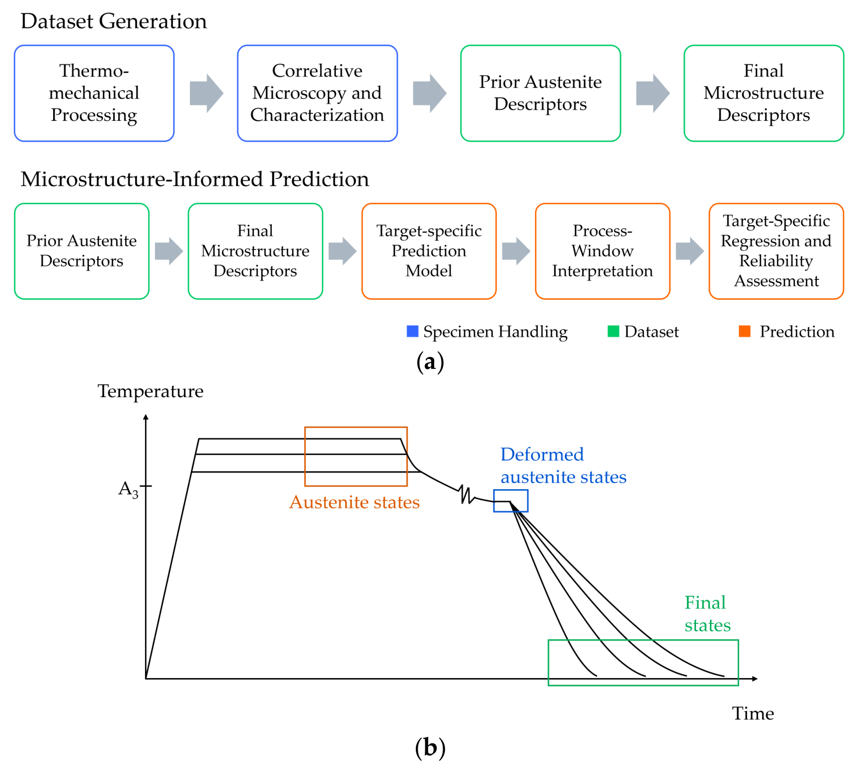
Figure 1 summarizes the structure of the study. The process–microstructure model workflow (Figure 1a) couples specimen-level dataset generation with target-specific prediction and process-window interpretation. The underlying experimental matrix (Figure 1b, parameter levels in Table 1) was designed to vary the austenitization temperature, deformation, and cooling rate independently, so that a broad range of prior austenite states and transformation regimes could be sampled within a single thermomechanical cycle. The resulting specimens were quantified by correlative microscopy and subsequently used to evaluate the microstructure-informed prediction models.

2.2. Correlative Microscopy Workflow

Correlative microscopy was used to obtain quantitative and physically meaningful descriptors of both the prior austenite state and the final room-temperature microstructure. The approach follows the general workflow established in previous works by Müller et al. [21] and Bachmann et al. [23,38], in which complementary microscopy techniques were combined on the same ROI through image registration. In the present study, LOM (LEXT Laser Scanning Microscope OLS 4100 (Olympus K.K., Tokyo, Japan)), SEM (Zeiss Merlin (Carl Zeiss AG, Oberkochen, Germany)), and EBSD (EDAX system (AMETEK Inc., Berwyn, PA, USA)) were used because they provide complementary information for steel microstructure analysis. LOM offers a rapid overview of the etched microstructure and provides suitable contrast for phase and morphology assessment over statistically relevant areas. SEM gives access to finer microstructural details that are not resolved sufficiently by LOM, such as bainitic or martensitic substructures. EBSD provides crystallographic information, grain boundary information, local misorientation, and image quality contrast, which are particularly useful for identifying boundaries, supporting prior austenite reconstruction, and improving the reliability of phase assignment [21].
For each specimen, the ROI was imaged by LOM (pixel size 0.127 µm; 4000 × 4000 pixels; 500 × 500 µm2 analyzed area), SEM (350× magnification), and EBSD (0.3 µm step size; 300 × 300 µm2 mapped area). This central region corresponds to the thermomechanically processed zone and is therefore the relevant area for evaluating the imposed heating, deformation, and cooling history. The resulting images were registered with the EBSD image quality map using Fiji/ImageJ (Version 1.53c) [39], following the procedure described in previous work [38]. The registered image stack enabled direct comparison of optical contrast, electron microscopy contrast, and crystallographic information at the same microstructural location. This correlative overlay was used to support ground-truth assignment for phase segmentation and morphology quantification, thereby reducing the dependence on a single contrast mechanism. While the image registration and correlative segmentation methodology was adopted from prior work [21,23,38], the new contribution of the present study is its application to the construction of an experimentally quantified process–austenite–final microstructure dataset for C-Mn and C-Mn-Nb steels. The derived descriptors were subsequently used for the statistical analysis and microstructure-informed model evaluation.

2.3. Definition of Transformation Products and Microstructural Targets

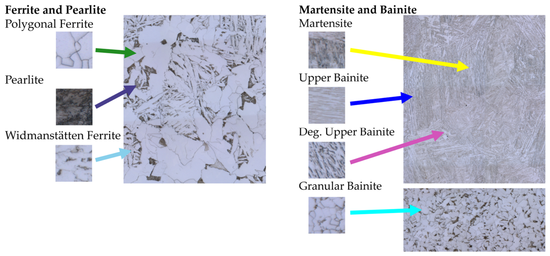
The final room-temperature microstructures were classified into seven transformation products covering ferritic–pearlitic, bainitic, and martensitic regimes. For the ferritic–pearlitic microstructures, polygonal ferrite (F) was treated as the primary matrix phase, while pearlite (P) was quantified as the carbon-enriched second phase. In specimens where the deformation and cooling conditions promoted non-equiaxed ferritic growth, Widmanstätten ferrite (WF) was considered as an additional ferritic transformation product, characterized by its plate-like structure. For the more complex bainitic–martensitic microstructures, needle-shaped martensite (M); upper bainite (UB) with ordered, parallel laths; degenerated upper bainite (DUB), which displayed a more disordered structure; and granular bainite (GB), consisting of a bainitic matrix and a carbon-rich second phase, were distinguished. The bainitic classification follows the terminology of Zajac et al. [33], allowing the model targets to reflect the microstructural differences that are often not resolved in conventional transformation modeling.
The separation of UB, DUB, and GB was retained as a deliberate methodological choice. Resolving the bainitic regime into three subclasses increased the descriptor–target complexity, but it also provided the regression models with finer-grained transformation-product information, allowing them to capture the differences among the bainitic subclasses from the prior austenite descriptors and cooling rate where the underlying separability permitted. DUB was treated as a separate target because it exhibits features intermediate between upper bainite and granular bainite, including a predominantly lath-like morphology with martensite/austenite constituents along the lath boundaries. This distinction was retained to avoid forcing visually and morphologically ambiguous regions into either UB or GB during ground-truth assignment. At the same time, the overlap between these bainitic subclasses was considered during model evaluation, because limited separability of individual bainitic targets may indicate either an insufficient sampling density, gradual microstructural transitions, or intrinsic ambiguity in the class definitions. Whether the present dataset supports the resolved subclass structure or whether the bainitic regime is better represented at a coarser level was therefore tested explicitly through the bainite target consolidation analysis in Section 3.3 (results in Section 5.3). The classification thus serves as both a metallurgical target definition and a stress test for data-driven separability.
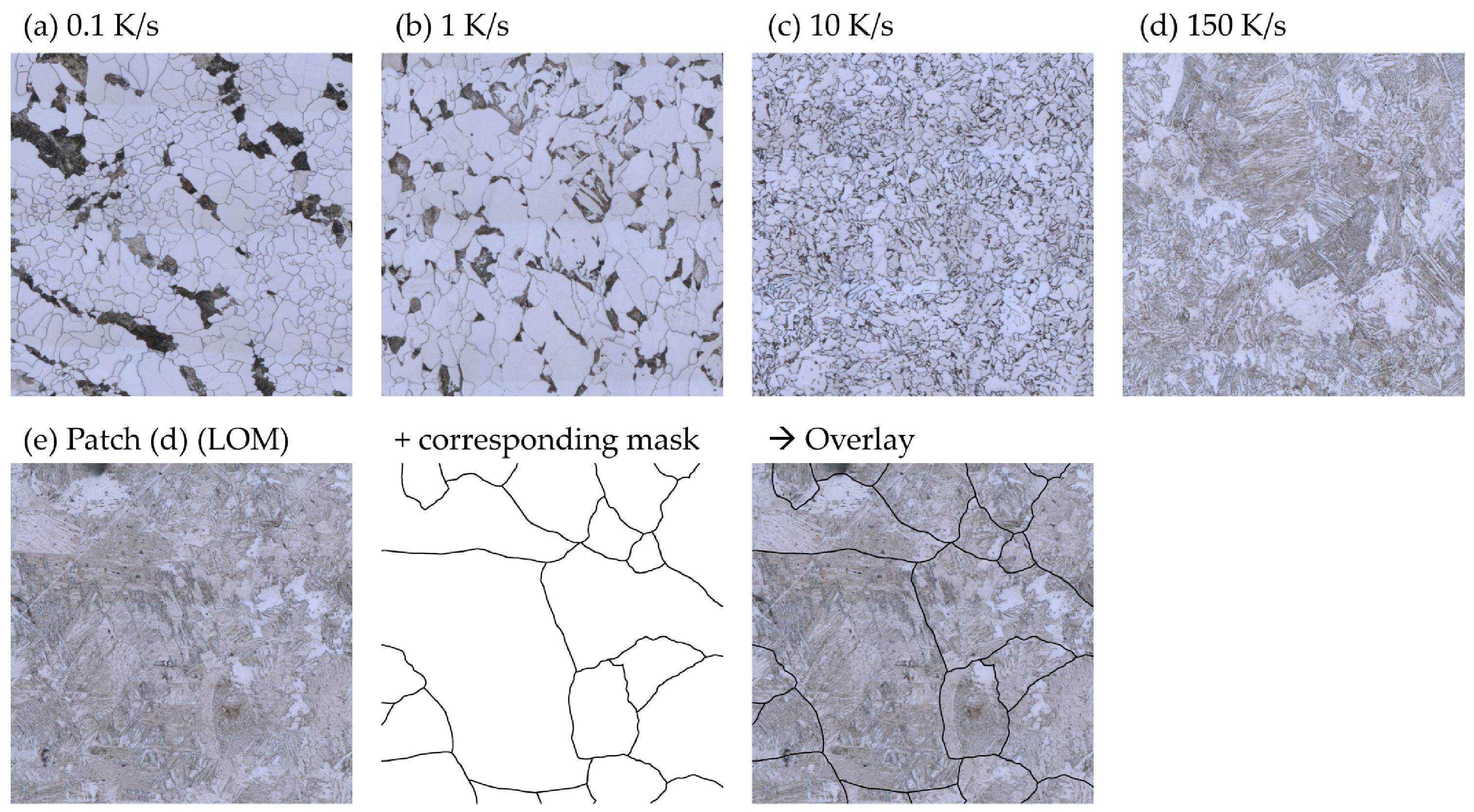
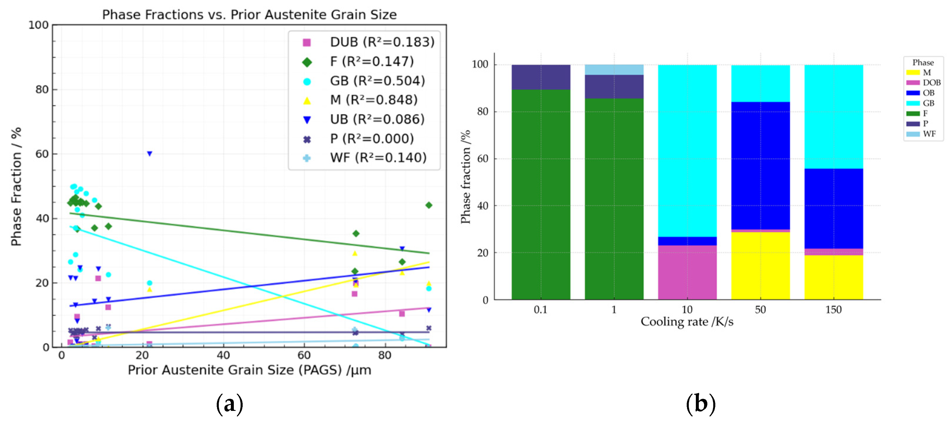
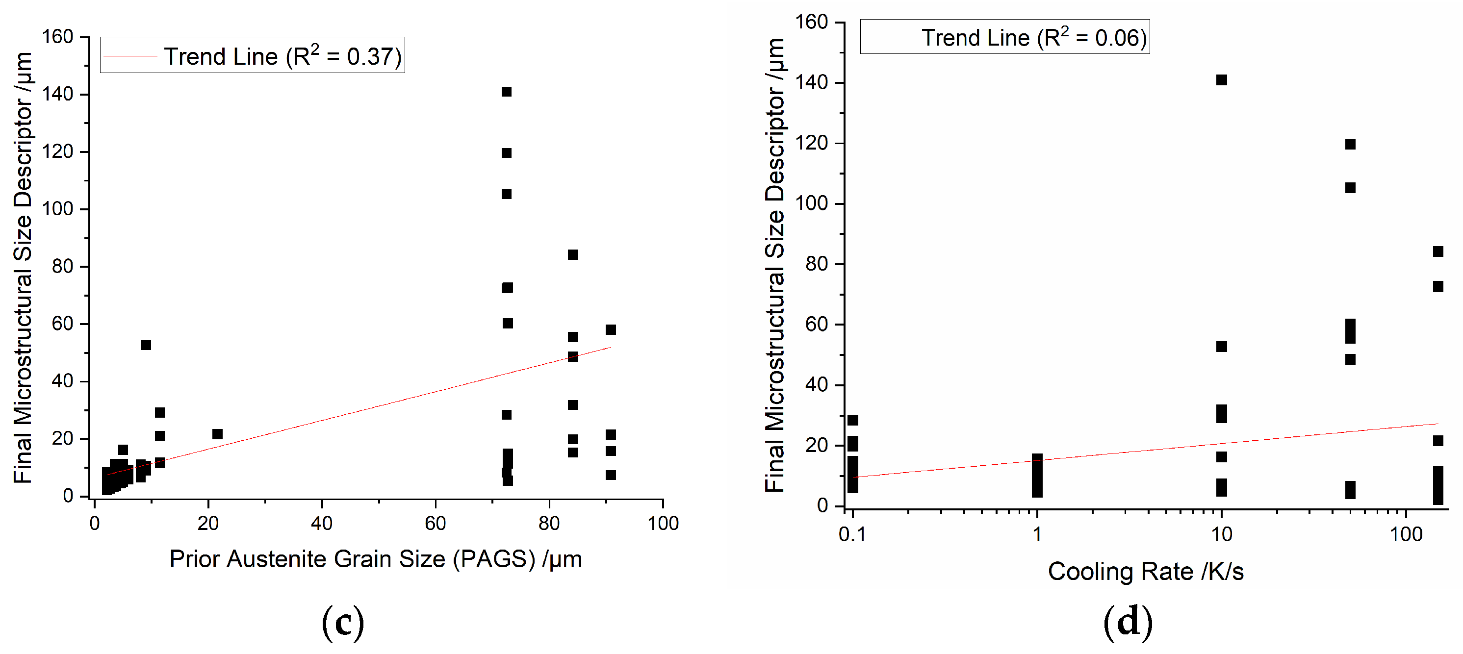
Figure 2 shows representative examples of the seven transformation products used as target classes for phase segmentation and phase fraction prediction. Figure 3 illustrates how these regimes arise from different cooling conditions and highlights the origin of target variability, including the high-cooling-rate cases, where mixed bainitic–martensitic morphologies contribute to increased scatter in the final size descriptor.

2.4. Phase Segmentation and Morphology Quantification

Phase segmentation and morphology quantification were performed using established image analysis workflows combined with the specimen-specific correlative microscopy data generated in this study. The ferritic–pearlitic and bainitic–martensitic microstructures were treated separately because their contrast mechanisms, characteristic length scales, and classification challenges differ substantially. The objective was to derive reproducible phase fraction and morphology descriptors for subsequent statistical analysis and model evaluation.
The ferritic–pearlitic microstructures were quantified using the pixel-wise segmentation workflow previously developed for dual-phase steel microstructures [23,40]. Pearlite was segmented as the carbon-enriched second phase within the ferritic matrix, while Widmanstätten ferrite was segmented manually because of its limited occurrence. Registered LOM, SEM, and EBSD overlays were used to support correction of phase and grain boundary masks where optical contrast alone was insufficient.
The bainitic–martensitic microstructures were quantified using the patch-based classification workflow of Bachmann et al. [23,38]. Registered image stacks containing EBSD image quality data, EBSD grain boundary information, LOM images, and SEM images were used to extract 64 × 64 pixel patches, corresponding to 9.4 µm × 9.4 µm. The training dataset contained 3032 patches for martensite, 3053 for upper bainite, 2793 for degenerated upper bainite, and 5797 for granular bainite. A convolutional neural network (CNN) with an XCeption backbone was trained for these four classes and applied to complete the LOM micrographs using a sliding-window approach [38,41].
A classification confidence threshold of 90% was applied to the bainitic–martensitic segmentation. Regions below this threshold were assigned to an “unknown” class and were not forced into one of the target classes. No manual correction was performed after this automated segmentation step. On the validation dataset, the classifier achieved an overall accuracy of 0.79, and class-wise accuracies of 0.68 for DUB, 0.90 for GB, 0.82 for M, and 0.72 for UB.
The morphology descriptors were calculated from the binary grain boundary or phase boundary masks using scikit-image [42]. For the ferritic–pearlitic microstructures, the size descriptor refers primarily to the ferrite grain size. For the bainitic–martensitic microstructures, the corresponding size descriptors represent boundary-delimited units, such as packets, islands, blocks, or lath aggregates. The initial set of 20 size-, shape-, orientation-, and connectivity-related morphology descriptors (Appendix A, Table A1) contained largely redundant geometric quantities. For example, the equivalent diameter, area, and perimeter carry closely related size information. To avoid strongly collinear variables while preserving physically interpretable descriptors, redundancy clusters were identified from pair-wise correlations between descriptors (R2 ≥ 0.7), and one representative per cluster was retained. Within each cluster, the representative was selected based on physical interpretability and numerical stability across microstructure regimes, supported by MRMR [43] and F-test ranking (see Appendix A). For comparability between the prior austenite state and final microstructure, the same representatives, equivalent diameter and axial ratio, were used both as the input descriptors (PAGS, prior austenite axial ratio) and final morphology targets. The segmentation and quantification routes are summarized in Table 2.

2.5. Descriptor Definition and Feature Selection

The quantified processing and microstructure information was converted into a tabular dataset, in which each specimen was represented by physically interpretable input descriptors and prediction targets. The input descriptors were the PAGS, prior austenite axial ratio, dislocation density, and cooling rate. The PAGS and axial ratio were obtained from the reconstructed or boundary-segmented prior austenite structure. Austenite reconstruction from the EBSD raw data was performed in MATLAB (Version R2025a) using an MTEX-based implementation [44,45]. The full reconstruction pipeline, including the assumed orientation relationship and the parent-grain identification scheme, is proprietary and cannot be disclosed. The reconstructed prior austenite maps were verified against the etched microstructure and EBSD image quality contrast on the same ROI before the PAGS and axial ratio were derived from the resulting boundary masks.
The dislocation density was estimated from the deformation response recorded during thermomechanical simulation using the Taylor relation [14], following Bengochea et al. [6]. The friction-corrected flow stress was used as the stress input, while the shear modulus and Burgers vector were calculated as temperature-dependent quantities according to Laub [46] and Seki and Nagata [47]. The resulting value was treated as an effective descriptor of the deformation-induced defect state of the austenite, rather than as a direct microscopic dislocation-density measurement.
The prediction targets describe the final room-temperature microstructure and selected mechanical response. They comprise the phase fractions, morphology descriptors, pearlite mean free path length (MFPL), and Vickers hardness HV0.1. The complete input target structure is summarized in Table 3.
All model evaluations were therefore based on physically interpretable descriptors rather than abstract image features. This was to support metallurgical interpretation of the model results and to enable a comparison between the model-derived feature rankings and established transformation behavior.

2.6. Dataset Disclosure Under Confidentiality Constraints

The raw dataset, source code, and detailed steel chemistries—including the exact compositions of the investigated C-Mn and C-Mn-Nb steels—cannot be made publicly available because they are part of ongoing industrial research and are subject to contractual third-party confidentiality restrictions. To support critical assessment despite these restrictions, the present manuscript follows a closed-data transparency strategy. The information that can be disclosed within these bounds includes the experimental design matrix (Table 1); variable and target definitions (Table 3); the segmentation and quantification routes used to derive each descriptor (Table 2); the preprocessing and feature-selection steps (Section 2.5 and Appendix A); the dataset structure across steel variants, cooling-rate groups, and transformation-regime subsets (Table 4); the validation protocol and model selection criteria (Section 3.2); representative micrographs (Figure 2 and Figure 3); and full target-specific performance metrics for each candidate model family (Section 5 and Tables 7 and 8). The results are correspondingly interpreted within this disclosed processing and microstructure domain and are not used to derive composition-resolved alloy design rules.

2.7. Dataset Structure and Target Complexity

Table 4 reports the number of specimens available for the full dataset, steel variants, cooling-rate groups, and transformation-regime subsets used for model evaluation. This overview defines the sampled processing domain and helps distinguish well-represented regimes from sparsely sampled transformation conditions. The target-specific complexity is reported alongside the model performance metrics in Section 5 (Table 7), where it is used to interpret whether limited prediction accuracy reflects model limitations or sparse target sampling.

3. Data-Driven Modeling and Validation Strategy

3.1. Prediction Tasks and Model Hierarchy

The modeling step was designed to evaluate whether the experimentally quantified prior austenite descriptors, combined with the cooling rate, could predict the final microstructure and hardness within the investigated processing domain. All targets listed in Table 3 were considered within a common modeling framework; however, they were not expected to be equally predictable because they differed in their occurrence frequency, transformation range, target variance, and segmentation uncertainty. Therefore, the targets were grouped into reliability levels before model evaluation to guide interpretation of the results.
The a priori quantitative targets were expected to comprise the ferrite fraction, pearlite fraction, final size descriptor, pearlite MFPL, and Vickers hardness HV0.1, all of which occurred over comparatively broad or continuous ranges and were the main basis for assessing the process-window prediction capability. The semi-quantitative targets were expected to comprise the granular bainite, upper bainite, and degenerated upper bainite phase fractions and the final axial ratio—physically relevant outputs affected by narrower transformation windows, class overlap, lower phase fractions, or boundary-definition sensitivity. The Martensite and Widmanstätten ferrite were expected to be diagnostic-only because of their limited occurrence and expected low data-driven separability. Their prediction performance was used to identify the limits of the framework and to indicate where additional targeted experiments are required.

3.2. Model Families, Baseline Comparison, Evaluation Metrics, Reliability Classes

A set of regression models was evaluated to cover linear, kernel-based, tree-based, and gradient-boosting approaches without restricting the analysis to a single algorithmic assumption. The implementation was based on scikit-learn-compatible regression workflows [48], including support vector regression [49], Random Forest [50], ExtraTrees [51], XGBoost [52], histogram-based gradient boosting [53], CatBoost [54], and LightGBM [55]. These model families cover a range of model complexities and are commonly used for tabular regression problems in materials informatics and microstructure–property modeling [56]. A dummy regressor was included as a baseline to verify whether each model provided meaningful predictive value beyond simply predicting the central tendency of the training data.
All models were implemented in a common preprocessing and validation framework. The dataset was split into training and test subsets, with 25% of the specimens held out for testing, balancing test set statistical adequacy with training set richness. The test set was drawn by random sampling. To assess the sensitivity of the results to the data partition, the complete workflow, comprising the training–test split, 5-fold cross-validation on the training subset, and target-specific model selection, was repeated for six different random splits. For each split, it was verified that all transformation regimes and both alloy variants were represented in the held-out test set. R2 and RMSE are reported together with their standard deviation over the six runs. Because model selection was repeated within each run, the best-performing model for a given target could differ between runs. Model selection was performed on the training data using 5-fold cross-validation. Standardization was applied for scale-sensitive models, such as support vector regression, while tree-based and boosting models were evaluated without relying on feature scaling. Because the prediction targets differed in their variance, occurrence frequency, and physical meaning, model selection was performed separately for each target using cross-validated performance metrics. The best-performing target-specific models were then combined into a common multi-output prediction workflow for subsequent evaluation and interpretation. The model families and selection criteria for the regression workflow are summarized in Table 5.
Model performance was evaluated using complementary metrics to account for both predictive accuracy and target-specific difficulty. For each target, the coefficient of determination (R2) and root mean square error (RMSE) were reported and used to interpret whether poor performance resulted primarily from model limitations or from sparse and imbalanced target distributions.
The following reliability classes were assigned using the combined evidence from the model metrics, baseline improvement, target distribution, and physical interpretability.
  • Quantitative: High R2, low normalized RMSE, and clear improvement over the baseline. These targets are considered usable for process-window interpretation within the investigated domain.
  • Semi-quantitative: Moderate model performance combined with physically meaningful trends. These targets are interpreted as trend indicators rather than precise quantitative predictions.
  • Diagnostic only: Low or negative R2, limited baseline improvement, sparse occurrence, or strong target imbalance. These targets are not considered quantitatively predictable with the present dataset but are retained to identify the limits of the framework and guide future targeted experiments.

3.3. Controlled Synthetic Data and Target Consolidation

Controlled synthetic data generation was evaluated as an interpolation-based self-consistency analysis, rather than as a substitute for additional experiments [57,58,59]. In fact, it added no independent experimentation and was further not suited as a form of model validation. Synthetic input candidates were generated by uniform random sampling within the experimentally observed bounds of the continuous descriptors (PAGS, prior austenite axial ratio, and dislocation density). Because the cooling rate was experimentally varied across five discrete levels (0.1, 1, 10, 50 and 150 K/s), the candidate cooling rates were drawn from these levels with a small multiplicative log-uniform jitter of ±15% and clipped to the experimental range. This preserved the experimental cooling-rate structure as a regime rather than a continuous variable while avoiding dense synthetic clusters at the discrete levels. As a consequence, augmentation densified the input space near the experimental cooling rates rather than bridging the gaps between them.
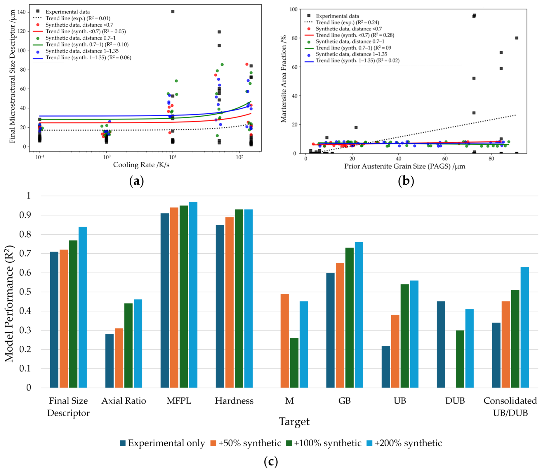
The candidates were standardized using a scaler fit on the training data and filtered in the standardized four-dimensional input space using a one-nearest-neighbor proximity criterion. A maximum standardized distance of 1.35 to the nearest training point was used as the rejection threshold, chosen as a balance between local consistency with the experimental data and sufficient acceptance rate. The specific value was selected by stratifying the synthetic candidates into three distance bands (≤0.7, 0.7–1.0, and 1.0–1.35; Figure 7a,b) and confirming that the candidates in all three bands fell within the value ranges and trend behavior of the experimental data, while admitting a sufficient acceptance rate for the requested augmentation sizes. The predicted target values for the accepted candidates were obtained from the trained per-target models, and the phase fraction predictions were renormalized to sum to 100% to preserve physical plausibility. Generation continued until the requested number of unique accepted candidates was reached, corresponding to 50%, 100%, or 200% of the experimental dataset size. Because the synthetic target values were generated by the trained per-target models themselves, the augmentation acted as a pseudo-labeling or self-consistency regularization rather than as injection of independent information. The performance metrics obtained after augmentation therefore do not constitute independent validation; they partly reflect how well the retrained models reproduced the predictions of the generating models in the augmented region. The effect of augmentation was evaluated target-wise, and all statements regarding predictive performance are based on the experimental-only metrics reported in Table 7.
As a second robustness test, the bainitic subclasses of upper bainite and degenerated upper bainite were combined into a consolidated target and compared with their separate predictions. The consolidation was not intended to redefine the metallurgical classification but to test whether the broader bainitic regime could be predicted more robustly than the individual subclasses, given their partially overlapping formation conditions and gradual morphological transitions.

3.4. Feature Importance and Physical Consistency

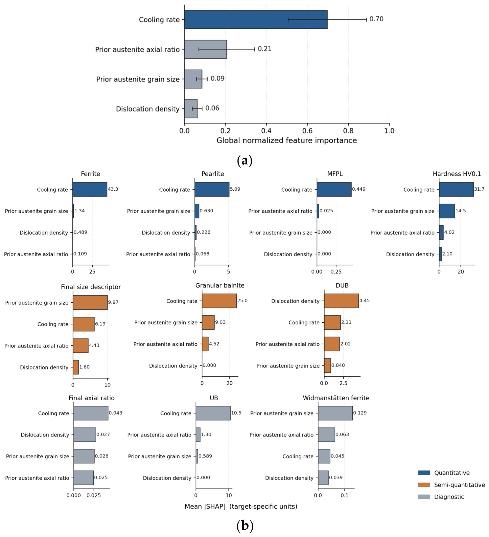
A feature importance analysis was used to assess whether the trained models relied on physically meaningful descriptors. For the best-performing target-specific models, feature rankings were determined using SHAP values [56]. The analysis was performed separately for each prediction target to identify the dominant descriptors controlling the individual phase fractions, morphology descriptors, and hardness. Particular attention was given to whether the identified rankings were consistent with established metallurgical expectations, such as the dominant influence of cooling rate on ferrite and pearlite formation, the relevance of PAGS for displacive transformation products and final size descriptor, and the expected connection between phase constitution and hardness.
The feature importance was interpreted primarily on a target-wise basis. Raw SHAP magnitudes depend on the scale, variance, and units of the respective target variable and should therefore not be compared directly across different outputs unless normalized. The purpose of the analysis was to evaluate whether each model learned physically plausible process–microstructure relationships within the investigated domain.

4. Baseline Physical Trends and Sanity Checks

Before evaluating the data-driven models, the dataset was analyzed for physically expected process–microstructure relationships. This step served as a plausibility check for the experimentally derived descriptors and provided a baseline for interpreting the subsequent model results. Linear or monotonic trend analyses were used only as descriptive indicators of dominant relationships, not as predictive models for the full transformation behavior.

4.1. Process Parameters and Prior Austenite State

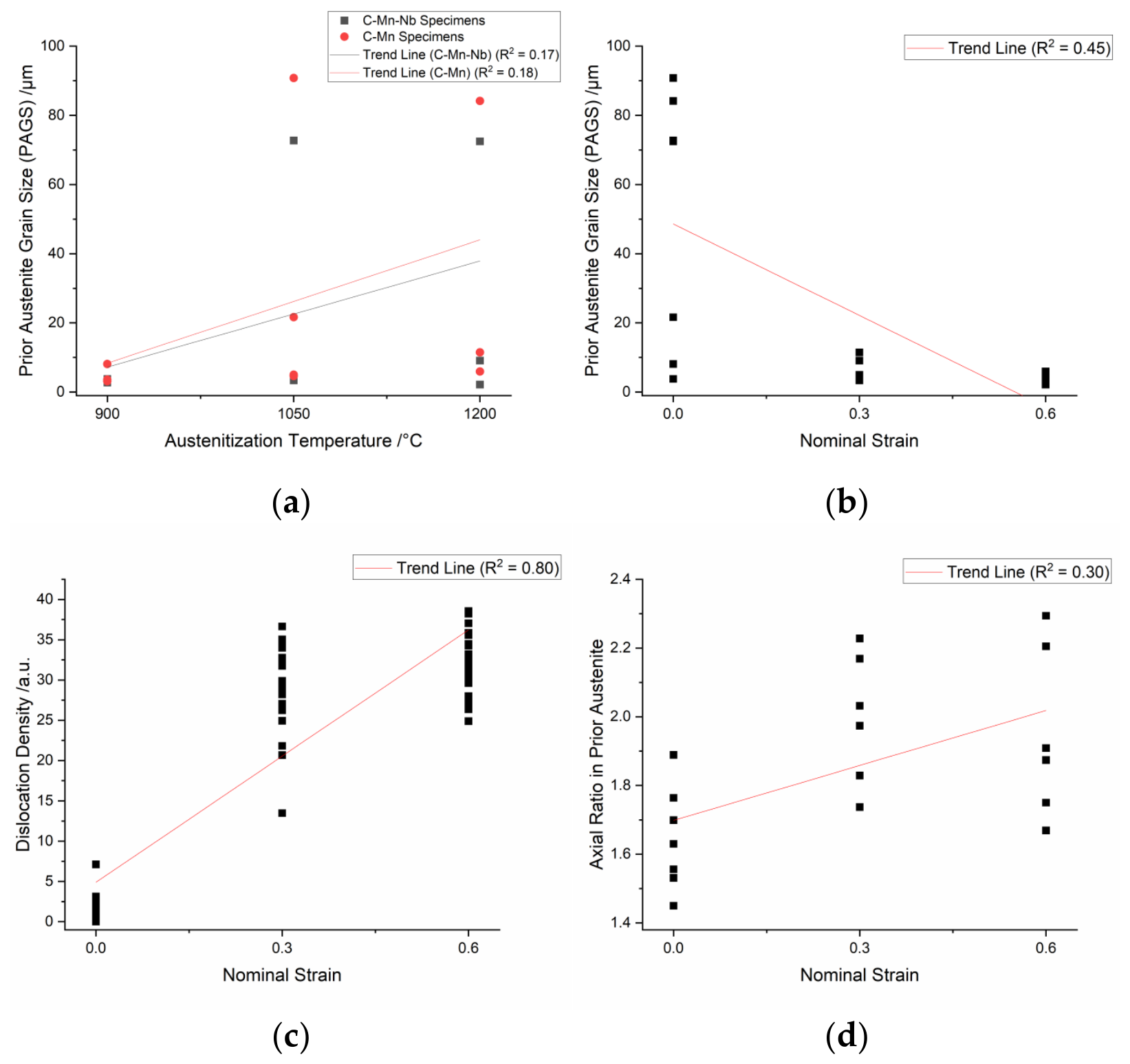
The first consistency check addressed the relationship between the thermomechanical processing parameters and the quantified prior austenite descriptors. Figure 4 summarizes the effect of austenitization temperature, nominal strain, and steel variant on the PAGS, axial ratio, and dislocation density. The observed trends are consistent with established transformation and recrystallization behaviors. That is, increasing deformation reduced the PAGS and increased the axial ratio, while a higher austenitization temperature promoted grain growth. The estimated dislocation density increased primarily with deformation, as expected from its derivation from the friction-corrected flow stress. The Nb-containing variant showed a measurable but weaker effect on the PAGS compared with the deformation and austenitization temperature. The Nb-related trend is interpreted only within the investigated material pair and is not used to derive composition-resolved alloy design rules.
The relative influence of the processing parameters was assessed using standardized regression coefficients as well as F-test ranking (Table 6). Deformation was identified as the dominant factor for the PAGS and axial ratio, while the austenitization temperature showed the expected secondary contribution to grain growth. For the dislocation density, deformation was the dominant predictor. These results support the physical plausibility of the input descriptors used for subsequent model evaluation, but were not used for model input selection.

4.2. Prior Austenite Descriptors, Cooling Rate, and Transformation Products

The second consistency check addressed the relationship between the prior austenite descriptors, cooling rate, and final room-temperature microstructure. Figure 5 shows the main transformation trends using individual data points. The cooling rate was the dominant descriptor separating the ferritic–pearlitic, bainitic, and martensitic transformation regimes. Ferrite and pearlite occurred primarily at lower cooling rates, whereas bainitic and martensitic constituents were associated with higher cooling rates and narrower transformation windows [1,2]. This distribution already indicates why ferrite and pearlite are more suitable for quantitative regression than rare or narrowly occurring targets such as Widmanstätten ferrite, martensite, and individual bainitic subclasses.
The PAGS also affected the final microstructure. Larger prior austenite grains tended to be associated with a larger final size descriptor and, depending on the cooling conditions, with increased occurrence of displacive transformation products [35,60,61]. However, the scatter was substantial because the final morphology was governed by the combined influence of prior austenite state, cooling rate, and transformation product. The relationship between the final size descriptor and cooling rate was therefore interpreted with caution, especially at high cooling rates, where the descriptor may have represented bainitic packets, martensitic blocks, islands, or lath aggregates rather than ferrite-equivalent grains.
Hardness followed the expected dependence on phase constitution. Because the dataset is bimodal—specimens are either fully ferritic–pearlitic or fully martensitic–bainitic—the hardness response separated into two well-defined groups: 137 ± 13 HV0.1 for ferritic–pearlitic microstructures and 204 ± 52 HV0.1 for martensitic–bainitic microstructures, consistent with the higher dislocation density and finer microstructural units in the displacive products [62]. These baseline trends confirm that the dataset captures physically meaningful process–microstructure–property relationships. At the same time, the observed scatter illustrates why nonlinear, target-specific models are required for subsequent prediction.

5. Microstructure-Informed Prediction Performance

The prediction performance of the microstructure-informed models was evaluated for all targets defined in Table 3 using the full experimental dataset. The results are interpreted according to the reliability hierarchy introduced in Section 3.1, because the targets differed substantially in their occurrence frequency, transformation range, intrinsic variance, and segmentation uncertainty. The aim of this section is therefore not to identify a single globally best model, but to determine which final microstructure and property targets can be predicted quantitatively, which can be interpreted as trends, and which mainly reveal the current limits of the dataset.

5.1. Model Performance and Target Reliability

Table 7 summarizes the target-specific prediction performance for the full dataset. For each target, the best-performing model was selected based on the cross-validation procedure and evaluated using the reliability criteria defined in Section 3.2 (i.e., R2 and RMSE). Table 7 lists the best model per target together with its R2 and RMSE. In addition, both the mean and error (standard deviation) over the six repeated runs are given to indicate the sensitivity of the results to the data partition. Because model selection was repeated in each run, the mean and error also cover runs in which a different model was selected as the best for a given target. It therefore describes the stability of the target-specific prediction workflow as a whole rather than the variability in a single fixed model. Because the targets differed in their variance and occurrence frequency, the model results are interpreted together with the intrinsic target complexity reported in Table 4.
The quantitative targets showed the most reliable performance. The ferrite and pearlite fractions were predicted with high accuracy, consistent with their broad occurrence over the investigated cooling-rate range and their strong dependence on the transformation regime. The pearlite MFPL and Vickers hardness HV0.1 also showed useful predictive capabilities within the investigated domain. The final size descriptor is regarded as semi-quantitative on the basis of its lower R2, but nonetheless retains useful predictive capability for screening purposes (Table 7). The results indicate that the combination of prior austenite descriptors and cooling rate can support process-window screening for dominant, well-sampled transformation products and selected morphology/property indicators.
For granular bainite, the performance was moderate and stable across runs (R2 = 0.61 ± 0.03) and is interpreted as a semi-quantitative trend target. For upper bainite, the performance remained low in all runs (R2 = 0.24 ± 0.07). The degenerated upper bainite reached R2 = 0.45 for the best model, but the mean over six runs was only 0.02 ± 0.27. The favorable single-run result therefore depended strongly on the data partition, and both subclasses are treated as diagnostic targets. For martensite and Widmanstätten ferrite, none of the candidate models outperformed the baseline reliably, and they are like-wise treated as diagnostic. The low or negative R2 values for these outputs—where a negative R2 means the model performs worse than when predicting the training data mean—reflect the insufficient sampling density of the present experimental matrix in the corresponding transformation windows rather than physically meaningless transformation behavior or algorithmic failure.

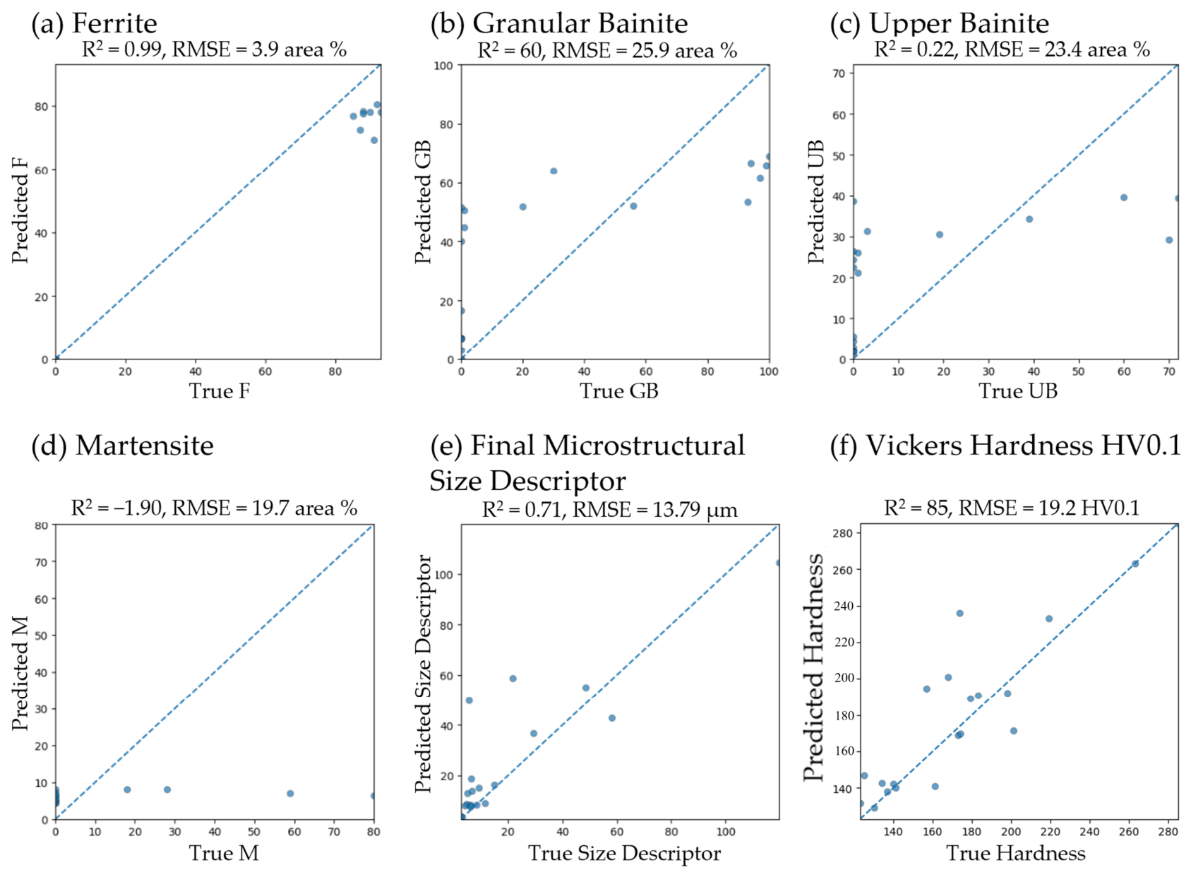
5.2. Representative Parity Plots and Transformation-Regime Dependence

Representative parity plots are shown in Figure 6 for selected quantitative, semi-quantitative, and diagnostic targets. Ferrite, pearlite, hardness, and the final size descriptor show predictions closer to the ideal parity line, reflecting their broader occurrence and stronger relation to the dominant input descriptors. In contrast, martensite and individual bainitic subclasses show larger scatter, consistent with their narrower transformation windows and stronger sensitivity to local microstructural classification.
The model is most reliable for targets associated with well-sampled ferritic–pearlitic transformations and selected continuous descriptors such as hardness. The predictions become less robust in regimes where bainitic and martensitic products overlap or where the physical meaning of morphology descriptors changes from ferrite grains to boundary-delimited packets, islands, blocks, or lath aggregates. The parity plots therefore support the reliability classification in Table 7 and show that the framework is most suitable for process-window screening of dominant, well-represented microstructure features.

5.3. Effect of Controlled Augmentation and Bainite Target Consolidation

Controlled synthetic data generation was evaluated as a self-consistency check. Synthetic input candidates were generated only within the measured input range and filtered using a one-nearest-neighbor proximity criterion in standardized feature space, so that the retained samples represented interpolation points within the experimental domain rather than extrapolated processing conditions (Figure 7). Because the synthetic target values were produced by the same trained per-target models that were subsequently retrained on the augmented dataset, the procedure tested whether the models remain internally consistent under interpolation, not whether they generalize better to independent data. The assessment of predictive performance therefore relied exclusively on the experimental-only metrics in Table 7, and changes in R2 after augmentation should not be read as improved predictive accuracy. The augmentation results in Table 8 are reported as a limitation-aware stability analysis rather than as independent validation.
The effect of augmentation was evaluated by comparing models trained on the experimental dataset alone with models trained using additional synthetic data corresponding to 50%, 100%, and 200% of the original dataset size (Table 8).
For well-sampled targets, such as ferrite, pearlite, MFPL, final size descriptor, and hardness, R2 remained stable or increased with an increasing synthetic fraction. This behavior was expected by design—in fact, the synthetic labels follow the smooth response surface of the generating models, so a larger synthetic fraction makes the augmented dataset easier to fit. The increase therefore shows that the models remain internally consistent under interpolation within the experimental domain. For sparse or threshold-controlled targets, such as martensite, Widmanstätten ferrite, and weakly separated bainitic subclasses, R2 changed non-monotonically. The proximity criterion preferentially retained synthetic samples in well-populated regions of the descriptor space, close to the dataset mean, while the narrow transformation windows in which these products occur remained undersampled. Thus, the apparent R2 shifted with each resampling of the synthetic distribution rather than converging. Even where R2 increased for these targets (e.g., for martensite, from −1.90 to 0.45), this reflects the changed sample geometry and the self-consistency of the pseudo-labels rather than an improved representation of the underlying transformation boundary.
Bainite target consolidation was evaluated as a second robustness test. Although upper bainite and degenerated upper bainite are metallurgically distinguishable, their formation conditions overlap and their morphologies change gradually, which limits how well they can be separated in a data-driven manner. The repeated runs in Table 7 support this, as the degenerated upper bainite showed the strongest partition dependence of all bainitic targets (R2 = 0.02 ± 0.27). Both subclasses were therefore combined into a single target to test whether the broader bainitic regime could be predicted more robustly than its individual subclasses. This consolidation serves only as a model evaluation strategy and is by no means proposed as a new metallurgical classification. Based on the experimental data alone, the consolidated target reached R2 = 0.34 (Table 8), a moderate gain over upper bainite and the six-run mean performance for upper bainite. This suggests that the present dataset may capture the broader bainitic regime more reliably than the distinction between its subclasses. The further increase in R2 after augmentation is subject to the self-consistency limitation described above and is not interpreted as improved predictability.
Overall, controlled augmentation and target consolidation are interpreted as limitation-aware robustness analyses. Augmentation demonstrates that the models remain internally consistent under interpolation for well-represented targets, but it provides no independent evidence of improved predictive performance. Neither approach can replace targeted experiments in sparsely sampled transformation regimes. In particular, additional experiments in the high-cooling-rate and mixed bainitic–martensitic regimes remain necessary to improve the quantitative prediction of martensite and individual bainitic subclasses.
Together with the repeated experimental runs (Table 7), these findings confirm that the current framework is most reliable when the target is well represented in the experimental dataset and physically less ambiguous. The following section therefore summarizes the practical implications for process-window interpretation and identifies the transformation regimes where additional targeted data are required.

5.4. Feature Importance and Physical Consistency

A feature importance analysis was used to evaluate the physical consistency of the trained models. SHAP values were calculated for the best-performing target-specific models and interpreted primarily within each target, because raw SHAP magnitudes depend on the target scale, variance, model type, and output units. Global rankings were calculated only for reliable and semi-reliable targets to avoid distortion by diagnostic outputs.
The cooling rate and PAGS emerged as the dominant descriptors across reliable targets, consistent with their expected influence on the transformation regime, nucleation density, and final morphology. Ferrite and pearlite were mainly controlled by the cooling rate, while the final size descriptor was linked to the PAGS and austenite morphology. Hardness was governed indirectly through the descriptors controlling phase constitution. The bainitic subclasses showed less stable rankings, reflecting class overlap and reduced data-driven separability. Martensite showed physically plausible sensitivity to the cooling rate and PAGS, but because of its weak prediction reliability, its feature ranking was interpreted only diagnostically. Figure 8 summarizes the normalized global feature rankings for reliable and semi-reliable targets together with selected target-specific SHAP rankings.
These results support the physical consistency of the models for well-represented targets while remaining consistent with the metallurgical expectations that sparse or overlapping transformation products require additional targeted experiments before quantitative process-window prediction is possible.

5.5. Interpretation of Weak and Diagnostic Targets

The weakest model performance was obtained for the targets that combine metallurgical complexity with limited statistical representation. Martensite is associated with threshold-like transformation behavior and occurs primarily in the high-cooling-rate regime [9,60]. Consequently, the number of informative nonzero observations is limited. Widmanstätten ferrite is also difficult to predict because it occurs only under specific conditions [36,63] and is represented by a small number of samples. For upper bainite and degenerated upper bainite, the main limitation is not only the number of data points, but also the gradual morphological transition and partial overlap between the classes, which is reflected in the high run-to-run variability for DUB (Table 7). This reduces data-driven separability even when the phases are metallurgically distinguishable.
These results do not imply that the corresponding transformation products are physically uncontrolled. Instead, they show that the current experimental matrix is insufficiently dense in the relevant transformation windows for quantitative regression of these targets. Therefore, martensite, Widmanstätten ferrite, and weakly separated bainitic subclasses are excluded from the quantitative process-window recommendations in the present study and are used instead to identify where targeted additional experiments would be most valuable.
By contrast, ferrite, pearlite, MFPL, final size descriptor, and hardness provide the most useful process-window information. The current framework is therefore best suited for screening dominant transformation regimes and selected morphology/property indicators within the investigated processing domain, while rare or overlapping transformation products require further targeted sampling before robust quantitative prediction can be expected.
Overall, the model provides useful process-window information for dominant, well-sampled transformation products and selected morphology/property indicators, but it should not be interpreted as a universal predictor for rare or narrowly occurring phases. This distinction defines the practical design relevance and current limitations of the framework, which are discussed in the following section.

6. Design Implications, Limitations, and Future Development

Within the investigated C-Mn/C-Mn-Nb processing domain, the framework supports microstructure-informed screening of dominant transformation products and selected morphology and property indicators. The ferrite and pearlite fractions, pearlite MFPL, final size descriptor, and hardness provide a reliable basis for process-window interpretation, enabling comparison of thermomechanical process routes, identification of physically meaningful descriptor trends, and prioritization of experiments within the studied parameter space. Narrowly occurring or weakly separated transformation products—martensite, Widmanstätten ferrite, and individual bainitic subclasses—are best interpreted as diagnostic indicators within the present C-Mn and C-Mn-Nb showcase. Their lower predictability reflects the specific occurrence frequencies and transformation windows of this experimental matrix rather than a general property of the descriptor-based approach, and they are retained in the framework as targeted starting points for further experimental sampling.
The framework is positioned as a complementary, experimentally grounded tool for process-window screening and interpretation rather than as a certification-grade transformation model. Its applicability covers the investigated processing and microstructure domain, and extension to other alloy systems, compositions, or process routes is a natural next step that requires additional validation. The dataset of 80 specimens establishes that experimentally quantified austenite descriptors can support physically consistent screening across the sampled processing domain, spanning ferritic–pearlitic, bainitic, and martensitic transformation regimes. It does not yet resolve the full variance of overlapping bainitic subclasses, threshold-driven displacive products, or the multivariate coupling between prior austenite state and cooling path—these remain open and will require further targeted experiments in the relevant transformation windows. Because the detailed steel chemistries, raw data, and code are subject to confidentiality restrictions, the closed-data transparency strategy used here defines the investigated domain through statistical summaries and full target-specific performance metrics rather than through open data release.
Correlative microscopy generates high-fidelity ground truth at substantial experimental cost, which makes it especially valuable as a targeted calibration source for downstream modeling rather than as a routine production measurement. The most productive next step will therefore be to combine focused correlative datasets with broader lower-cost process data and physically based constraints. Targeted experimental campaigns across the high-cooling-rate and mixed bainitic–martensitic regimes, supported by uncertainty-guided data acquisition and hybrid modeling using TTT/CCT diagrams or deterministic transformation models [8], would extend quantitative prediction to the diagnostic targets and expand the reliable prediction domain.

7. Conclusions

This work evaluated whether experimentally quantified prior austenite descriptors, obtained by correlative microscopy on a Gleeble-based thermomechanical matrix of C-Mn and C-Mn-Nb specimens, can support the physically consistent prediction of final transformation products and selected mechanical responses. By combining a fully disclosed experimental design matrix, target distributions, intrinsic variance, and target-specific model evaluation, the framework enables critical assessment of model reliability despite the closed underlying data.
Within the investigated processing domain, reliable predictions were obtained for the ferrite and pearlite fractions, pearlite mean free path length, final size descriptor, and Vickers hardness. These outputs support process-window screening, comparison of thermomechanical routes, and prioritization of further experiments. However, predictions for martensite, Widmanstätten ferrite, and individual bainitic subclasses remained limited by their sparse occurrence, narrow transformation windows, and gradual morphological transitions between classes. Controlled synthetic data generation showed that the models remained internally consistent under interpolation for well-sampled targets. Because the synthetic labels were generated by the models themselves, the resulting metric changes do not constitute independent validation. Neither augmentation nor bainite target consolidation resolved the limitations of the sparse targets, which can only be addressed by targeted experiments in undersampled transformation regimes.
Three main directions follow directly from these findings. First, targeted experimental campaigns in the high-cooling-rate and mixed bainitic–martensitic regimes would densify the transformation windows currently classified as diagnostic and convert at least some of them into quantitatively predictable outputs. Second, hybrid modeling strategies that combine experimentally quantified austenite descriptors with physically based constraints from TTT/CCT diagrams or deterministic transformation models offer a route to extend the framework beyond its current screening role without requiring full open-data reproducibility. Third, the closed-data transparency strategy demonstrated here—disclosure of the design matrix, target distributions, intrinsic variance, and full target-specific performance metrics—provides a template for evaluating data-driven materials models built on industrially restricted datasets, an increasingly common situation as industry–academia collaborations grow. Together, these directions position the framework as a basis for further development rather than as a finished predictive tool.

Author Contributions

Conceptualization: M.S., B.-I.B., M.M., M.W.-M., T.S. and F.M.; methodology: M.S. and B.-I.B.; software: M.S.; validation: M.S., B.-I.B., M.M., D.B., M.W.-M. and T.S.; formal analysis: M.S.; investigation: M.S.; resources: D.B., M.W.-M., T.S. and F.M.; data curation: M.S.; writing—original draft preparation: M.S.; writing—review and editing: M.S., B.-I.B., M.M., D.B., M.W.-M. and T.S.; visualization, M.S.; supervision, D.B., T.S. and F.M.; project administration, D.B., T.S. and F.M.; funding acquisition: D.B., M.W.-M., T.S. and F.M. All authors have read and agreed to the published version of the manuscript.

Funding

Open access funding was enabled and organized by Projekt DEAL.

Data Availability Statement

The datasets presented in this article are not readily available because they are part of ongoing industrial research and subject to restrictions by a third party (Aktien-Gesellschaft der Dillinger Hüttenwerke). Requests to access the datasets should be directed to the corresponding author.

Acknowledgments

The authors would like to acknowledge Maita Roberts-Zimmer, Eric Detemple, and Andreas Hoffmann for conducting the Gleeble experiments and Darius Weidner for assistance in image registration. During the preparation of this manuscript/study, the authors used Anthropic Opus 4.7 for the purposes of text revision. The authors have reviewed and edited the output and take full responsibility for the content of this publication.

Conflicts of Interest

M.W.-M. and T.S. are employed by Aktien-Gesellschaft der Dillinger Hüttenwerke. The remaining authors declare that the research was conducted in the absence of any commercial or financial relationships that could be construed as a potential conflict of interest.

Abbreviations

The following abbreviations are used in this manuscript:
CCarbon
MnManganese
NbNiobium
PAGSPrior austenite grain size
LOMLight optical microscopy
SEMScanning electron microscopy
EBSDElectron backscatter diffraction
MLMachine learning
ROIRegion of interest
FFerrite
PPearlite
WFWidmanstätten ferrite
MMartensite
UBUpper bainite
DUBDegenerated upper bainite
GBGranular bainite
MFPLMean free path length
R2Coefficient of determination
RMSERoot mean square error
MRMRMinimum redundancy maximum relevance
SHAPSHapley Additive exPlanations
SVRSupport vector regression
HistGBHistogram-based gradient boosting
CNNConvolutional neural network
TTTTime–temperature–transformation
CCTContinuous cooling transformation

Appendix A. Morphological Feature Selection

The 20 morphological descriptors initially extracted from the binary grain boundary masks (Table A1) were assessed for redundancy and target-related relevance prior to model training. Redundancy was evaluated using a Pearson correlation matrix and the corresponding R2 matrix across all specimens. Descriptors with a pair-wise R2 ≥ 0.7 (corresponding to |r| ≳ 0.84) were treated as members of a common redundancy cluster, from which a single representative was retained. As listed in Table A2, the target-related relevance was assessed using MRMR [43] and F-test ranking in the MATLAB Regression Learner application, applied separately to each representative morphology and phase fraction response. Within each redundancy cluster, preference was given to the descriptor that (i) appeared most frequently among the top-ranked predictors across responses; (ii) had the clearest physical interpretation; and (iii) was numerically stable for both ferritic–pearlitic and bainitic–martensitic regimes, where the descriptor refers to the ferrite grains and boundary-delimited units, respectively. The correlation-based clustering used only descriptor–descriptor relationships. The MRMR and F-test rankings were target-informed, but were used only to choose among the strongly correlated members of a cluster. This did not determine the number of model inputs, and the process-related inputs (cooling rate, dislocation density) were not part of the descriptor pool. Replacing each retained representative by the next-ranked member of its cluster changed the cross-validated R2 of the affected targets by less than 2.4%. A potential optimistic bias from this step was thus considered negligible for the reported performance.
Table A1. Initial morphological descriptor pool considered for feature selection.
DescriptorCategoryDescription
Equivalent Diameter AreaSizeDiameter of a circle with equivalent area
AreaSizeTotal pixel area of the segmented unit
Area ConvexSizeArea of the convex hull
Area FilledSizeArea with internal holes filled
Axis Major LengthSizeMajor axis length of the fitted ellipse
Axis Minor LengthSizeMinor axis length of the fitted ellipse
PerimeterSizeBoundary length
Convex PerimeterSizePerimeter of the convex hull
Max FeretSizeMaximum caliper distance across the unit
SolidityShapeRatio of area to convex area
EccentricityShapeEccentricity of the fitted ellipse
OrientationShapeAngle of the major axis relative to the image frame
Axial RatioShapeRatio of major to minor axis length
RoundnessShapeCloseness of shape to circle
Roundness CroftonShapeRoundness computed from the Crofton perimeter
Specific InterfaceDistributionTotal scaled area of all objects divided by phase area
Mean Free Path LengthDistributionMean intercept length between pearlite colonies (ferritic–pearlitic only)
ConnectivityDistributionReciprocal normalized area per unit area
Object DensityDistributionNumber of phase objects per area
Total ParticlesDistributionNumber of segmented units per analyzed area
Table A2. Redundancy clusters from correlation analysis and retained representative per cluster.
ClusterDescriptors in Cluster
(Pair-Wise R2 ≥ 0.7)
RetainedRationale
SizeEquivalent Diameter Area
Area
Area Convex
Area Filled
Axis Major Length
Axis Minor Length
Perimeter
Convex Perimeter
Max Feret
Equivalent Diameter AreaSingle physically intuitive size descriptor; all describe same underlying quantity with near-collinear behavior across both transformation regimes.
Retained descriptor is the one most frequently top-ranked by MRMR/F-test across responses.
ShapeSolidity
Roundness
Roundness Crofton
Roundness Crofton
(at selection stage)
Measures co-vary closely; Crofton roundness more numerically stable definition on pixelated boundaries. Dropped at mode-evaluation stage.
Shape/elongationAxial Ratio
Eccentricity
Orientation
Axial RatioDirect ratio of fitted-ellipse axes more interpretable for grain-shape analysis.
DistributionMean Free Path Length
Connectivity
Object Density
Specific Interface
Total Particles
Mean Free Path LengthMean free path length retained to describe pearlite; others dropped due to high correlation with other descriptors.

References

  1. Krauss, G. (Ed.) Steels: Processing, Structure, and Performance, 2nd ed.; ASM International: Materials Park, OH, USA, 2015; ISBN 978-1-62708-084-2. [Google Scholar]
  2. Bhadeshia, H.K.D.H.; Edmonds, D.V. The Mechanism of Bainite Formation in Steels. Acta Metall. 1980, 28, 1265–1273. [Google Scholar] [CrossRef] [Scilit]
  3. Mohrbacher, H.; Yang, J.-R.; Chen, Y.-W.; Rehrl, J.; Hebesberger, T. Metallurgical Effects of Niobium in Dual Phase Steel. Metals 2020, 10, 504. [Google Scholar] [CrossRef] [Scilit]
  4. Bargel, H.-J.; Hilbrans, H.; Hübner, K.-H.; Krüger, O.; Schulze, G. Werkstoffkunde, 9th ed.; Bargel, H.-J., Schulze, G., Eds.; VDI-Buch; Springer: Berlin/Heidelberg, Germany, 2005; ISBN 978-3-540-26107-0. [Google Scholar]
  5. Kawulok, P.; Podolinský, P.; Kajzar, P.; Schindler, I.; Kawulok, R.; Ševčák, V.; Opěla, P. The Influence of Deformation and Austenitization Temperature on the Kinetics of Phase Transformations During Cooling of High-Carbon Steel. Arch. Metall. Mater. 2018, 63, 1743–1748. [Google Scholar] [CrossRef] [Scilit]
  6. Bengochea, R.; López, B.; Gutierrez, I. Microstructural Evolution during the Austenite-to-Ferrite Transformation from Deformed Austenite. Metall. Mater. Trans. A 1998, 29, 417–426. [Google Scholar] [CrossRef] [Scilit]
  7. Oliveira, A. MicroSim Bars® e Phastransim®: Ferramentas para Otimização de Ligas, da Austenita até a Temperatura Final Ambiente, Microestrutura e Propriedades para aços de Baixo Nióbio. In 58° Seminário de Laminação, Conformação de Metais e Produtos; ABM: São Paulo, Brazil, 2023; Volume 58, pp. 255–268. [Google Scholar] [CrossRef] [Scilit]
  8. Cao, Y.; Zhang, C.; Tang, S.; Wu, S.; Zhou, X.; Cao, G.; Luo, D.; Wang, H.; Hedström, P.; Liu, Z. Machine Learning to Predict Phase Transformation Products and Their Morphologies—Application in Design of Lean High Strength Steel. Mater. Des. 2025, 258, 114642. [Google Scholar] [CrossRef] [Scilit]
  9. van Bohemen, S.M.C.; Sietsma, J. Kinetics of Martensite Formation in Plain Carbon Steels: Critical Assessment of Possible Influence of Austenite Grain Boundaries and Autocatalysis. Mater. Sci. Technol. 2014, 30, 1024–1033. [Google Scholar] [CrossRef] [Scilit]
  10. Dai, M.; Demirel, M.F.; Liang, Y.; Hu, J.-M. Graph Neural Networks for an Accurate and Interpretable Prediction of the Properties of Polycrystalline Materials. npj Comput. Mater. 2021, 7, 103. [Google Scholar] [CrossRef] [Scilit]
  11. Chandan, A.K.; Bansal, G.K.; Kundu, J.; Chakraborty, J.; Chowdhury, S.G. Effect of Prior Austenite Grain Size on the Evolution of Microstructure and Mechanical Properties of an Intercritically Annealed Medium Manganese Steel. Mater. Sci. Eng. A 2019, 768, 138458. [Google Scholar] [CrossRef] [Scilit]
  12. Denis, S.; Gautier, E.; Simon, A.; Beck, G. Stress–Phase-Transformation Interactions—Basic Principles, Modelling, and Calculation of Internal Stresses. Mater. Sci. Technol. 1985, 1, 805–814. [Google Scholar] [CrossRef]
  13. Essadiqi, E.; Jonas, J.J. Effect of Deformation on the Austenite-to-Ferrite Transformation in a Plain Carbon and Two Microalloyed Steels. Metall. Trans. A 1988, 19, 417–426. [Google Scholar] [CrossRef] [Scilit]
  14. Taylor, J.W. Dislocation Dynamics and Dynamic Yielding. J. Appl. Phys. 1965, 36, 3146–3150. [Google Scholar] [CrossRef] [Scilit]
  15. Bhadeshia, H.K.D.H. Bainite in Steels: Transformations, Microstructure and Properties, 2nd ed.; Book/The Institute of Materials; IOM Communications: London, UK, 2001; ISBN 978-1-86125-112-1. [Google Scholar]
  16. Deardo, A.J. Niobium in Modern Steels. Int. Mater. Rev. 2003, 48, 371–402. [Google Scholar] [CrossRef] [Scilit]
  17. Sun, L.; Liu, X.; Xu, X.; Lei, S.; Li, H.; Zhai, Q. Review on Niobium Application in Microalloyed Steel. J. Iron Steel Res. Int. 2022, 29, 1513–1525. [Google Scholar] [CrossRef] [Scilit]
  18. Zhang, D.; Terasaki, H.; Komizo, Y. In Situ Observation of the Formation of Intragranular Acicular Ferrite at Non-Metallic Inclusions in C–Mn Steel. Acta Mater. 2010, 58, 1369–1378. [Google Scholar] [CrossRef] [Scilit]
  19. Ando, T.; Bhamidimarri, S.P.; Brending, N.; Colin-York, H.; Collinson, L.; De Jonge, N.; de Pablo, P.J.; Debroye, E.; Eggeling, C.; Franck, C.; et al. The 2018 Correlative Microscopy Techniques Roadmap. J. Phys. D Appl. Phys. 2018, 51, 443001. [Google Scholar] [CrossRef] [Scilit] [PubMed]
  20. Britz, D.; Webel, J.; Gola, J.; Mücklich, F. A Correlative Approach to Capture and Quantify Substructures by Means of Image Registration. Pract. Metallogr. 2017, 54, 685–696. [Google Scholar] [CrossRef] [Scilit]
  21. Müller, M.; Stiefel, M.; Bachmann, B.-I.; Britz, D.; Mücklich, F. Overview: Machine Learning for Segmentation and Classification of Complex Steel Microstructures. Metals 2024, 14, 553. [Google Scholar] [CrossRef] [Scilit]
  22. Bachmann, B.-I.; Müller, M.; Britz, D.; Durmaz, A.R.; Ackermann, M.; Shchyglo, O.; Staudt, T.; Mücklich, F. Efficient Reconstruction of Prior Austenite Grains in Steel from Etched Light Optical Micrographs Using Deep Learning and Annotations from Correlative Microscopy. Front. Mater. 2022, 9, 1033505. [Google Scholar] [CrossRef] [Scilit]
  23. Bachmann, B.-I.; Müller, M.; Stiefel, M.; Britz, D.; Staudt, T.; Mücklich, F. Efficient Phase Segmentation of Light-Optical Microscopy Images of Highly Complex Microstructures Using a Correlative Approach in Combination with Deep Learning Techniques. Metals 2024, 14, 1051. [Google Scholar] [CrossRef] [Scilit]
  24. Laub, M.; Bachmann, B.-I.; Detemple, E.; Scherff, F.; Staudt, T.; Müller, M.; Britz, D.; Mücklich, F.; Motz, C. Determination of Grain Size Distribution of Prior Austenite Grains through a Combination of a Modified Contrasting Method and Machine Learning. Pract. Metallogr. 2023, 60, 4–36. [Google Scholar] [CrossRef] [Scilit]
  25. Himanen, L.; Geurts, A.; Foster, A.S.; Rinke, P. Data-Driven Materials Science: Status, Challenges, and Perspectives. Adv. Sci. 2019, 6, 1900808. [Google Scholar] [CrossRef] [Scilit] [PubMed]
  26. Holm, E.A.; Cohn, R.; Gao, N.; Kitahara, A.R.; Matson, T.P.; Lei, B.; Yarasi, S.R. Overview: Computer Vision and Machine Learning for Microstructural Characterization and Analysis. Metall. Mater. Trans. A 2020, 51, 5985–5999. [Google Scholar] [CrossRef] [Scilit]
  27. Acar, P. Machine Learning Approach for Identification of Microstructure–Process Linkages. AIAA J. 2019, 57, 3608–3614. [Google Scholar] [CrossRef] [Scilit]
  28. Hawkins, D.M. The Problem of Overfitting. J. Chem. Inf. Comput. Sci. 2004, 44, 1–12. [Google Scholar] [CrossRef] [Scilit] [PubMed]
  29. Ying, X. An Overview of Overfitting and Its Solutions. J. Phys. Conf. Ser. 2019, 1168, 022022. [Google Scholar] [CrossRef] [Scilit]
  30. Holm, E.A. In Defense of the Black Box. Science 2019, 364, 26–27. [Google Scholar] [CrossRef] [Scilit] [PubMed]
  31. Wilkinson, M.D.; Dumontier, M.; Aalbersberg, I.J.; Appleton, G.; Axton, M.; Baak, A.; Blomberg, N.; Boiten, J.-W.; da Silva Santos, L.B.; Bourne, P.E.; et al. The FAIR Guiding Principles for Scientific Data Management and Stewardship. Sci. Data 2016, 3, 160018. [Google Scholar] [CrossRef] [Scilit] [PubMed]
  32. Scheffler, M.; Aeschlimann, M.; Albrecht, M.; Bereau, T.; Bungartz, H.-J.; Felser, C.; Greiner, M.; Groß, A.; Koch, C.T.; Kremer, K.; et al. FAIR Data Enabling New Horizons for Materials Research. Nature 2022, 604, 635–642. [Google Scholar] [CrossRef] [Scilit] [PubMed]
  33. Zajac, S.; Schwinn, V.; Tacke, K.H. Characterisation and Quantification of Complex Bainitic Microstructures in High and Ultra-High Strength Linepipe Steels. Mater. Sci. Forum 2005, 500–501, 387–394. [Google Scholar] [CrossRef] [Scilit]
  34. da Silva de Souza, S.; Moreira, P.S.; de Faria, G.L. Austenitizing Temperature and Cooling Rate Effects on the Martensitic Transformation in a Microalloyed-Steel. Mater. Res. 2020, 23, e20190570. [Google Scholar] [CrossRef] [Scilit]
  35. Tian, J.; Xu, G.; Jiang, Z.; Yuan, Q.; Chen, G.; Hu, H. Effect of Austenisation Temperature on Bainite Transformation below Martensite Starting Temperature. Mater. Sci. Technol. 2019, 35, 1539–1550. [Google Scholar] [CrossRef] [Scilit]
  36. Bodnar, R.L.; Hansen, S.S. Effects of Austenite Grain Size and Cooling Rate on Widmanstätten Ferrite Formation in Low-Alloy Steels. Metall. Mater. Trans. A 1994, 25, 665–675. [Google Scholar] [CrossRef] [Scilit]
  37. Kuzucu, V.; Aksoy, M.; Korkut, M.H.; Yildirim, M.M. The Effect of Niobium on the Microstructure of Ferritic Stainless Steel. Mater. Sci. Eng. A 1997, 230, 75–80. [Google Scholar] [CrossRef] [Scilit]
  38. Bachmann, B.-I.; Müller, M.; Britz, D.; Staudt, T.; Mücklich, F. Reproducible Quantification of the Microstructure of Complex Quenched and Quenched and Tempered Steels Using Modern Methods of Machine Learning. Metals 2023, 13, 1395. [Google Scholar] [CrossRef] [Scilit]
  39. Schindelin, J.; Arganda-Carreras, I.; Frise, E.; Kaynig, V.; Longair, M.; Pietzsch, T.; Preibisch, S.; Rueden, C.; Saalfeld, S.; Schmid, B.; et al. Fiji: An Open-Source Platform for Biological-Image Analysis. Nat. Methods 2012, 9, 676–682. [Google Scholar] [CrossRef] [Scilit]
  40. Azimi, S.M.; Britz, D.; Engstler, M.; Fritz, M.; Mücklich, F. Advanced Steel Microstructural Classification by Deep Learning Methods. Sci. Rep. 2018, 8, 2128. [Google Scholar] [CrossRef] [Scilit] [PubMed]
  41. Chollet, F. Xception: Deep Learning with Depthwise Separable Convolutions. In Proceedings of the 2017 IEEE Conference on Computer Vision and Pattern Recognition (CVPR), Honolulu, HI, USA, 21–26 July 2017. [Google Scholar]
  42. Van Der Walt, S.; Schönberger, J.L.; Nunez-Iglesias, J.; Boulogne, F.; Warner, J.D.; Yager, N.; Gouillart, E.; Yu, T. Scikit-Image: Image Processing in Python. PeerJ 2014, 2, e453. [Google Scholar] [CrossRef] [Scilit] [PubMed]
  43. Peng, H.; Long, F.; Ding, C. Feature Selection Based on Mutual Information: Criteria of Max-Dependency, Max-Relevance, and Min-Redundancy. IEEE Trans. Pattern Anal. Mach. Intell. 2005, 27, 1226–1238. [Google Scholar] [CrossRef] [Scilit] [PubMed]
  44. Niessen, F.; Nyyssönen, T.; Gazder, A.A.; Hielscher, R. Parent Grain Reconstruction from Partially or Fully Transformed Microstructures in MTEX. J. Appl. Crystallogr. 2022, 55, 180–194. [Google Scholar] [CrossRef] [Scilit] [PubMed]
  45. Bachmann, F.; Hielscher, R.; Schaeben, H. Texture Analysis with MTEX—Free and Open Source Software Toolbox. Solid State Phenom. 2010, 160, 63–68. [Google Scholar] [CrossRef] [Scilit]
  46. Laub, M. Beschreibung der Gefügeentwicklung in der Grobblecherzeugung Mithilfe von Statistisch Modellierten und Thermodynamisch Simulierten Mikrostrukturen. Doctoral Dissertation, Universität des Saarlandes, Saarbrücken, Germany, 2025. [Google Scholar]
  47. Seki, I.; Nagata, K. Lattice Constant of Iron and Austenite Including Its Supersaturation Phase of Carbon. ISIJ Int. 2005, 45, 1789–1794. [Google Scholar] [CrossRef] [Scilit]
  48. Pedregosa, F.; Varoquaux, G.; Gramfort, A.; Michel, V.; Thirion, B.; Grisel, O.; Blondel, M.; Prettenhofer, P.; Weiss, R.; Dubourg, V.; et al. Scikit-Learn: Machine Learning in Python. J. Mach. Learn. Res. 2011, 12, 2825–2830. [Google Scholar]
  49. Drucker, H.; Burges, C.J.C.; Kaufman, L.; Smola, A.J.; Vapnik, V. Support Vector Regression Machines. In Advances in Neural Information Processing Systems; Morgan Kaufmann Publishers: San Mateo, CA, USA, 1997; pp. 779–784. [Google Scholar]
  50. Breiman, L. Random Forests. Mach. Learn. 2001, 45, 5–32. [Google Scholar] [CrossRef] [Scilit]
  51. Geurts, P.; Ernst, D.; Wehenkel, L. Extremely Randomized Trees. Mach. Learn. 2006, 63, 3–42. [Google Scholar] [CrossRef] [Scilit]
  52. Chen, T.; Guestrin, C. XGBoost: A Scalable Tree Boosting System. In Proceedings of the 22nd ACM SIGKDD International Conference on Knowledge Discovery and Data Mining, San Francisco, CA, USA, 13–17 August 2016; pp. 785–794. [Google Scholar]
  53. HistGradientBoostingRegressor. Available online: https://scikit-learn.org/stable/modules/generated/sklearn.ensemble.HistGradientBoostingRegressor.html#sklearn.ensemble.HistGradientBoostingRegressor.staged_predict (accessed on 3 November 2025).
  54. Dorogush, A.V.; Ershov, V.; Gulin, A. CatBoost: Gradient Boosting with Categorical Features Support. arXiv 2018, arXiv:1810.11363. [Google Scholar]
  55. Ke, G.; Meng, Q.; Finley, T.; Wang, T.; Chen, W.; Ma, W.; Ye, Q.; Liu, T.-Y. LightGBM: A Highly Efficient Gradient Boosting Decision Tree. In Proceedings of the 31st International Conference on Neural Information Processing Systems; Curran Associates Inc.: Red Hook, NY, USA, 2017; pp. 3149–3157. [Google Scholar]
  56. Lundberg, S.M.; Lee, S.-I. A Unified Approach to Interpreting Model Predictions. arXiv 2017, arXiv:1705.07874. [Google Scholar]
  57. Guo, Z.; Liu, X.; Pan, Z.; Zhou, Y.; Zhong, Z.; Yan, Z. Data Augmentation and Data Mining towards Microstructure and Property Relationship for Composites. Eng. Comput. 2023, 40, 1617–1632. [Google Scholar] [CrossRef] [Scilit]
  58. Maharana, K.; Mondal, S.; Nemade, B. A Review: Data Pre-Processing and Data Augmentation Techniques. Glob. Transit. Proc. 2022, 3, 91–99. [Google Scholar] [CrossRef] [Scilit]
  59. Mumuni, A.; Mumuni, F. Data Augmentation: A Comprehensive Survey of Modern Approaches. Array 2022, 16, 100258. [Google Scholar] [CrossRef] [Scilit]
  60. Hidalgo, J.; Santofimia, M.J. Effect of Prior Austenite Grain Size Refinement by Thermal Cycling on the Microstructural Features of As-Quenched Lath Martensite. Metall. Mater. Trans. A 2016, 47, 5288–5301. [Google Scholar] [CrossRef] [Scilit]
  61. Bengochea, R.; López, B.; Gutierrez, I. Influence of the Prior Austenite Microstructure on the Transformation Products Obtained for C-Mn-Nb Steels after Continuous Cooling. ISIJ Int. 1999, 39, 583–591. [Google Scholar] [CrossRef] [Scilit]
  62. Schemmann, L.; Zaefferer, S.; Raabe, D.; Friedel, F.; Mattissen, D. Alloying Effects on Microstructure Formation of Dual Phase Steels. Acta Mater. 2015, 95, 386–398. [Google Scholar] [CrossRef] [Scilit]
  63. Shipway, P.H.; Bhadeshia, H.K.D.H. The Mechanical Stabilisation of Widmanstätten Ferrite. Mater. Sci. Eng. A 1997, 223, 179–185. [Google Scholar] [CrossRef] [Scilit]
Figure 1. (a) Study workflow combining specimen handling, dataset generation, and microstructure-informed prediction. (b) Schematic of the thermomechanical processing cycle: specimens are heated above A3, held at one of three austenitization temperatures (900, 1050, 1200 °C), deformed to one of three nominal strain levels (0, 30, 60%), and cooled at one of five rates (0.1, 1, 10, 50, 150 K/s) to room temperature.
Metals 16 01047 g001
Figure 2. Target-class definitions for the seven transformation products: polygonal ferrite (F), pearlite (P), Widmanstätten ferrite (WF), martensite (M), upper bainite (UB), degenerated upper bainite (DUB), and granular bainite (GB). Each shown as patches and within full micrographs. LOM imaged. Patch edge length: 20 µm.
Metals 16 01047 g002
Figure 3. Representative microstructures (LOM imaging) after cooling at (a) 0.1 K/s, (b) 1 K/s, (c) 10 K/s, and (d) 150 K/s, showing the transition from ferritic–pearlitic to bainitic and martensitic–bainitic regimes. Panel (e) shows a representative high-cooling-rate boundary mask overlayed with the micrograph from (d), illustrating that the final size descriptor in displacive microstructures corresponds to boundary-delimited packets, islands, blocks, or lath aggregates rather than ferrite-equivalent grains. Image edge length: 300 µm.
Metals 16 01047 g003
Figure 4. Effect of thermomechanical processing parameters on prior austenite descriptors. (a) PAGS as function of austenitization temperature and steel variant (color), (b) PAGS as function of nominal strain, (c) estimated dislocation density as function of nominal strain, (d) prior austenite axial ratio as function of nominal strain. Data points are shown together with trend lines (as descriptive indicators only; R2 given).
Metals 16 01047 g004
Figure 5. Baseline process–microstructure–property trends in the dataset. (a) Phase fractions as function of PAGS, (b) mean phase fractions per cooling rate (color coded according to (a)), (c) final size descriptor as function of PAGS, and (d) final size descriptor as function of cooling rate. Individual data points are shown in (a,c,d) to visualize target scatter and transformation-regime variability. Linear or monotonic fits, where shown, are used only as descriptive trend indicators and not as predictive models.
Metals 16 01047 g005aMetals 16 01047 g005b
Figure 6. Representative parity plots for selected prediction targets. Predicted and measured values are shown for (a) ferrite, (b) granular bainite, (c) upper bainite, (d) martensite, (e) final size descriptor, and (f) Vickers hardness HV0.1. Identity line (diagonal) indicates ideal prediction. Quantitative targets show lower scatter, whereas sparse or overlapping transformation products show increased uncertainty.
Metals 16 01047 g006
Figure 7. Location of retained synthetic samples (augmented by 100% with respect to experimental dataset) relative to experimental data for (a) final size descriptor as a function of the cooling rate and (b) martensite area fraction as a function of PAGS. (c) Effect of controlled augmentation and bainite target consolidation: target-wise model performance for the experimental dataset and datasets augmented by 0%, 100%, and 200% synthetic samples, including comparison between separate prediction of upper bainite and degenerated upper bainite and prediction of a consolidated bainitic target.
Metals 16 01047 g007
Figure 8. Feature relevance and physical consistency of the target-specific models. (a) Global normalized SHAP feature ranking across quantitative and semi-quantitative targets (according to Table 7; excl. MFPL as this target only applies to ferritic–pearlitic microstructures). (b) Target-specific SHAP rankings (excl. martensite; no SHAP ranking for dummy prediction). SHAP values are interpreted primarily within each target because their absolute magnitude depends on target scale, variance, model type, and output units.
Metals 16 01047 g008
Table 1. Experimental design matrix with parameter grid.
Experimental FactorLevels or RangePurpose
Steel variantC-Mn, C-Mn-NbModify PAGS and final size descriptor
Austenitization temperature900 °C, 1050 °C, 1200 °CModify PAGS
High-temperature deformation0%, 30%, 60%
nominal strain
Vary austenite morphology and deformation-related
defect state
Cooling rate0.1 K/s, 1 K/s, 10 K/s, 50 K/s, 150 K/sAccess ferritic–pearlitic, bainitic, and martensitic transformation regimes
Number of specimens80Experimental dataset for statistical analysis and model evaluation
Table 2. Segmentation and quantification routes by microstructure regime.
Microstructure RegimeTarget ClassesImage BasisSegmentation/
Quantification Route
Manual
Correction
Outputs
Ferritic–pearliticF, PLOM + SEM + EBSD overlayPixel-wise segmentation [23,40]YesF, P fractions;
F morphology;
P descriptors
Ferritic–pearliticWFLOM + SEM + EBSD overlayManual segmentationYesWF fraction
Bainitic–martensiticM, UB, DUB, GBRegistered EBSD + LOM + SEM stackPatch-wise CNN + sliding-window classification [23,38]No (beyond 90% threshold)M, UB, DUB, GB fractions;
island/packet morphology
All regimesMorphologyGrain boundary masksScikit-image descriptor extraction [42]Regime dependentSize, shape, axial ratio, MFPL, selected descriptors
Table 3. Model descriptors and targets.
VariableTypeUnitSource/DeterminationRole in Model
PAGSInput descriptorµmMorphology analysis of boundary masksAustenite grain-size state before cooling
Prior austenite axial ratioInput descriptorMorphology analysis of boundary masksAustenite grain elongation or deformation state
Dislocation densityInput descriptorm−2Estimated from friction-corrected flow stress using Taylor relationEffective descriptor of deformation-induced defect state
Cooling rateInput descriptorK/sGleeble thermomechanical simulationCooling condition and transformation regime
Polygonal ferrite, FPrediction targetarea %Phase segmentationFinal transformation product
Pearlite, PPrediction targetarea %Phase segmentationFinal transformation product
Widmanstätten ferrite, WFPrediction targetarea %Manual/supported segmentationFinal transformation product
Martensite, MPrediction targetarea %Patch-wise classificationFinal transformation product
Upper bainite, UBPrediction targetarea %Patch-wise classificationFinal transformation product
Degenerated upper bainite, DUBPrediction targetarea %Patch-wise classificationFinal transformation product
Granular bainite, GBPrediction targetarea %Patch-wise classificationFinal transformation product
Final microstructural size descriptorPrediction targetµmMorphology analysis of boundary masksSize of ferrite grains or boundary-delimited units, depending on regime
Final axial ratioPrediction targetMorphology analysis of boundary masksShape descriptor of final microstructural units
Pearlite MFPLPrediction targetµmPearlite colony analysisFerritic–pearlitic morphology descriptor
Vickers hardness, HV0.1Prediction targetHV0.1Hardness measurementSelected mechanical response
Table 4. Dataset structure used for statistical analysis and model evaluation.
Dataset Subset/FactorNumber of SpecimensPurpose in Model Evaluation
Full dataset80Global model evaluation across all transformation regimes
C-Mn variant40Steel-variant comparison
C-Mn-Nb variant40Assessment of Nb-containing variant
through microstructural descriptors
0.1 K/s cooling rate18Slow-cooling ferritic–pearlitic regime
1 K/s cooling rate18Slow/intermediate ferritic–pearlitic or mixed regime
10 K/s cooling rate18Bainitic transformation regime
50 K/s cooling rate6High-cooling-rate bainitic/martensitic regime
150 K/s cooling rate20High-cooling-rate bainitic/martensitic regime
Ferrite–pearlite-dominated specimens36Well-sampled transformation-regime group
Bainitic–martensitic-dominated specimens44High-complexity transformation-regime group
UB/DUB nonzero specimens37Assessment of bainitic subclass availability
Table 5. Model families and selection criteria.
ComponentImplementation/Role
Baseline modelDummy regressor predicting the central tendency of the training data
Linear modelLinear regression used as a low-complexity reference
Kernel-based modelSupport vector regression (SVR), evaluated with feature standardization
Tree-based ensemble modelsRandom Forest and ExtraTrees
Gradient-boosting modelsXGBoost, histogram-based gradient boosting,
CatBoost, and LightGBM
Data splitTrain test split with 25% held out for testing, repeated for six random splits
Cross-validation5-fold cross-validation on the training subset
ScalingStandardization applied to scale-sensitive models;
not required for tree-based models
Target handlingTarget-specific regression models selected separately for each output
Model selection criterionBest cross-validated performance per target (RMSE, R2)
Final evaluationTest-set performance reported for each target (RMSE, R2)
InterpretationPerformance interpreted according to defined
target hierarchy (3.1)
Table 6. Quantitative ranking of processing-parameter effects on prior austenite descriptors based on F-test ranking with test score.
Output
Descriptor
PredictorRankF-Test ScoreInterpretation
PAGSDeformation132.41Strongest effect: Grain refinement with strain
Austenitization temperature28.39Moderate effect: Grain growth with temperature
Steel variant (Nb)30.74Weaker effect, but measurable within investigated material
Dislocation densityDeformation125.09Strongest effect: Expected from deformation response
Austenitization temperature20.85Weaker effect but expected: Temperature as variable
in calculation (see Section 2.5)
Prior austenite axial ratioDeformation122.62Strongest effect: Grain elongation after deformation
Austenitization temperature21.80Comparatively weak effect, may be linked to PAGS and phase morphology
Steel variant (Nb)31.20Comparatively weak effect, may be linked to PAGS
Table 7. Full-dataset model performance and reliability classification by target, best and mean model performance including error (standard deviation), and means calculated for 6 model runs. For the RMSE, the respective units are given in the target column.
TargetBest ModelBest R2R2 Mean and ErrorBest RMSERMSE Mean and ErrorReliability Class
F/area %RandomForest0.990.99 ± 0.003.94.1 ± 0.4Quantitative
P/area %RandomForest0.890.88 ± 0.011.71.8 ± 0.1Quantitative
MFPL/µmHistGB0.910.91 ± 0.000.140.14 ± 0.00Quantitative
Hardness/HV0.1ExtraTrees0.850.80 ± 0.051920 ± 1Quantitative
Final size descriptor/µmCatBoost0.710.64 ± 0.0713.7915.07 ± 1.5Quantitative
GB/area %HistGB0.600.61 ± 0.0325.924.3 ± 1.1Semi-quantitative
DUB/area %RandomForest0.450.02 ± 0.2713.715.9 ± 2.2Semi-quantitative
UB/area %HistGB0.220.24 ± 0.0723.422.9 ± 0.7Diagnostic
Axial ratioRandomForest0.280.26 ± 0.060.200.21 ± 0.01Diagnostic
M/area %Dummy−1.90−1.89 ± 2.0319.713.7 ± 3.9Diagnostic
WF/area %SVR−0.110.00 ± 3.513.43.5 ± 0.3Diagnostic
Table 8. Target-wise effect of controlled synthetic data on model performance, describing self-consistency under interpolation. Experimental values refer to best model performance as stated in Table 7.
TargetExperimental Only+50% Synthetic+100% Synthetic+200% SyntheticInterpretation
Ferrite R20.990.990.990.99Stable
Pearlite R20.890.930.950.96Increased
Final size descriptor R20.710.720.770.84Increased
Pearlite MFPL R20.910.940.950.97Increased
Hardness R20.850.890.930.93Increased then stable
GB R20.600.650.730.76Increased
UB R20.220.380.540.56Increased but limited
DUB R20.450.000.300.41Unstable and limited
Consolidated UB/DUB R20.340.450.510.63Consolidation effect Increased but limited
Axial ratio R20.280.310.440.46Increased but limited
Martensite R2−1.900.490.260.45Unstable and limited
WF R2−0.110.200.060.33Unstable and limited
Disclaimer/Publisher’s Note: The statements, opinions and data contained in all publications are solely those of the individual author(s) and contributor(s) and not of MDPI and/or the editor(s). MDPI and/or the editor(s) disclaim responsibility for any injury to people or property resulting from any ideas, methods, instructions or products referred to in the content.