Tin-Smelting Parameter Optimization via an RBFN-Assisted Dynamic Multiobjective Approach

Abstract

Tin smelting in a top-blowing furnace is a key non-ferrous metallurgical process in which tin recovery, energy consumption, and the service life of the magnesia–chrome refractory lining are affected by strongly coupled operating variables. The degradation of the magnesia–chrome lining is associated with the combined effects of thermal shock, chemical attack by molten slag and metal, and mechanical wear caused by high-temperature, turbulent, and particle-laden flow during blowing, charging, and tapping operations. First-principles modeling is difficult under extreme thermochemical conditions, whereas experience-based adjustment lacks reproducibility and scalability. Existing surrogate-assisted evolutionary methods also suffer from approximation errors, unreliable constraint handling, and limited interpretability in dynamic, data-scarce industrial settings. To address these issues, this study proposes RAMOSTA, an RBFN-assisted dynamic multiobjective state transition algorithm for tin-smelting parameter optimization. The proposed method integrates radial basis function neural-network surrogate models for tin recovery, energy consumption, and refractory-lining degradation; an uncertainty-aware adaptive offset penalty strategy for conservative constraint handling; a Pareto-based dynamic state-transition optimizer for searching time-varying trade-offs with a limited number of real evaluations; and a hybrid-weight TOPSIS decision layer. The latter combines expert preferences derived using the fuzzy analytic hierarchy process (FAHP), which accounts for the relative importance and uncertainty of decision criteria, with objective weights calculated from Shapley values, which quantify the marginal contribution of each objective to the overall decision. Experiments on an industrial tin-smelting dataset compare RAMOSTA with NSGA-II, NSGA-III, MOEA/D, and C-TAEA using Pareto-front quality, constraint satisfaction, hypervolume, and inverted generational distance.

1. Introduction

Tin is an important non-ferrous metal that is widely used in solder, chemical products, tinplate, and advanced electronic materials. In industrial production, tin-bearing secondary materials and complex concentrates are commonly treated through pyrometallurgical processes because of their high processing capacity and adaptability to variable feedstocks. Among these processes, top-blowing furnaces provide intensive gas–liquid–solid interaction and are therefore suitable for the treatment of tin-bearing materials with complex compositions. However, the operation of a top-blowing tin-smelting furnace involves strongly coupled thermal, chemical, and flow phenomena. Small variations in operating parameters may simultaneously affect tin recovery, energy consumption, slag–metal separation, and the degradation of the magnesia–chrome refractory lining. Consequently, operating-parameter regulation should not be regarded as a single-objective control problem, but rather as a constrained multiobjective optimization problem.

In practical tin smelting, the coal-consumption rate, lance height, and belt-scale feed rate are the main adjustable operating parameters considered in this study. These parameters have different but strongly coupled effects on furnace operation. The coal-consumption rate directly affects the available heat input and the thermal balance of the furnace, thereby influencing the temperature required for the reduction and separation of tin-bearing phases. The lance height changes the position and intensity of gas injection and consequently affects gas dispersion, bath agitation, reaction-zone distribution, and local heat and mass transfer. The belt-scale feed rate determines the amount of material entering the furnace per unit time and therefore influences the material loading, residence time, slag generation, and thermal demand. The combined adjustment of these three variables may improve tin recovery or reduce energy consumption, but it may also increase thermal stress, chemical attack, and the mechanical erosion of the refractory lining [1,2,3,4,5,6]. Therefore, the relationship between the adjustable parameters and the process objectives is nonlinear, coupled, and subject to operational constraints.

The service life of the magnesia–chrome refractory lining is particularly important for the safe and economical operation of the furnace. Refractory degradation is associated with the combined effects of thermal shock, chemical interaction with molten slag and metal, and mechanical wear. In the present process, these effects are influenced by the three adjustable parameters through their effects on the furnace thermal field, gas–liquid–solid mixing, material loading, and local flow conditions. For example, an excessive coal-consumption rate may increase the local temperature and thermal gradients, while an inappropriate lance height may intensify local turbulence and particle erosion. An excessive belt-scale feed rate may increase the solid loading and slag generation, leading to stronger mechanical and chemical interaction with the lining. These coupled effects make it difficult to improve tin recovery and energy efficiency without accelerating refractory degradation. A practical optimization method should therefore consider the three adjustable parameters simultaneously and explicitly account for the trade-offs among tin recovery, energy consumption, and refractory-lining degradation.

Considerable efforts have been devoted to the modeling and optimization of metallurgical processes. In process modeling, first-principles kinetic and thermodynamic models have been developed to describe decarburization, oxygen consumption, heat balance, and impurity removal in high-temperature furnaces [7]. Data-driven and hybrid intelligent models have also been applied to complex metallurgical processes. Examples include adaptive-network fuzzy inference systems combined with robust relevance vector machines, multivariate regression combined with Gaussian-process regression, and grey-wolf-optimization-based support-vector regression [8,9,10]. In terms of optimization, evolutionary algorithms such as NSGA-II, NSGA-III, MOEA/D, and C-TAEA have been widely used for multiobjective search, whereas reinforcement learning and model-predictive strategies have been explored for sequential control and dynamic decision-making. Reviews of machine-learning applications in steelmaking further demonstrate the growing use of data-driven methods for process prediction, optimization, and operational guidance [11].

Nevertheless, many existing approaches require either large training datasets or frequent objective evaluations. These requirements are difficult to satisfy in tin smelting. In particular, tin recovery and refractory degradation are not always available through continuous online measurements. Their evaluation may depend on periodic sampling, sample preparation, laboratory chemical analysis, and post-process assessment. Consequently, the interval between two reliable measurements may be substantially longer than the operating or adjustment cycle of the furnace. In addition, the furnace state may vary with changes in the coal-consumption rate, lance height, and belt-scale feed rate. These variations modify the thermal input, gas-injection environment, material loading, reaction-zone distribution, and slag–metal interaction. Although feed composition and other material properties may also fluctuate in industrial production, they are not treated as decision variables in this study; instead, their effects are reflected in the available industrial observations and process uncertainty. The combination of delayed measurements, costly laboratory analysis, variable process responses, and limited opportunities for plant trials makes it difficult to obtain a large and uniformly distributed dataset for repeated industrial optimization [12].

Recent studies have also explored deep learning and generative modeling to address data scarcity in metallurgical applications. Semi-supervised variational autoencoders and conditional VAE–GAN architectures, for example, have been used to generate synthetic samples or improve data representation under limited-data conditions [13]. Although these methods can enhance data representation, their complex network structures and training requirements may increase implementation difficulty in industrial environments [14]. More importantly, many existing metallurgical optimization studies focus on single-objective control or static operating conditions, in which the process state is assumed to remain sufficiently stable during optimization. Such an assumption is restrictive for the present tin-smelting problem because changes in the three adjustable parameters can alter the thermal, chemical, and hydrodynamic conditions of the furnace. Variations in the coal-consumption rate affect the thermal balance; variations in lance height affect gas dispersion, bath agitation, and local reaction conditions; and variations in belt-scale feed rate affect material loading, residence time, and slag formation [15,16]. Therefore, the optimization problem should account for the dependence of process responses on the current operating state and should not rely on a single fixed input–output relationship.

Previous studies have also investigated data-driven prediction in tin-smelting processes. For example, ref. [17] developed a multi-output regression model based on optimized multi-kernel support-vector regression to predict multiple energy-consumption media under small-sample and strongly coupled conditions; ref. [18] further introduced a grey-wolf-optimized support-vector regression model combined with SHAP analysis to predict comprehensive energy consumption and interpret the contribution of individual features. These studies provide useful tools for process prediction and model interpretation. However, they are primarily concerned with static prediction and energy-related performance indicators. They do not simultaneously optimize tin recovery, energy consumption, and refractory-lining degradation by adjusting the coal-consumption rate, lance height, and belt-scale feed rate under limited data, delayed measurements, changing furnace states, and operational constraints. This limitation motivates the development of an integrated surrogate-assisted multiobjective optimization framework rather than a prediction model alone.

Surrogate-assisted optimization is particularly relevant when objective evaluations are expensive. Existing surrogate-assisted methods use approximate models, including Kriging, Gaussian-process regression, support-vector regression, and radial basis function networks, to reduce the number of direct evaluations required during optimization [19,20]. Combined with evolutionary multiobjective algorithms, these models can search for trade-off solutions while limiting costly process evaluations.

However, their application to industrial metallurgical processes still involves several challenges. First, surrogate prediction errors can become substantial in sparsely sampled regions, especially when the observations are limited and the responses change with the coal-consumption rate, lance height, and belt-scale feed rate. Second, a fixed surrogate model may become less representative when changes in these parameters lead to different thermal, reaction, mixing, and material-loading conditions. Third, the direct use of uncertain surrogate predictions may underestimate the risk of violating product-quality, process-safety, or refractory-related limits. Finally, a multiobjective algorithm generally produces a set of mathematically nondominated solutions, whereas plant operators require a practical procedure for selecting one executable operating scheme. Dynamic optimization methods based on transferable surrogates, reinforcement-learning-assisted evolution, and robust cost-sensitive operators have been investigated, but many studies remain focused on benchmark functions, simulated environments, or simplified process settings. Practical applications to constrained, dynamic, and expensive tin-smelting parameter optimization therefore remain limited [21,22,23,24].

Based on the above analysis, the main research gaps can be summarized as follows. First, the existing literature does not sufficiently formulate tin-smelting parameter regulation as a constrained, expensive, and time-varying multiobjective optimization problem involving tin recovery, energy consumption, and refractory degradation simultaneously [25]. Second, the data available for this problem are limited not only in size but also in temporal coverage because key performance indicators are obtained through periodic and delayed measurements rather than continuous online sensing. Third, the responses of the process may change with the operating state induced by the three adjustable parameters, namely, the coal-consumption rate, lance height, and belt-scale feed rate. Fourth, surrogate uncertainty is not always incorporated into constraint handling, which may produce solutions that appear feasible in the surrogate space but are unsafe or infeasible in actual operation [26,27,28,29,30]. Finally, existing frameworks do not sufficiently explain how a preferred executable operating scheme should be selected from a Pareto set when expert priorities and objective contributions provide different types of decision information.

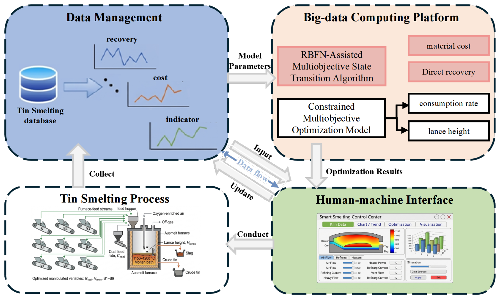
To address these gaps, this study develops RAMOSTA, an RBFN-assisted dynamic multiobjective state transition algorithm for tin-smelting parameter optimization. The proposed method is designed specifically for the limited-data, expensive-evaluation, and time-varying characteristics of the process. Radial basis function neural-network surrogate models are constructed to approximate tin recovery, energy consumption, and refractory-lining degradation based on the three adjustable parameters. The surrogate models reduce the number of costly direct evaluations required during the optimization process. An uncertainty-aware adaptive offset penalty is introduced to provide conservative constraint handling. The penalty margin is adjusted according to the uncertainty of the surrogate prediction and the constraint status, so that solutions with uncertain feasibility are treated more cautiously. A Pareto-based dynamic state-transition search strategy is then used to explore time-varying trade-offs among the three conflicting objectives while adapting the search to changes in the operating state. Finally, a hybrid-weight TOPSIS decision layer is developed to select an executable operating scheme from the obtained Pareto solutions. In this layer, the fuzzy analytic hierarchy process (FAHP) is used to represent expert preferences while accounting for the uncertainty of expert judgments, whereas Shapley values are used to quantify the marginal contribution of each objective to the overall decision. An adaptive cosine-similarity gating mechanism regulates the relative influence of these two types of information before TOPSIS ranking.

The main contributions of this study are as follows:

• A problem-driven constrained multiobjective optimization formulation is established for tin smelting by jointly considering tin recovery, energy consumption, and magnesia–chrome refractory degradation. The decision variables are explicitly limited to the coal-consumption rate, lance height, and belt-scale feed rate, thereby ensuring consistency between the optimization model and the actual adjustable operating parameters.
• An RBFN-assisted data-efficient evaluation mechanism is developed for the proposed optimization framework. The mechanism approximates the three process objectives using limited industrial data and reduces the number of expensive direct evaluations required during multiobjective search.
• An uncertainty-aware adaptive offset penalty mechanism is proposed for conservative constraint handling. The penalty margin is adjusted according to surrogate uncertainty and constraint violation information, reducing the risk of accepting solutions that appear feasible according to inaccurate surrogate predictions but may be unreliable in actual furnace operation.
• A dynamic state-transition search strategy is developed to capture the time-varying effects of the three adjustable parameters. The method considers the effects of the coal-consumption rate on thermal input, the lance height on gas dispersion and bath mixing, and the belt-scale feed rate on material loading and slag formation, thereby searching for operating trade-offs under changing furnace states rather than assuming a single static optimum.
• A hybrid decision-support procedure is developed to select an executable operating scheme from the Pareto set. FAHP is used to represent expert preferences under judgment uncertainty, while Shapley values quantify the marginal contribution of each objective. The adaptive cosine-similarity gating mechanism integrates these two types of decision information before TOPSIS ranking, providing an interpretable link between Pareto optimization and plant-oriented operating decisions.
• The proposed framework is evaluated using an industrial tin-smelting dataset and compared with NSGA-II, NSGA-III, MOEA/D, and C-TAEA. The evaluation considers Pareto-front quality, hypervolume, inverted generational distance, and constraint satisfaction, as well as the practical characteristics of the selected operating scheme.

The remainder of this paper is organized as follows. Section 2 describes the tin-smelting process and the three adjustable operating parameters, defines the constrained time-varying multiobjective optimization problem, and presents the RBFN surrogate models, uncertainty-aware adaptive offset penalty, dynamic state-transition search strategy, and hybrid-weight TOPSIS decision procedure. Section 3 reports the surrogate-model validation, comparative optimization results, constraint-satisfaction analysis, ablation studies, sensitivity analysis, and evaluation of the selected operating scheme using the industrial dataset. Section 4 discusses the optimization performance, the role of each methodological component, the industrial implications, and the limitations associated with offline surrogate-assisted validation. Finally, Section 5 summarizes the main findings and outlines future work, including uncertainty calibration, online surrogate updating, and prospective industrial validation.

2. Dynamic Multiobjective Optimization and Decision-Making Framework for Tin Smelting

2.1. Tin-Smelting Process and Control Variables

The tin-smelting process considered in this study is a top-blowing reduction and separation process involving gas, liquid, and solid phases. The process includes the reduction of tin-bearing oxides, slag formation, phase separation, heat transfer, and impurity removal under high-temperature conditions. The overall reduction relationship can be represented by

$${\mathrm{SnO}}_2+2\mathrm{C}\to \mathrm{Sn}+2\mathrm{CO}\uparrow$$

(1)

where the equation represents the principal reduction relationship rather than a complete description of the multiphase reaction mechanism. Other reactions involving iron oxides, silica, carbon monoxide, slag components, and minor impurity-bearing phases may occur simultaneously. These reactions affect the reduction environment, slag properties, heat transfer, impurity removal, and degradation of the magnesia–chrome refractory bricks lining the molten pool.

The manipulated variables were selected through field investigation at the cooperating tin-smelting plant. They represent operating parameters that can be directly adjusted by the operator or the plant control system within predefined equipment, production, and safety limits. The selected variables include the coal feed rate, lance height, and the feed rates of nine belt-scale systems. The coal feed rate affects the reducing-agent supply and the thermal input associated with carbon oxidation. The lance height, defined as the vertical distance from the lance tip to the molten-bath surface, affects the gas-jet penetration condition, gas–liquid interaction distance, bath agitation, and heat and mass transfer near the molten bath. The nine belt-scale feed rates determine the total amount and blending proportions of the confidential furnace-feed streams.

Although the identities and detailed compositions of the nine feed streams are not disclosed because of industrial confidentiality, the streams have different material characteristics and therefore make different contributions to the overall furnace burden. Their feed rates influence the effective burden composition through the weighted blending of the individual streams. In general, for a material property or component k, the effective burden value can be conceptually expressed as

$${\overline{z}}_k\left(t\right)={\displaystyle \frac{{\displaystyle {\displaystyle \sum _{j=1}^9}{B}_j\left(t\right)z_{jk}}}{{\displaystyle {\displaystyle \sum _{j=1}^9}{B}_j\left(t\right)}}},$$

(2)

where $B_j\left(t\right)$ is the feed rate of the jth belt-scale stream and $z_{jk}$ denotes the corresponding, confidential material property or component fraction. The values of $z_{jk}$ are not reported in this paper. Equation (2) is introduced only to describe the blending mechanism and does not disclose the identity or detailed composition of any individual feed stream.

The resulting effective burden composition and total feed rate influence the slag condition through several process-level mechanisms. First, they affect the loading of slag-forming components and consequently the amount of slag generated during smelting. Second, they modify the relative proportion of oxide components in the burden and may therefore change the effective acidity–basicity balance, liquidus-temperature tendency, liquid-phase fraction, and apparent slag viscosity. Third, changes in the amount of reducible material and other burden components influence the thermal demand and reduction environment required to maintain the desired smelting condition. These changes may further affect slag fluidity, gas–liquid–solid mixing, the settling and separation of metal and slag phases, and the transfer or retention of tin between the slag and metal phases. Therefore, the nine belt-scale feed rates do not influence the slag merely by changing the feed quantity; they also change the effective composition and physicochemical condition of the slag-forming system. In turn, the altered slag condition affects tin recovery, energy consumption, and the chemical and mechanical interaction between the molten slag and the magnesia–chrome refractory lining.

The control vector is defined as

$$\mathit{u}\left(t\right)={\left[G_{\mathrm{coal}}\left(t\right),H_{\mathrm{lance}}\left(t\right),B_1\left(t\right),B_2\left(t\right),\dots ,B_9\left(t\right)\right]}^{\mathrm{T}},$$

(3)

where $G_{\mathrm{coal}}\left(t\right)$ denotes the plant-level coal feed rate, $H_{\mathrm{lance}}\left(t\right)$ denotes the vertical distance from the lance tip to the molten-bath surface, and $B_j\left(t\right)$ denotes the feed rate measured by the jth belt scale, $j=1,\dots ,9$. The nine belt scales correspond to confidential furnace-feed streams with different material characteristics. Their detailed identities, compositions, and numerical operating ranges are not disclosed because of industrial confidentiality.

When coal-bearing material is delivered through one or more of the belt-scale systems, $G_{\mathrm{coal}}\left(t\right)$ represents the corresponding aggregate coal feed rate used for the thermal and reduction calculations. In this case, the aggregate coal rate is calculated consistently from the relevant belt-scale measurements and is not independently varied in a manner that would double-count the same material input. Thus, the optimization variables are limited to the plant-adjustable coal-feed condition, lance height, and belt-scale feed rates.

The feasible range of each manipulated variable is determined by equipment capacity, material-feeding capability, standard operating procedures, and safety requirements. The control vector includes only variables that are directly adjustable during plant operation. Measured furnace conditions, feed characteristics that are not directly adjustable, and external disturbances are treated as state variables or contextual variables rather than as manipulated variables.

The reduced process-state vector is defined as

$$\mathit{x}\left(t\right)={\left[C_{{\mathrm{Sn}}^{2+}}\left(t\right),T\left(t\right),C_{{\mathrm{O}}_2}\left(t\right),H\left(t\right)\right]}^{\mathrm{T}},$$

(4)

where $C_{{\mathrm{Sn}}^{2+}}\left(t\right)$ represents the tin-related process state, $T\left(t\right)$ is the furnace-temperature state, $C_{{\mathrm{O}}_2}\left(t\right)$ is the gas-phase oxygen-related state, and $H\left(t\right)$ represents the effective thermal state. These state variables are obtained from process measurements when available and are otherwise propagated through the reduced state-transition model.

For computational efficiency, the furnace is represented by a reduced material–energy balance model. This model is used to propagate the furnace-state trajectory and to evaluate state-related operating constraints. It does not replace direct plant measurements and does not attempt to reproduce every detailed chemical reaction, equilibrium relationship, or transport phenomenon occurring in the furnace. Its compact form is

$$\dot{\mathit{x}}\left(t\right)=\Gamma \left(\mathit{x}\left(t\right),\mathit{u}\left(t\right),t\right),\mathit{x}\left(t_0\right)={\mathit{x}}_0.$$

(5)

Within the reduced state-transition model, the effects of the nine belt-scale feed rates are represented through their contributions to the total material input, effective burden composition, reducible-material loading, thermal demand, and slag-forming-material loading. The slag-related terms in $\Gamma (·)$ therefore represent the process-level consequences of feed-rate changes, including changes in slag generation, effective slag condition, phase-separation behavior, and tin distribution between the slag and metal phases. This reduced representation captures the influence of the controllable feed streams without attempting to reconstruct the complete equilibrium composition or detailed multiphase transport field of the industrial furnace.

The effective combustion heat generation is represented by

$$P_{\mathrm{comb}}\left(t\right)={\eta }_{\mathrm{comb}}\Delta H_{\mathrm{C}}{G}_{\mathrm{coal}}\left(t\right),$$

(6)

where ${\eta }_{\mathrm{comb}}$ denotes the effective combustion efficiency and $\Delta H_{\mathrm{C}}$ denotes the effective heat-release coefficient associated with carbon oxidation. The material-feeding variables $B_1\left(t\right),\dots ,B_9\left(t\right)$ affect the state-transition model through the material-balance, effective-burden, thermal-load, reducible-material-loading, and slag-condition terms contained in $\Gamma (·)$.

The mechanistic component is used for state propagation and state-related constraint checking. Three radial basis function network (RBFN) models are used separately to predict tin direct recovery, energy consumption, and magnesia–chrome refractory degradation. Therefore, the proposed method is a sequential mechanism-assisted and data-driven optimization framework, rather than a fully coupled hybrid model with jointly trained mechanistic and neural components. The effective coefficients in the reduced state model are calibrated using plant process information and are not disclosed because of industrial confidentiality.

2.2. Problem Formulation

The operating parameters are optimized over a finite production horizon to account for the time-varying furnace state and the effects of the operating schedule. In this study, the manipulated variables are limited to the coal feed rate, lance height, and the feed rates of the nine belt-scale systems. The furnace state evolves with these operating variables, and a control action applied at one time interval may influence the thermal condition, material loading, slag condition, and feasible operating region in subsequent intervals. Feed characteristics that cannot be directly adjusted and other external disturbances are treated as contextual variables or sources of process uncertainty rather than as manipulated variables. Because repeated high-fidelity simulation and real-plant trials are expensive, the objective functions are evaluated using surrogate models trained from historical plant data.

The RBFN surrogate input vector consists only of the directly adjustable operating variables. It includes one coal feed rate, one lance height, and nine belt-scale feed rates. Therefore, the surrogate input dimension is $d=11$ and is defined as

$$\mathit{\xi }\left(t\right)=\mathit{u}\left(t\right)={\left[G_{\mathrm{coal}}\left(t\right),H_{\mathrm{lance}}\left(t\right),B_1\left(t\right),B_2\left(t\right),\dots ,B_9\left(t\right)\right]}^{\mathrm{T}}.$$

(7)

Here, $G_{\mathrm{coal}}\left(t\right)$ denotes the coal feed rate, $H_{\mathrm{lance}}\left(t\right)$ denotes the vertical distance from the lance tip to the molten-bath surface, and $B_j\left(t\right)$ denotes the feed rate of the jth belt-scale system, with $j=1,\dots ,9$. The reduced furnace-state vector $\mathit{x}\left(t\right)$ is not included as an independent input of the RBFN models. Instead, it is propagated separately by the reduced state-transition model and is used for furnace-state constraint checking and for describing the dynamic process context.

Let $t_0$ and $t_f$ denote the start and end of the optimization horizon, respectively. Three conflicting objectives are considered.

The first objective is to maximize the average direct recovery of tin. Since the optimization algorithm is implemented in minimization form, the negative recovery is minimized:

$$F_1=-\overline{R},\overline{R}={\displaystyle \frac{1}{t_f-t_0}}{\int }_{t_0}^{t_f}\widehat{R}\left(\mathit{\xi }\left(t\right)\right)dt.$$

(8)

The second objective is to minimize the average energy-consumption index:

$$F_2=\overline{E}={\displaystyle \frac{1}{t_f-t_0}}{\int }_{t_0}^{t_f}\widehat{E}\left(\mathit{\xi }\left(t\right)\right)dt.$$

(9)

The third objective is to minimize the average predicted refractory-degradation burden:

$$F_3={\overline{Q}}_{\mathrm{ref}}={\displaystyle \frac{1}{t_f-t_0}}{\int }_{t_0}^{t_f}{\widehat{Q}}_{\mathrm{ref}}\left(\mathit{\xi }\left(t\right)\right)dt.$$

(10)

In this study, $Q_{\mathrm{ref}}\left(t\right)$ denotes a dimensionless refractory-degradation index for the magnesia–chrome refractory lining in the molten-pool region. It is used to quantify the predicted degradation burden imposed on the refractory lining under the evaluated operating condition. The index is constructed from refractory-related process information and operating-condition information available from the cooperating plant, including the effects associated with high-temperature exposure, thermal gradients, slag–metal interaction, and mechanical erosion. A higher value of $Q_{\mathrm{ref}}\left(t\right)$ indicates a greater predicted degradation burden and therefore a less favorable refractory-service condition. The index is normalized within the modeling and optimization procedure so that it can be compared across operating schedules without disclosing confidential plant-specific measurement units, coefficients, or calibration details.

The refractory-degradation index is not interpreted as a direct instantaneous measurement of refractory thickness loss. Instead, it is an empirical process-performance indicator that represents the relative refractory-degradation burden under the evaluated operating condition. Its dependence on the manipulated variables is learned by the RBFN model from historical plant data. At the process level, the coal feed rate may affect the refractory burden through changes in heat input and temperature gradients; the lance height may affect it through changes in gas-jet penetration, bath agitation, local turbulence, and slag–metal interaction; and the nine belt-scale feed rates may affect it through changes in material loading, effective burden composition, slag generation, slag fluidity, and contact between the molten phases and the refractory lining.

Although the furnace-state vector $\mathit{x}\left(t\right)$ is not used as an independent RBFN input, it is propagated by the reduced state-transition model to evaluate the dynamic evolution and state-related constraints of the furnace. The state trajectory provides the process context for the operating schedule, whereas the RBFN models directly map the 11-dimensional manipulated-variable vector $\mathit{\xi }\left(t\right)=\mathit{u}\left(t\right)$ to the three process-response predictions.

Here, $\widehat{R}(·)$, $\widehat{E}(·)$, and ${\widehat{Q}}_{\mathrm{ref}}(·)$ denote the RBFN predictions of direct tin recovery, energy consumption, and the normalized magnesia–chrome refractory-degradation index, respectively. Therefore, $F_3$ represents the average predicted refractory-degradation burden over the optimization horizon, rather than an additional physical measurement or an independent optimization variable. Minimizing $F_3$ favors operating schedules that reduce the cumulative exposure of the refractory lining to unfavorable thermal, chemical, and mechanical conditions.

The operating variables are constrained by equipment capability, feeder capacity, lance-adjustment limits, and standard operating procedures:

$${\mathit{u}}_{\mathrm{lb}}\le \mathit{u}\left(t\right)\le {\mathit{u}}_{\mathrm{ub}},t\in [t_0,t_f].$$

(11)

The control vector is given by

$$\mathit{u}\left(t\right)={\left[G_{\mathrm{coal}}\left(t\right),H_{\mathrm{lance}}\left(t\right),B_1\left(t\right),B_2\left(t\right),\dots ,B_9\left(t\right)\right]}^{\mathrm{T}},$$

(12)

where $G_{\mathrm{coal}}\left(t\right)$ denotes the coal feed rate, $H_{\mathrm{lance}}\left(t\right)$ denotes the vertical distance from the lance tip to the molten-bath surface, and $B_j\left(t\right)$ denotes the feed rate of the jth belt-scale system, with $j=1,\dots ,9$. The nine belt-scale systems correspond to confidential furnace-feed streams with different material characteristics. Their detailed material identities, compositions, and numerical operating ranges are not disclosed because of industrial confidentiality.

The main predicted process responses are restricted to their acceptable operating regions:

$$\begin{array}{cc}\hfill R_{\mathrm{lb}}& \le \widehat{R}\left(\mathit{\xi }\left(t\right)\right)\le R_{\mathrm{ub}},\hfill \\ \hfill E_{\mathrm{lb}}& \le \widehat{E}\left(\mathit{\xi }\left(t\right)\right)\le E_{\mathrm{ub}},\hfill \\ \hfill Q_{\mathrm{ref},\mathrm{lb}}& \le {\widehat{Q}}_{\mathrm{ref}}\left(\mathit{\xi }\left(t\right)\right)\le Q_{\mathrm{ref},\mathrm{ub}}.\hfill \end{array}$$

(13)

The bounds on R, E, and $Q_{\mathrm{ref}}$ represent plant-specific acceptable regions. In particular, the upper bound on $Q_{\mathrm{ref}}$ limits the predicted refractory-degradation burden, whereas the bounds on recovery and energy consumption prevent the optimization from obtaining apparently favorable refractory conditions by sacrificing essential production or energy-performance requirements.

The furnace-state constraints are expressed as

$$T_{min}\le T\left(t\right)\le T_{max},C_{\mathrm{resid}}^{\mathrm{Sn}}\left(t\right)\le C_{\mathrm{target}},T\left(t_f\right)=T_{\mathrm{set}}.$$

(14)

Here, $T\left(t\right)$ denotes the furnace-temperature state, $C_{\mathrm{resid}}^{\mathrm{Sn}}\left(t\right)$ denotes the residual tin-related concentration or residual tin indicator used for process control, and $T_{\mathrm{set}}$ is the desired terminal furnace-temperature state. These quantities are evaluated from available process information and the reduced state-transition model. Their detailed plant-specific definitions and numerical limits are not disclosed because of industrial confidentiality.

The safety margin is used only as a constraint-handling mechanism. It is not treated as an additional optimization objective and is not included in the objective vector. During optimization, an uncertainty-dependent offset is added to the nominal constraint function to reduce the risk that a candidate solution is accepted because of surrogate prediction error. In particular, when the prediction uncertainty of $\widehat{R}$, $\widehat{E}$, or ${\widehat{Q}}_{\mathrm{ref}}$ is large, the corresponding feasible region is treated more conservatively. The original equipment, thermal, product-quality, energy-performance, and refractory-related limits remain the physical acceptance criteria. Thus, the tightened constraints are used to guide the search conservatively, whereas final feasibility is assessed against the original plant limits.

The complete constrained dynamic multiobjective optimization problem is formulated as

$$\begin{array}{cc}\hfill \underset{\mathit{u}\left(t\right)}{min}& \mathit{F}(\mathit{u},t)={[F_1,F_2,F_3]}^{\mathrm{T}},\hfill \\ \hfill \mathrm{s}.\mathrm{t}.& \dot{\mathit{x}}\left(t\right)=\Gamma (\mathit{x}\left(t\right),\mathit{u}\left(t\right),t),\hfill \\ \hfill & \mathit{x}\left(t_0\right)={\mathit{x}}_0,\hfill \\ \hfill & {\mathit{u}}_{\mathrm{lb}}\le \mathit{u}\left(t\right)\le {\mathit{u}}_{\mathrm{ub}},\hfill \\ \hfill & R_{\mathrm{lb}}\le \widehat{R}\left(\mathit{\xi }\left(t\right)\right)\le R_{\mathrm{ub}},\hfill \\ \hfill & E_{\mathrm{lb}}\le \widehat{E}\left(\mathit{\xi }\left(t\right)\right)\le E_{\mathrm{ub}},\hfill \\ \hfill & Q_{\mathrm{ref},\mathrm{lb}}\le {\widehat{Q}}_{\mathrm{ref}}\left(\mathit{\xi }\left(t\right)\right)\le Q_{\mathrm{ref},\mathrm{ub}},\hfill \\ \hfill & T_{min}\le T\left(t\right)\le T_{max},\hfill \\ \hfill & C_{\mathrm{resid}}^{\mathrm{Sn}}\left(t\right)\le C_{\mathrm{target}},\hfill \\ \hfill & T\left(t_f\right)=T_{\mathrm{set}},t\in [t_0,t_f].\hfill \end{array}$$

(15)

The objective vector therefore contains three process-level performance criteria: the negative average direct tin recovery, the average energy-consumption index, and the average normalized refractory-degradation burden. The optimization directly regulates only the 11 manipulated variables, namely, the coal feed rate, lance height, and nine belt-scale feed rates. The furnace-state trajectory is determined separately by the reduced state-transition model, and the effects of the manipulated variables on furnace-state evolution, effective burden condition, slag behavior, and refractory degradation are represented through the state model, the process constraints, and the RBFN surrogate models.

The numerical operating limits, normalization parameters, refractory-index construction details, and plant-specific calibration coefficients are maintained internally and are not disclosed because of industrial confidentiality. The reported optimization results are therefore interpreted in terms of normalized process indicators and relative performance comparisons among feasible operating schedules.

2.3. RBFN-Based Surrogate Modeling

The surrogate models are constructed to approximate the three process responses associated with the plant-adjustable operating variables. In accordance with the process description in Section 2.1, the input vector contains only the coal feed rate, the lance height, and the feed rates of the nine belt-scale systems. Therefore, the input dimension of the RBFN surrogate models is $d=11$. The four reduced furnace-state variables are propagated separately by the reduced state-transition model and are used for furnace-state constraint checking; they are not included as independent inputs of the RBFN response models.

The 11-dimensional surrogate input vector is defined as

$$\mathit{\xi }\left(t\right)=\mathit{u}\left(t\right)={\left[G_{\mathrm{coal}}\left(t\right),H_{\mathrm{lance}}\left(t\right),B_1\left(t\right),B_2\left(t\right),\dots ,B_9\left(t\right)\right]}^{\mathrm{T}},$$

(16)

where $G_{\mathrm{coal}}\left(t\right)$ denotes the coal feed rate, $H_{\mathrm{lance}}\left(t\right)$ denotes the lance height, and $B_j\left(t\right)$ denotes the feed rate of the jth belt-scale system, with $j=1,\dots ,9$. Thus, the surrogate models use only the directly adjustable operating variables. The furnace-state trajectory $\mathit{x}\left(t\right)$ is calculated separately from the reduced state-transition model and is used to evaluate state-related constraints and to describe the dynamic process context.

Before model training, each of the 11 input variables and each output variable is transformed into a normalized representation. The normalization parameters are calculated only from the training subset and are then reused without modification for the validation subset, test subset, and optimization procedure. This treatment prevents information from the validation or test periods from entering the data-preprocessing stage. Missing observations are imputed using the median of the corresponding variable calculated from the training subset. Potential abnormal observations are screened using the interquartile-range rule and are removed only when they are confirmed to be measurement or recording errors. Observations that are statistically unusual but physically plausible are retained as valid process samples because they may represent actual operating conditions. The available observations are divided chronologically into training, validation, and test subsets. The chronological division is used to prevent information leakage from later production periods and to provide a more realistic evaluation of the ability of the surrogate models to generalize to subsequent operating conditions.

For a response variable y, the normalized root mean squared error (RMSE) on a dataset $\mathcal{D}$ is calculated as

$${RMSE}_{\mathcal{D}}=\sqrt{{\displaystyle \frac{1}{\left|\mathcal{D}\right|}}{\sum }_{i\in \mathcal{D}}{\left(y_i-{\widehat{y}}_i\right)}^2},$$

(17)

where $\left|\mathcal{D}\right|$ denotes the number of samples in the corresponding dataset, $y_i$ is the normalized measured or assessed response, and ${\widehat{y}}_i$ is the normalized RBFN prediction. The validation RMSE is calculated using observations that are not used to estimate the output-layer weights. It therefore provides an independent error measure for model development and hyperparameter selection. The test RMSE is calculated only after the model structure and all hyperparameters have been fixed.

An RBFN represents a nonlinear mapping from the 11-dimensional operating-variable vector to a process response by a weighted sum of radially symmetric basis functions:

$$\widehat{y}\left(\mathit{\xi }\right)={\displaystyle \sum _{j=1}^M}{w}_j\varphi \left({\displaystyle \frac{{∥\mathit{\xi }-{\mathit{c}}_j∥}_2}{{\sigma }_j}}\right)+b,$$

(18)

where M is the number of basis functions, ${\mathit{c}}_j$ and ${\sigma }_j$ are the center and width of the jth basis function, respectively, and $w_j$ and b are the output weight and bias. A Gaussian kernel is used:

$$\varphi \left(r\right)=exp(-r^2).$$

(19)

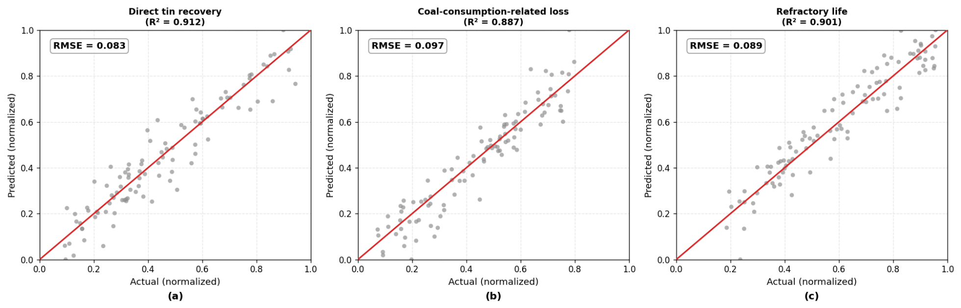
Three independent RBFN models are trained for direct tin recovery, energy consumption, and the normalized magnesia–chrome refractory-degradation index. The models are trained separately because the three responses have different process meanings, scales, and error characteristics. The use of independent response models also allows the prediction error of each objective to be evaluated separately.

The RBF centers are selected by applying k-means++ clustering to the 11-dimensional training inputs. The clustering procedure is performed using the training subset only. Candidate values of the number of centers are evaluated using the validation subset. For each response model, the center number is selected by comparing the validation RMSE values obtained under the predefined candidate configurations. The model with the smallest validation RMSE is not selected because of its training fit; rather, it is selected because it provides the smallest prediction error on previously unused chronological validation observations among the candidate models. This criterion helps to balance approximation accuracy and generalization performance. In contrast, selecting a model according to the minimum training RMSE could favor an unnecessarily complex model and increase the risk of overfitting.

The initial RBF width is determined from the median nearest-center distance. This quantity provides a data-dependent reference scale for the local spacing of the RBF centers. Specifically, if $d_j^{\mathrm{near}}$ denotes the distance between center ${\mathit{c}}_j$ and its nearest other center, the reference width is defined as

$${\sigma }_0=\sqrt{2}median\left\{d_j^{\mathrm{near}}:j=1,\dots ,M\right\}.$$

(20)

Three candidate width values are considered:

$$\sigma \in \left\{0.5{\sigma }_0,{\sigma }_0,2{\sigma }_0\right\}.$$

(21)

The factor $0.5$ produces narrower basis functions and more local approximation behavior. The factor 1 retains the width determined from the center distribution. The factor 2 produces wider basis functions and smoother approximation behavior. This validation grid examines the trade-off between local fitting and smooth generalization without introducing an excessively large hyperparameter-search cost.

Once a candidate number of centers and width have been specified, the RBF activation matrix for the training samples is constructed as

$${\mathsf{\Phi }}_{\mathrm{tr}}=\left[\begin{array}{cccc}{\varphi }_{1,1}& {\varphi }_{1,2}& \cdots & {\varphi }_{1,M}\\ {\varphi }_{2,1}& {\varphi }_{2,2}& \cdots & {\varphi }_{2,M}\\ ⋮& ⋮& \ddots & ⋮\\ {\varphi }_{N_{\mathrm{tr}},1}& {\varphi }_{N_{\mathrm{tr}},2}& \cdots & {\varphi }_{N_{\mathrm{tr}},M}\end{array}\right],$$

(22)

where

$${\varphi }_{i,j}=\varphi \left({\displaystyle \frac{{∥{\mathit{\xi }}_i-{\mathit{c}}_j∥}_2}{\sigma }}\right).$$

(23)

The bias term is included by augmenting the activation matrix with a column of ones. The output-layer weights are estimated using ridge-regularized linear least squares:

$$\widehat{\beta }=arg\underset{\beta }{min}\left\{{∥{\mathit{y}}_{\mathrm{tr}}-{\tilde{\mathsf{\Phi }}}_{\mathrm{tr}}\beta ∥}_2^2+\lambda {∥{\beta }_{\mathrm{w}}∥}_2^2\right\},$$

(24)

where ${\tilde{\mathsf{\Phi }}}_{\mathrm{tr}}$ is the activation matrix augmented with the bias column, $\beta$ contains the output weights and bias, ${\beta }_{\mathrm{w}}$ contains only the output weights, and $\lambda$ is the ridge coefficient. The bias is not penalized.

Ridge regularization is adopted because adjacent Gaussian basis functions may overlap substantially, which can produce correlated columns in the RBF activation matrix. This issue is particularly relevant when the industrial dataset is limited and contains measurement noise or correlated operating variables. The ridge term stabilizes weight estimation, reduces weight variance, and limits overfitting while preserving the computational efficiency of linear output-layer training.

For each response model, the candidate number of centers, width factor, and ridge coefficient are selected jointly using the chronological validation RMSE. Let $\mathcal{H}$ denote the predefined set of candidate hyperparameter combinations. The selected configuration is defined as

$${\mathit{h}}^{*}=arg\underset{\mathit{h}\in \mathcal{H}}{min}{RMSE}_{\mathrm{val}}\left(\mathit{h}\right),$$

(25)

where $\mathit{h}=(M,\sigma ,\lambda )$ represents one candidate RBFN configuration. The minimum validation RMSE is used because it selects the candidate configuration with the smallest prediction error on the independent chronological validation period. This criterion is more appropriate than the training RMSE for model selection because the training RMSE may decrease as model complexity increases, even when the generalization performance deteriorates. The validation RMSE therefore provides a practical criterion for balancing fitting accuracy, model complexity, and prediction performance on subsequent operating periods.

After ${\mathit{h}}^{*}$ is selected, the corresponding model is evaluated once on the untouched chronological test subset. The test RMSE, together with other error measures reported in Section 3, is used to assess the out-of-sample predictive performance of the final surrogate model. The test subset is not used to select the center number, width, ridge coefficient, normalization parameters, or model structure. No model setting is adjusted according to the test results.

The initial algorithmic configuration is summarized in

Table 1. Initial configuration and validation procedure of the RBFN surrogate models.

Item	Initial Setting
Input dimension	$d=11$
Input variables	1 coal feed rate, 1 lance height, 9 belt-scale feed rates
Output variables	$\widehat{R}$, $\widehat{E}$, and ${\widehat{Q}}_{\mathrm{ref}}$
Kernel	Gaussian, $\varphi \left(r\right)=exp(-r^2)$
Center selection	k-means++ using the training subset
Candidate center numbers	$M\in \{10,20,30,40,60\}$
Initial width	Median nearest-center distance multiplied by $\sqrt{2}$
Width candidates	$\{0.5,1,2\}$ times the initial width
Weight estimation	Ridge-regularized least squares
Ridge candidates	$\{{10}^{-8},{10}^{-6},{10}^{-4},{10}^{-2}\}$
Hyperparameter selection	Minimum chronological validation RMSE
Final performance assessment	Untouched chronological test subset
Bootstrap members	$B=5$ for uncertainty estimation

. These values are surrogate-model settings rather than confidential plant operating data.

To estimate predictive uncertainty for constraint handling, $B=5$ bootstrap RBFN members are constructed for each response. Each member is trained using a bootstrap resample of the training subset, while the chronological validation and test subsets remain untouched. For an input $\mathit{\xi }$, the ensemble prediction is calculated as

$$\overline{y}\left(\mathit{\xi }\right)={\displaystyle \frac{1}{B}}{\displaystyle \sum _{b=1}^B}{\widehat{y}}^{\left(b\right)}\left(\mathit{\xi }\right),$$

(26)

and the corresponding empirical predictive dispersion is estimated by

$$s_y\left(\mathit{\xi }\right)=\sqrt{{\displaystyle \frac{1}{B-1}}\sum _{b=1}^B{\left[{\widehat{y}}^{\left(b\right)}\left(\mathit{\xi }\right)-\overline{y}\left(\mathit{\xi }\right)\right]}^2}.$$

(27)

The ensemble mean is used as the nominal prediction, whereas $s_y\left(\mathit{\xi }\right)$ is used as an empirical measure of model-disagreement uncertainty in the uncertainty-aware adaptive offset penalty. This uncertainty measure is intended to support conservative constraint handling; it is not interpreted as a complete probabilistic confidence interval for the industrial process.

For the three response models, the nominal predicted outputs are denoted by $\widehat{R}\left(\mathit{\xi }\right)$, $\widehat{E}\left(\mathit{\xi }\right)$, and ${\widehat{Q}}_{\mathrm{ref}}\left(\mathit{\xi }\right)$, respectively. Here, ${\widehat{Q}}_{\mathrm{ref}}\left(\mathit{\xi }\right)$ denotes the predicted normalized magnesia–chrome refractory-degradation burden rather than a direct instantaneous measurement of refractory thickness loss. During candidate evaluation, the reduced state model propagates the furnace-state trajectory for a proposed schedule of the 11 operating variables. The RBFN models predict the corresponding process responses from the 11-dimensional operating-variable input. The predicted responses are aggregated over the optimization horizon to calculate the three objective values, while the state constraints are evaluated separately using the propagated state trajectory. The final surrogate performance is assessed using the chronological test subset before the models are used in the optimization procedure.

2.4. Dynamic Multiobjective State Transition Optimization

The control trajectory is represented by a piecewise-constant schedule:

$$\mathit{U}=[{\mathit{u}}_1,{\mathit{u}}_2,\dots ,{\mathit{u}}_{N_t}],\mathit{u}\left(t\right)={\mathit{u}}_k,t\in [t_{k-1},t_k).$$

(28)

Each control vector contains the eleven directly adjustable operating variables:

$${\mathit{u}}_k={\left[G_{\mathrm{coal},k},H_{\mathrm{lance},k},B_{1,k},B_{2,k},\dots ,B_{9,k}\right]}^{\mathrm{T}}\in {\mathbb{R}}^{11}.$$

(29)

Here, $G_{\mathrm{coal},k}$ denotes the coal feed rate, $H_{\mathrm{lance},k}$ denotes the lance height, and $B_{j,k}$ denotes the feed rate of the jth belt-scale system. Thus, each candidate solution represents a complete schedule for one coal feed rate, one lance height, and nine belt-scale feed rates over the considered production horizon. The values of $N_t$, the horizon length, and the control-interval duration are specified in the experimental protocol without disclosing confidential plant time scales.

For the search operators, the schedule is vectorized as

$$vec\left(\mathit{U}\right)={\left[{\mathit{u}}_1^{\mathrm{T}},{\mathit{u}}_2^{\mathrm{T}},\dots ,{\mathit{u}}_{N_t}^{\mathrm{T}}\right]}^{\mathrm{T}}\in {\mathbb{R}}^n,n=11N_t.$$

(30)

The RBFN surrogate input at each control interval is the eleven-dimensional operating-variable vector

$${\mathit{\xi }}_k={\mathit{u}}_k={\left[G_{\mathrm{coal},k},H_{\mathrm{lance},k},B_{1,k},\dots ,B_{9,k}\right]}^{\mathrm{T}}.$$

(31)

The reduced furnace-state vector $\mathit{x}\left(t\right)$ is propagated separately using the reduced state-transition model. It is not included as an independent RBFN input. Instead, it is used for dynamic state propagation, state-related constraint evaluation, and a description of the evolving furnace condition.

A Pareto archive is maintained during the optimization process. Candidate schedules are generated using rotation, translation, expansion, and axesion operators. The operators are mathematical search-space transformations; they do not represent physical rotation or movement of the furnace equipment. After each transformation, the candidate schedule is projected onto the admissible bounds of the eleven manipulated variables.

For a current candidate schedule ${\mathit{U}}_k$, the rotation operator is expressed as

$$vec\left({\mathit{U}}_{k+1}\right)=vec\left({\mathit{U}}_k\right)+{\displaystyle \frac{\alpha }{n{∥vec\left({\mathit{U}}_k\right)∥}_2}}{\mathit{R}}_{r}vec\left({\mathit{U}}_k\right),$$

(32)

where $n=11N_t$ is the dimension of the vectorized schedule, $\alpha$ is the rotation factor, and ${\mathit{R}}_r$ is a random matrix whose entries are sampled from a bounded uniform distribution. The rotation operator changes the direction and magnitude of the current schedule vector in the normalized decision space. It creates a perturbed schedule that may differ simultaneously across multiple control intervals and control variables. Thus, the term “rotation” refers to a directional search transformation in the normalized decision space, rather than to a physical rotation of the lance.

The translation operator generates a candidate along the direction from the preceding schedule ${\mathit{U}}_{k-1}$ to the current schedule ${\mathit{U}}_k$:

$$vec\left({\mathit{U}}_{k+1}\right)=vec\left({\mathit{U}}_k\right)+\beta R_t{\displaystyle \frac{vec\left({\mathit{U}}_k\right)-vec\left({\mathit{U}}_{k-1}\right)}{{∥vec\left({\mathit{U}}_k\right)-vec\left({\mathit{U}}_{k-1}\right)∥}_2+\epsilon }},$$

(33)

where $\beta$ is the translation factor, $R_t\in [0,1]$ is a random scalar, and $\epsilon$ is a small positive constant that prevents division by zero.

The expansion operator is defined as

$$vec\left({\mathit{U}}_{k+1}\right)=vec\left({\mathit{U}}_k\right)+\gamma {\mathit{R}}_{e}vec\left({\mathit{U}}_k\right),$$

(34)

where $\gamma$ is the expansion factor and ${\mathit{R}}_e$ is a diagonal Gaussian random matrix. This operator enables a larger-scale exploration of the search space.

The axesion operator is defined as

$$vec\left({\mathit{U}}_{k+1}\right)=vec\left({\mathit{U}}_k\right)+\delta {\mathit{R}}_{a}vec\left({\mathit{U}}_k\right),$$

(35)

where $\delta$ is the axesion factor and ${\mathit{R}}_a$ is a diagonal random matrix with only one nonzero diagonal element. The axesion operator performs a single-direction perturbation and is used to refine an individual decision dimension of the vectorized schedule.

After each search transformation, the generated schedule is projected onto the admissible bounds of the eleven manipulated variables:

$$u_{\ell ,k}^{\mathrm{proj}}=min\left\{u_{\ell ,\mathrm{ub}},max\left\{u_{\ell ,\mathrm{lb}},u_{\ell ,k}\right\}\right\},\ell =1,\dots ,11,k=1,\dots ,N_t.$$

(36)

The projected schedule is then propagated through the reduced state-transition model:

$$\dot{\mathit{x}}\left(t\right)=\Gamma \left(\mathit{x}\left(t\right),\mathit{u}\left(t\right),t\right),\mathit{x}\left(t_0\right)={\mathit{x}}_0.$$

(37)

At each control interval, the three RBFN surrogate models are evaluated using the eleven-dimensional input ${\mathit{\xi }}_k={\mathit{u}}_k$. The resulting predictions are aggregated over the optimization horizon to calculate the nominal objective vector:

$$\mathit{F}\left(\mathit{U}\right)={\left[F_1\left(\mathit{U}\right),F_2\left(\mathit{U}\right),F_3\left(\mathit{U}\right)\right]}^{\mathrm{T}},$$

(38)

where $F_1$, $F_2$, and $F_3$ are the negative average direct tin recovery, the average energy-consumption index, and the average normalized magnesia–chrome refractory-degradation burden, respectively.

To make the constraint-handling procedure explicit, the violation of a scalar inequality constraint is defined using its positive-part operator:

$${\left[z\right]}_{+}=max(0,z).$$

(39)

For a predicted response $y\left(t\right)$ subject to

$$y_{\mathrm{lb}}\le \widehat{y}\left(t\right)\le y_{\mathrm{ub}},$$

the normalized violation is defined as

$$v_y\left(t\right)={\displaystyle \frac{{\left[y_{\mathrm{lb}}-\widehat{y}\left(t\right)\right]}_{+}}{s_y^{\mathrm{lb}}}}+{\displaystyle \frac{{\left[\widehat{y}\left(t\right)-y_{\mathrm{ub}}\right]}_{+}}{s_y^{\mathrm{ub}}}},$$

(40)

where $s_y^{\mathrm{lb}}$ and $s_y^{\mathrm{ub}}$ are positive scaling constants based on the corresponding acceptable ranges. The scaling prevents variables with different units or numerical magnitudes from dominating the total violation measure.

For the process-response constraints, the instantaneous nominal violation is

$$\begin{array}{cc}\hfill v_{\mathrm{resp}}\left(t\right)=& v_R\left(t\right)+v_E\left(t\right)+v_{Q_{\mathrm{ref}}}\left(t\right),\hfill \end{array}$$

(41)

where

$$\begin{array}{cc}\hfill v_R\left(t\right)=& {\displaystyle \frac{{\left[R_{\mathrm{lb}}-\widehat{R}\left(\mathit{\xi }\left(t\right)\right)\right]}_{+}}{s_R^{\mathrm{lb}}}}+{\displaystyle \frac{{\left[\widehat{R}\left(\mathit{\xi }\left(t\right)\right)-R_{\mathrm{ub}}\right]}_{+}}{s_R^{\mathrm{ub}}}},\hfill \\ \hfill v_E\left(t\right)=& {\displaystyle \frac{{\left[E_{\mathrm{lb}}-\widehat{E}\left(\mathit{\xi }\left(t\right)\right)\right]}_{+}}{s_E^{\mathrm{lb}}}}+{\displaystyle \frac{{\left[\widehat{E}\left(\mathit{\xi }\left(t\right)\right)-E_{\mathrm{ub}}\right]}_{+}}{s_E^{\mathrm{ub}}}},\hfill \\ \hfill v_{Q_{\mathrm{ref}}}\left(t\right)=& {\displaystyle \frac{{\left[Q_{\mathrm{ref},\mathrm{lb}}-{\widehat{Q}}_{\mathrm{ref}}\left(\mathit{\xi }\left(t\right)\right)\right]}_{+}}{s_{Q_{\mathrm{ref}}}^{\mathrm{lb}}}}+{\displaystyle \frac{{\left[{\widehat{Q}}_{\mathrm{ref}}\left(\mathit{\xi }\left(t\right)\right)-Q_{\mathrm{ref},\mathrm{ub}}\right]}_{+}}{s_{Q_{\mathrm{ref}}}^{\mathrm{ub}}}}.\hfill \end{array}$$

(42)

The manipulated-variable violation is calculated as

$$v_u\left(t\right)={\displaystyle \sum _{\ell =1}^{11}}{\left[{\displaystyle \frac{u_{\ell ,\mathrm{lb}}-u_{\ell }\left(t\right)}{s_{u_{\ell }}^{\mathrm{lb}}}}\right]}_{+}+{\displaystyle \sum _{\ell =1}^{11}}{\left[{\displaystyle \frac{u_{\ell }\left(t\right)-u_{\ell ,\mathrm{ub}}}{s_{u_{\ell }}^{\mathrm{ub}}}}\right]}_{+}.$$

(43)

In practice, the projection in Equation (36) eliminates violations caused solely by the search operators. The term $v_u\left(t\right)$ is retained to provide a general definition of the constraint-handling framework and to identify any violation before projection or any violation caused by other implementation restrictions.

The furnace-state violation is defined as

$$\begin{array}{cc}\hfill v_{\mathrm{state}}\left(t\right)=& {\displaystyle \frac{{\left[T_{min}-T\left(t\right)\right]}_{+}}{s_T^{\mathrm{lb}}}}+{\displaystyle \frac{{\left[T\left(t\right)-T_{max}\right]}_{+}}{s_T^{\mathrm{ub}}}}\hfill \\ \hfill & +{\displaystyle \frac{{\left[C_{\mathrm{resid}}^{\mathrm{Sn}}\left(t\right)-C_{\mathrm{target}}\right]}_{+}}{s_{C_{\mathrm{Sn}}}}}.\hfill \end{array}$$

(44)

The terminal-state violation is defined as

$$v_{\mathrm{term}}={\displaystyle \frac{\left|T\left(t_f\right)-T_{\mathrm{set}}\right|}{s_{\mathrm{term}}.}}$$

(45)

Here, the positive scaling constants in Equations (40)–(45) are calculated from the corresponding allowable operating ranges or internally defined normalization parameters. Their numerical values are not disclosed because of industrial confidentiality.

The surrogate models also provide empirical prediction-dispersion estimates. Let $s_R\left(t\right)$, $s_E\left(t\right)$, and $s_{Q_{\mathrm{ref}}}\left(t\right)$ denote the ensemble prediction dispersions of direct tin recovery, energy consumption, and the refractory-degradation index, respectively. The uncertainty-dependent offsets are defined as

$$\begin{array}{cc}\hfill {\Delta }_R\left(t\right)& ={\kappa }_R{s}_R\left(t\right),\hfill \\ \hfill {\Delta }_E\left(t\right)& ={\kappa }_E{s}_E\left(t\right),\hfill \\ \hfill {\Delta }_{Q_{\mathrm{ref}}}\left(t\right)& ={\kappa }_{Q_{\mathrm{ref}}}{s}_{Q_{\mathrm{ref}}}\left(t\right),\hfill \end{array}$$

(46)

where ${\kappa }_R$, ${\kappa }_E$, and ${\kappa }_{Q_{\mathrm{ref}}}$ are nonnegative safety factors. The uncertainty-tightened violation of the response constraints is then calculated as

$$\begin{array}{cc}\hfill v_{\mathrm{resp}}^{\mathrm{tight}}\left(t\right)=& {\displaystyle \frac{{\left[R_{\mathrm{lb}}+{\Delta }_R\left(t\right)-\widehat{R}\left(\mathit{\xi }\left(t\right)\right)\right]}_{+}}{s_R^{\mathrm{lb}}}}\hfill \\ \hfill & +{\displaystyle \frac{{\left[\widehat{R}\left(\mathit{\xi }\left(t\right)\right)-R_{\mathrm{ub}}+{\Delta }_R\left(t\right)\right]}_{+}}{s_R^{\mathrm{ub}}}}\hfill \\ \hfill & +{\displaystyle \frac{{\left[E_{\mathrm{lb}}-{\Delta }_E\left(t\right)-\widehat{E}\left(\mathit{\xi }\left(t\right)\right)\right]}_{+}}{s_E^{\mathrm{lb}}}}\hfill \\ \hfill & +{\displaystyle \frac{{\left[\widehat{E}\left(\mathit{\xi }\left(t\right)\right)-E_{\mathrm{ub}}+{\Delta }_E\left(t\right)\right]}_{+}}{s_E^{\mathrm{ub}}}}\hfill \\ \hfill & +{\displaystyle \frac{{\left[Q_{\mathrm{ref},\mathrm{lb}}-{\Delta }_{Q_{\mathrm{ref}}}\left(t\right)-{\widehat{Q}}_{\mathrm{ref}}\left(\mathit{\xi }\left(t\right)\right)\right]}_{+}}{s_{Q_{\mathrm{ref}}}^{\mathrm{lb}}}}\hfill \\ \hfill & +{\displaystyle \frac{{\left[{\widehat{Q}}_{\mathrm{ref}}\left(\mathit{\xi }\left(t\right)\right)-Q_{\mathrm{ref},\mathrm{ub}}+{\Delta }_{Q_{\mathrm{ref}}}\left(t\right)\right]}_{+}}{s_{Q_{\mathrm{ref}}}^{\mathrm{ub}}}}.\hfill \end{array}$$

(47)

The uncertainty offsets shrink the practically accepted response region during the search. For example, the lower recovery requirement is increased by ${\Delta }_R\left(t\right)$ and the upper energy and refractory-degradation limits are effectively reduced by their corresponding uncertainty offsets. The original plant limits remain the final physical acceptance criteria. The tightened violations are used only to guide the optimization conservatively.

The total nominal and uncertainty-tightened constraint violations over the optimization horizon are defined as

$$V_{\mathrm{nom}}\left(\mathit{U}\right)={\displaystyle \frac{1}{t_f-t_0}}{\int }_{t_0}^{t_f}\left[v_{\mathrm{resp}}\left(t\right)+v_u\left(t\right)+v_{\mathrm{state}}\left(t\right)\right]dt+v_{\mathrm{term}},$$

(48)

and

$$V_{\mathrm{tight}}\left(\mathit{U}\right)={\displaystyle \frac{1}{t_f-t_0}}{\int }_{t_0}^{t_f}\left[v_{\mathrm{resp}}^{\mathrm{tight}}\left(t\right)+v_u\left(t\right)+v_{\mathrm{state}}\left(t\right)\right]dt+v_{\mathrm{term}}.$$

(49)

The nominal violation measures whether the candidate schedule satisfies the original plant constraints, whereas the tightened violation additionally accounts for surrogate-prediction uncertainty. The adaptive penalty coefficient is denoted by ${\rho }^{\left(q\right)}$ at optimization iteration q. It is updated according to the current constraint-handling stage and is nonnegative. The penalized objective values are explicitly defined as

$${\mathit{F}}^{\mathrm{pen}}(\mathit{U};q)=\mathit{F}\left(\mathit{U}\right)+{\rho }^{\left(q\right)}{V}_{\mathrm{tight}}\left(\mathit{U}\right){\mathit{1}}_3,$$

(50)

where

$${\mathit{1}}_3={[1,1,1]}^{\mathrm{T}}.$$

Equivalently, the three penalized objective values are

$$\begin{array}{cc}\hfill F_1^{\mathrm{pen}}(\mathit{U};q)& =F_1\left(\mathit{U}\right)+{\rho }^{\left(q\right)}{V}_{\mathrm{tight}}\left(\mathit{U}\right),\hfill \\ \hfill F_2^{\mathrm{pen}}(\mathit{U};q)& =F_2\left(\mathit{U}\right)+{\rho }^{\left(q\right)}{V}_{\mathrm{tight}}\left(\mathit{U}\right),\hfill \\ \hfill F_3^{\mathrm{pen}}(\mathit{U};q)& =F_3\left(\mathit{U}\right)+{\rho }^{\left(q\right)}{V}_{\mathrm{tight}}\left(\mathit{U}\right).\hfill \end{array}$$

(51)

Thus, a feasible schedule with $V_{\mathrm{tight}}\left(\mathit{U}\right)=0$ retains its nominal objective values. For an infeasible schedule, a nonnegative penalty is added to all three minimization objectives. The penalty increases with the total normalized constraint violation and with the adaptive coefficient ${\rho }^{\left(q\right)}$. Consequently, schedules with smaller tightened violations are favored when their nominal objective values are otherwise comparable.

Feasibility is considered before Pareto dominance. Specifically, a candidate with zero nominal violation is preferred to a candidate with positive nominal violation. Among candidates with the same feasibility status, the penalized objective vector in Equation (50) is used for Pareto-dominance comparison. Archive diversity is maintained through a distance-based truncation rule. The nominal objective values and the nominal constraint violations are retained for final reporting, whereas the penalized objective values are used only during the search and archive-update procedures.

Each candidate schedule is therefore evaluated through the following sequence. First, the schedule is projected onto the bounds of the eleven manipulated variables. Second, the projected schedule is propagated by the reduced state-transition model. Third, the RBFN models are evaluated using the eleven-dimensional operating-variable input at each control interval. Fourth, the nominal objective values and prediction-dispersion estimates are calculated. Fifth, the nominal and uncertainty-tightened constraint violations are calculated. Finally, the adaptive penalty is added to the three nominal objectives to obtain the penalized objective vector used for constraint-aware Pareto comparison.

The optimization procedure is summarized as follows:

Step 1.

Normalize the eleven manipulated variables and initialize a population of candidate schedules within the allowable bounds.

Step 2.

Propagate the furnace-state trajectory of each candidate schedule using Equation (37).

Step 3.

Evaluate the three RBFN models at each control interval using the 11-dimensional input ${\mathit{\xi }}_k={\mathit{u}}_k$ and aggregate the predicted responses into the nominal objective values.

Step 4.

Calculate the nominal prediction-dispersion estimates and the uncertainty-dependent offsets for direct tin recovery, energy consumption, and the normalized refractory-degradation index.

Step 5.

Calculate the nominal constraint violation $V_{\mathrm{nom}}\left(\mathit{U}\right)$ and the uncertainty-tightened constraint violation $V_{\mathrm{tight}}\left(\mathit{U}\right)$ using Equations (48) and (49).

Step 6.

Update the adaptive penalty coefficient ${\rho }^{\left(q\right)}$ and construct the penalized objective vector according to Equation (50).

Step 7.

Generate new schedules using the rotation, translation, expansion, and axesion operators.

Step 8.

Project generated schedules onto the admissible bounds of the coal feed rate, lance height, and nine belt-scale feed rates.

Step 9.

Update the nondominated archive according to nominal feasibility, penalized Pareto dominance, and archive-diversity criteria.

Step 10.

Check newly available validation or replay samples. If the normalized prediction error exceeds the predefined threshold, append the samples to the training pool and retrain the affected RBFN model.

Step 11.

Stop when the evaluation budget, maximum iteration number, or archive-stagnation criterion is reached.

All competing algorithms use the same initialization rule, 11-dimensional manipulated-variable representation, surrogate models, constraint definitions, penalty formulation, population size, evaluation budget, and stopping criteria. Surrogate evaluations are counted separately from real industrial evaluations. The present study is conducted offline and does not perform a real-plant query for every generated candidate solution.

2.5. Bootstrap-Based Constraint-Tightening Penalty Method

The prediction dispersion used for constraint handling is estimated from a bootstrap ensemble of RBFN surrogate models. The input of each RBFN model is the 11-dimensional manipulated-variable vector consisting of one coal feed rate, one lance height, and nine belt-scale feed rates:

$$\mathit{\xi }\left(t\right)=\mathit{u}\left(t\right)={\left[G_{\mathrm{coal}}\left(t\right),H_{\mathrm{lance}}\left(t\right),B_1\left(t\right),B_2\left(t\right),\dots ,B_9\left(t\right)\right]}^{\mathrm{T}}.$$

(52)

The reduced furnace-state vector is propagated separately by the state-transition model and is used for state-related constraint evaluation. It is not included as an independent input of the RBFN models.

For each response model, B bootstrap training datasets are generated by resampling the original training dataset with replacement. The same preprocessing, RBFN structure, and output-layer estimation procedure are applied to each bootstrap member. For an input $\mathit{\xi }\left(t\right)$, the ensemble mean and empirical standard deviation are calculated as

$$\overline{y}\left(\mathit{\xi }\left(t\right)\right)={\displaystyle \frac{1}{B}}{\displaystyle \sum _{b=1}^B}{\widehat{y}}_b\left(\mathit{\xi }\left(t\right)\right),s_y\left(\mathit{\xi }\left(t\right)\right)=\sqrt{{\displaystyle \frac{1}{B-1}}\sum _{b=1}^B{\left[{\widehat{y}}_b\left(\mathit{\xi }\left(t\right)\right)-\overline{y}\left(\mathit{\xi }\left(t\right)\right)\right]}^2}.$$

(53)

The ensemble mean is used as the nominal prediction. The standard deviation $s_y\left(\mathit{\xi }\left(t\right)\right)$ represents the empirical disagreement among the bootstrap surrogate models and is used as a local measure of predictive dispersion. For the three response models, the corresponding quantities are denoted by $s_R\left(t\right)$, $s_E\left(t\right)$, and $s_{Q_{\mathrm{ref}}}\left(t\right)$ for direct tin recovery, energy consumption, and the normalized magnesia–chrome refractory-degradation index, respectively.

For a constraint written in the form

$$g_m(\mathit{x}\left(t\right),\mathit{u}\left(t\right),t)\le 0,$$

(54)

the uncertainty-dependent offset is defined as

$${\delta }_m\left(t\right)={\delta }_{m,0}+{\kappa }_m{s}_m\left(t\right),$$

(55)

where ${\delta }_{m,0}$ is the baseline normalized engineering margin, $s_m\left(t\right)$ is the empirical standard deviation associated with the corresponding constraint quantity, and ${\kappa }_m$ is a nonnegative risk coefficient. A larger ${\kappa }_m$ produces a more conservative search region, whereas ${\kappa }_m=0$ removes the uncertainty-dependent component of the offset.

In the present implementation, ${\kappa }_m=1.96$ is used for each normalized constraint. This value is adopted as a conservative scaling factor for converting the empirical bootstrap dispersion into an additional constraint-tightening term. It is not interpreted as a formal probabilistic guarantee or as evidence that the true constraint-violation probability is below a specified level.

The tightened constraint used during optimization is

$$g_m(\mathit{x}\left(t\right),\mathit{u}\left(t\right),t)+{\delta }_m\left(t\right)\le 0.$$

(56)

The original plant constraint remains the physical acceptance criterion. The tightened constraint is introduced only to guide the search more conservatively in the presence of surrogate-model dispersion.

For numerical stability, the violation of the tightened constraint is calculated using a smooth approximation of the positive-part function:

$$v_m\left(t\right)={\displaystyle \frac{ln\left[1+exp\left(\beta \left[g_m(\mathit{x}\left(t\right),\mathit{u}\left(t\right),t)+{\delta }_m\left(t\right)\right]\right)\right]}{\beta }},$$

(57)

where $\beta >0$ controls the sharpness of the approximation. For a sufficiently large value of $\beta$, $v_m\left(t\right)$ closely approximates

$${\left[g_m(\mathit{x}\left(t\right),\mathit{u}\left(t\right),t)+{\delta }_m\left(t\right)\right]}_{+}=max\left\{0,g_m(\mathit{x}\left(t\right),\mathit{u}\left(t\right),t)+{\delta }_m\left(t\right)\right\}.$$

Thus, the violation is approximately zero when the tightened constraint is satisfied and increases as the candidate schedule moves farther into the infeasible region.

The total penalty for a candidate schedule is calculated by

$$\Pi \left(\mathit{U}\right)={\displaystyle \sum _{m=1}^{M_g}}{\rho }_m{\displaystyle \frac{1}{t_f-t_0}}{\int }_{t_0}^{t_f}{v}_m^2\left(t\right)dt+{\displaystyle \sum _{r=1}^{M_f}}{\rho }_r^f{\left(v_r^f\right)}^2,$$

(58)

where $M_g$ is the number of path constraints, $M_f$ is the number of terminal constraints, ${\rho }_m$ and ${\rho }_r^f$ are the corresponding penalty coefficients, and $v_r^f$ denotes the violation of the rth terminal constraint. The integral term accounts for constraint violations occurring throughout the optimization horizon, whereas the second term accounts for terminal-condition violations.

The penalty coefficients are updated according to

$${\rho }_m\leftarrow {\rho }_m\left(1+\eta {\displaystyle \frac{{\overline{v}}_m}{{\overline{v}}_m+\tau }}\right),$$

(59)

where ${\overline{v}}_m$ is the population-average violation of the mth constraint, $\eta$ is the penalty-update learning rate, and $\tau$ is a small positive constant used to avoid division by zero. Consequently, constraints that remain substantially violated across the population receive progressively larger penalty coefficients.

The initial implementation uses $B=5$, ${\delta }_{m,0}=0.02$, ${\kappa }_m=1.96$, $\beta =50$, ${\rho }_m=1$, $\eta =0.1$, and $\tau ={10}^{-6}$ in normalized constraint space. These values are algorithmic settings rather than confidential plant operating limits.

The penalized objective values are defined as

$${\tilde{F}}_k\left(\mathit{U}\right)=F_k\left(\mathit{U}\right)+\Pi \left(\mathit{U}\right),k=1,2,3,$$

(60)

where $F_1$, $F_2$, and $F_3$ denote the nominal objective values for negative average direct tin recovery, average energy consumption, and average normalized magnesia–chrome refractory-degradation burden, respectively.

A candidate satisfying all tightened constraints has $\Pi \left(\mathit{U}\right)=0$ and therefore retains its nominal objective values. For a candidate violating one or more tightened constraints, the nonnegative penalty $\Pi \left(\mathit{U}\right)$ is added to each minimization objective. The penalty increases with the magnitude and duration of the constraint violations. Therefore, candidates with lower uncertainty-tightened constraint violations are favored when their nominal objective values are otherwise comparable.

Feasibility is considered before Pareto dominance. A candidate satisfying the original plant constraints is preferred to a candidate violating those constraints. Among candidates with the same feasibility status, the penalized objective values are used for Pareto-dominance comparison and archive updating. The nominal objective values and the original, non-tightened constraint violations are retained for final reporting. The penalty values are used only for constraint handling during the optimization search.

The complete candidate-evaluation procedure is therefore as follows:

Step 1.

Propagate the furnace-state trajectory using the reduced state-transition model for a proposed schedule of the eleven manipulated variables.

Step 2.

Evaluate the three bootstrap RBFN ensembles using the 11-dimensional input $\mathit{\xi }\left(t\right)=\mathit{u}\left(t\right)$.

Step 3.

Calculate the ensemble-mean predictions and empirical prediction dispersions for direct tin recovery, energy consumption, and the normalized magnesia–chrome refractory-degradation index.

Step 4.

Construct the uncertainty-dependent offsets for the corresponding path and terminal constraints.

Step 5.

Evaluate the tightened constraints and calculate the smooth constraint violations.

Step 6.

Integrate the path-constraint violations over the optimization horizon and add the terminal-constraint penalties to obtain $\Pi \left(\mathit{U}\right)$.

Step 7.

Add $\Pi \left(\mathit{U}\right)$ to each nominal minimization objective to obtain the penalized objective values ${\tilde{F}}_1$, ${\tilde{F}}_2$, and ${\tilde{F}}_3$.

Step 8.

Update the adaptive penalty coefficients according to the population-average constraint violations.

Step 9.

Compare candidate schedules according to feasibility, penalized Pareto dominance, and archive diversity.

The bootstrap standard deviation is used only as an empirical model-disagreement measure for conservative constraint handling. It is not interpreted as a calibrated confidence interval or as a formal probabilistic guarantee of constraint satisfaction. The numerical operating limits, normalization parameters, penalty settings, and plant-specific calibration details are maintained internally and are not disclosed because of industrial confidentiality.

2.6. Evaluation Criteria for Decision Making

The final Pareto archive contains multiple feasible operating schedules. A single schedule is selected by comparing the following three decision criteria.

The first criterion is the average direct tin recovery:

$$C_1^{\left(i\right)}={\overline{R}}^{\left(i\right)}={\displaystyle \frac{1}{t_f-t_0}}{\int }_{t_0}^{t_f}\widehat{R}\left({\mathit{\xi }}^{\left(i\right)}\left(t\right)\right)dt.$$

(61)

This criterion measures the predicted direct recovery of tin under the ith candidate schedule. The input vector ${\mathit{\xi }}^{\left(i\right)}\left(t\right)$ contains the eleven manipulated variables: the coal feed rate, lance height, and nine belt-scale feed rates. The furnace-state trajectory is propagated separately by the reduced state-transition model.

The second criterion is the average energy-consumption index:

$$C_2^{\left(i\right)}={\overline{E}}^{\left(i\right)}={\displaystyle \frac{1}{t_f-t_0}}{\int }_{t_0}^{t_f}\widehat{E}\left({\mathit{\xi }}^{\left(i\right)}\left(t\right)\right)dt.$$

(62)

A smaller value of $C_2^{\left(i\right)}$ is preferred.

The third criterion is the average normalized magnesia–chrome refractory-degradation indicator:

$$C_3^{\left(i\right)}={\overline{Q}}_{\mathrm{ref}}^{\left(i\right)}={\displaystyle \frac{1}{t_f-t_0}}{\int }_{t_0}^{t_f}{\widehat{Q}}_{\mathrm{ref}}\left({\mathit{\xi }}^{\left(i\right)}\left(t\right)\right)dt.$$

(63)

Here, $Q_{\mathrm{ref}}$ is a dimensionless process indicator representing the relative degradation severity of the magnesia–chrome refractory lining in the molten-pool region. It is constructed from available refractory-related and operating-condition information and is affected by thermal, chemical, and mechanical operating conditions. A smaller value of $C_3^{\left(i\right)}$ indicates a lower predicted refractory-degradation level. The indicator is not interpreted as a direct measurement of refractory thickness loss or campaign life.

The three criteria are calculated from the predicted response trajectories during offline optimization. The selected schedule is preferred when it provides a favorable compromise among direct tin recovery, energy consumption, and the normalized refractory-degradation indicator while satisfying the prescribed operating and state constraints.

2.7. Hybrid-Weight Decision Making

A hybrid-weight TOPSIS method is used to combine expert preference and objective information derived from the Pareto archive. Let Q decision criteria be defined and let

$$\mathit{R}={\left[r_{ij}\right]}_{N_P\times Q}$$

(64)

denote the normalized decision matrix for $N_P$ feasible Pareto solutions.

A fuzzy analytic hierarchy process is used to obtain subjective decision weights:

$${\mathit{w}}^S=[w_1^S,w_2^S,\dots ,w_Q^S],{\displaystyle \sum _{j=1}^Q}{w}_j^S=1.$$

(65)

The expert number, professional categories, linguistic evaluation scale, aggregation procedure, and defuzzification procedure are reported in the decision-making protocol without disclosing confidential production information.

Shapley values are used to estimate the discrimination contribution of each criterion within the Pareto archive. Here, discrimination contribution refers to the extent to which a criterion helps distinguish candidate Pareto solutions in the normalized decision space. It does not represent physical importance, causal influence, or process sensitivity.

The value function is defined as

$$v\left(S\right)={\displaystyle \frac{2}{N_P(N_P-1)}}\sum _{1\le i<k\le N_P}{∥{\mathit{r}}_S^{\left(i\right)}-{\mathit{r}}_S^{\left(k\right)}∥}_2.$$

(66)

The Shapley value and normalized objective weight are calculated as

$${\varphi }_j=\sum _{S\subseteq \mathcal{N}\setminus \left\{j\right\}}{\displaystyle \frac{\left|S\right|!(Q-|S|-1)!}{Q!}}\left[v(S\cup \{j\left\}\right)-v\left(S\right)\right],$$

(67)

$$w_j^O={\displaystyle \frac{{\varphi }_j}{{\sum }_{l=1}^Q{\varphi }_l}}.$$

(68)

The subjective and objective weights are fused as

$$\mathit{w}=\alpha {\mathit{w}}^S+(1-\alpha ){\mathit{w}}^O,\alpha \in [0,1].$$

(69)

The agreement between subjective and objective weights is evaluated using cosine similarity:

$$\mathrm{sim}\left({\mathit{w}}^S,{\mathit{w}}^O\right)={\displaystyle \frac{{\mathit{w}}^S·{\mathit{w}}^O}{\parallel {\mathit{w}}^S{\parallel }_2{\parallel {\mathit{w}}^O\parallel }_2}}.$$

(70)

The cosine similarity in Equation (70) is used to determine the fusion strategy. In the present implementation, the fusion coefficient is set according to

$$\alpha =\mathrm{sim}\left({\mathit{w}}^S,{\mathit{w}}^O\right),$$

(71)

where $\alpha \in [0,1]$. A larger cosine similarity indicates stronger agreement between expert preference and objective discrimination, and therefore gives greater weight to the subjective decision information. A smaller similarity indicates greater disagreement, and the objective weights receive a relatively large contribution. This rule determines the relative contribution of the subjective and objective weighting methods without introducing an additional manually selected parameter. The robustness of the final ranking is examined by perturbing $\alpha$ and the expert-derived weights within predefined ranges and recalculating the TOPSIS ranking. A change in the preferred Pareto solution means that a different feasible candidate in the same Pareto archive obtains the largest TOPSIS closeness coefficient; it does not mean that the optimization algorithm, the physical process, or the Pareto archive itself has changed. The sensitivity analysis perturbs $\alpha$ and the expert-derived weights within predefined ranges and recalculates the TOPSIS ranking. A change in the identity of the preferred Pareto solution means that a different feasible candidate in the same Pareto archive obtains the largest TOPSIS closeness coefficient. It does not mean that the optimization algorithm, the physical process, or the Pareto archive itself has changed.

The weighted normalized matrix is

$$z_{ij}=w_j{r}_{ij}.$$

(72)

The positive and negative ideal solutions are

$${\mathit{z}}^{+}=[z_1^{+},\dots ,z_Q^{+}],{\mathit{z}}^{-}=[z_1^{-},\dots ,z_Q^{-}].$$

(73)

The distances to the ideal solutions are calculated by

$$D_i^{+}=\sqrt{\sum _{j=1}^Q{(z_{ij}-z_j^{+})}^2},D_i^{-}=\sqrt{\sum _{j=1}^Q{(z_{ij}-z_j^{-})}^2}.$$

(74)

The TOPSIS closeness coefficient is

$$C_i={\displaystyle \frac{D_i^{-}}{D_i^{+}+D_i^{-}}}.$$

(75)

The feasible Pareto solution with the largest $C_i$ is selected as the preferred operating schedule.

2.8. Overall Control Framework

As shown in Figure 1, the framework consists of four sequential layers. The data layer receives furnace-state measurements, coal-feed information, the lance-height setting, and the nine belt-scale feed-rate measurements. The state-transition layer propagates the reduced furnace state over the predefined control intervals. The surrogate layer predicts tin direct recovery, energy consumption, and magnesia–chrome refractory degradation from the state–control vector. The optimization layer searches for feasible Pareto schedules under uncertainty-tightened constraints, and the decision layer ranks the resulting feasible schedules using hybrid-weight TOPSIS.

In Figure 1, the lance height $H_{\mathrm{lance}}$ should be shown explicitly as a vertical distance between the lance tip and the molten-bath surface. It should not be labeled only as “lance height” without a geometric reference. Because $H_{\mathrm{lance}}$ is an optimized manipulated variable, it is included in the control vector, the RBFN input vector, and the variable-bound constraints.

The temperature variable appears in the state-transition layer and is checked against confidential operating limits. The figure represents the information flow and decision logic; it does not disclose plant temperature values, control ranges, feed compositions, batch-wise trajectories, or other sensitive operating settings. The framework is intended for offline decision support, screening, and ranking of candidate schedules. Its performance for prospective closed-loop plant control requires further validation through controlled industrial trials.

3. Performance Evaluation and Industrial Decision Support Results

This section validates the proposed method for tin smelting process parameter optimization. Considering enterprise confidentiality requirements, the batch wise numerical values of manipulated variables are not disclosed in tables or figures. Therefore, the experimental analysis focuses on objective side indicators, feasibility-related metrics, statistical performance, and industrial decision support effects. This setting allows the optimization effectiveness to be evaluated without revealing sensitive operating points.

3.1. Experimental Protocol and Implementation Details

To evaluate the proposed RAMOSTA framework [31], confidential historical production data were collected from a real tin-smelting process operated under multiple production conditions. The supplied dataset is organized by production-cycle records rather than by isolated laboratory observations. Each record links a production period with the corresponding input materials, output materials, sampling information, process observations, and calculated performance indicators. The records cover consecutive production periods and include different combinations of tin-bearing feed materials, carbonaceous materials, intermediate products, and dust streams.

The data structure contains the following information groups: (i) production-cycle identification and process-period information; (ii) input-material names, material-batch identifiers, and input quantities; (iii) output-material names, material-batch identifiers, and output quantities; (iv) sample names, sampling information, sample identifiers, and tin-batch information; and (v) calculated fields associated with material balance, process operation, tin-related responses, coal-consumption-related responses, direct tin recovery, and coal-consumption loss. The material categories represented in the supplied records include roasting residue, calcined material, tin concentrate, granular anthracite, pulverized coal, purchased tin-bearing materials, electric-field dust, boiler dust, and related product or intermediate streams.

The production-cycle record is used as the effective modeling unit. Because the supplied data are organized by production cycle rather than by fixed-frequency sensor sampling, no uniform time-based sampling interval is assumed in this study. The exact number of production-cycle records, production batches, collection periods, and temporal recording intervals is treated as enterprise-sensitive information and is therefore not disclosed. The exact number of retained input fields and their field-level encoding is also not disclosed because it could reveal confidential process configuration. The retained model inputs consist of material-balance descriptors, process-operation descriptors, and process-context features that are available before the corresponding response is evaluated. Identifiers used only for record tracing or batch management are not treated as predictive inputs.

The response variables used in this study include direct tin recovery, a coal-consumption-related loss indicator, and refractory service life. Direct tin recovery is treated as a beneficial objective, whereas the coal-consumption-related response is transformed according to its optimization direction. Direct tin recovery is calculated as the ratio of the total tin contained in the output products to the total tin contained in all input materials during a production cycle. The output tin content is obtained from three Grade-A tin products and one Grade-B tin product, while the input tin content is calculated from all relevant input-material categories. Thus, direct tin recovery is defined as

$$\mathrm{DTR}={\displaystyle \frac{{\displaystyle {\displaystyle \sum _{j=1}^3}{M}_{\mathrm{A},j}{w}_{\mathrm{Sn},\mathrm{A},j}+M_{\mathrm{B}}{w}_{\mathrm{Sn},\mathrm{B}}}}{{\displaystyle {\displaystyle \sum _{i=1}^n}{M}_{\mathrm{in},i}{w}_{\mathrm{Sn},\mathrm{in},i}}}}\times 100\%,$$

(76)

where $M_{\mathrm{A},j}$ and $M_{\mathrm{B}}$ denote the masses of the jth Grade-A tin product and the Grade-B tin product, respectively; $w_{\mathrm{Sn},\mathrm{A},j}$ and $w_{\mathrm{Sn},\mathrm{B}}$ denote their corresponding tin contents; $M_{\mathrm{in},i}$ and $w_{\mathrm{Sn},\mathrm{in},i}$ denote the mass and tin content of the ith input-material category, respectively; and n is the total number of input-material categories. The refractory-related objective represents the refractory life of the smelting furnace. Refractory degradation is primarily associated with the combined effects of physical erosion, caused by mechanical impacts, melt flow, particle abrasion, and bath agitation, and chemical corrosion, caused by reactions between the refractory lining and the molten bath, slag, gaseous species, or other chemically aggressive process constituents. The refractory-service-life objective is transformed according to its optimization direction and is evaluated using the same definition and constraint-handling procedure for RAMOSTA and all benchmark algorithms. The original mass, tin-content, and refractory-service-life records are not disclosed because of enterprise confidentiality.

Because the dataset is confidential, raw operating values, material quantities, batch identifiers, numerical ranges, physical units, time intervals, and batch-level trajectories are not disclosed. These restrictions also prevent the disclosure of information that could be used to infer plant capacity or production scale. The dataset is instead characterized by its production-cycle organization, variable roles, material categories, chronological structure, and data-processing procedure. This description provides information about the data structure and modeling scope without exposing sensitive enterprise information.

The preprocessing procedure was kept simple and reproducible. First, the data structure was checked for duplicated records, incomplete rows, inconsistent field types, and records that could not be linked to a valid production-cycle record. Records lacking the minimum identifiers required to associate the input, output, and response information with a production-cycle record were excluded before model construction. Duplicate records were removed only when the relevant identifying and response fields were identical. Potential abnormal numerical observations were screened using the interquartile-range rule. An observation was removed only when the abnormal value was confirmed to result from an invalid field format, a duplicated record, an impossible record link, or a measurement, transcription, or recording error. Process observations were not removed solely because they were statistically extreme, since such observations may represent valid operating conditions.

For missing numerical observations, the median calculated from the corresponding training subset was used for imputation. Missing categorical information was assigned to an internal unknown category and was not inferred from later production records. After data cleaning, the records were ordered chronologically according to their production-cycle information. The earliest partition was used for model training, the subsequent partition for validation, and the final partition for testing. No information from a later partition was used to calculate preprocessing parameters or fit model parameters for an earlier partition. Continuous variables were transformed into an internal normalized representation using parameters calculated from the training subset only. Categorical material fields were converted into a fixed internal encoding determined from the training subset, and the same encoding map was applied to the validation, test, replay, and optimization data. The raw normalization parameters and encoding map are retained internally and are not disclosed because of enterprise confidentiality.

The resulting confidential normalized representation was used for offline surrogate-assisted optimization. The RBFN models approximate the available response variables in the normalized feature space, while the optimization algorithm searches for feasible candidate operating schedules using the corresponding surrogate responses and constraint definitions. The same data representation, preprocessing procedure, objective definitions, constraint-handling protocol, and termination conditions were used for RAMOSTA and the benchmark algorithms.

The optimization problem was formulated as a constrained multiobjective problem. Direct tin recovery was treated as a beneficial objective, whereas the coal-consumption-related loss indicator and the refractory life were transformed according to their respective optimization directions.

To assess the competitiveness of RAMOSTA, four representative constrained or multiobjective evolutionary algorithms were selected as peer methods: NSGA-II, NSGA-III, MOEA/D, and C-TAEA. All methods used the same confidential normalized decision representation, objective definitions, constraint-handling protocol, initialization rule, population size, offline evaluation budget, and termination conditions. The parameter settings of the peer algorithms followed their commonly used configurations or the recommendations of their original publications. Each method was independently executed for the same number of runs under the same evaluation protocol. The offline evaluation budget and termination conditions were identical for all compared methods.

The uncertainty-aware penalty mechanism used in the experiments employed a distance-based surrogate uncertainty indicator. The indicator was calculated from the normalized distance between a candidate input and the RBFN center region together with the residual scale estimated during model fitting. A candidate located farther from the region covered by the training samples was therefore assigned a larger conservative uncertainty indicator. This quantity was used to adjust the penalty near constraint boundaries and was not interpreted as a statistically calibrated prediction interval or a guaranteed probability bound.

All experiments were implemented in the same Python-based computational environment and evaluated using the same data-processing pipeline. The results were assessed using Pareto-front quality, feasibility, constraint-violation measures, and the defined process-response criteria. Since the supplied dataset consists of historical production records and no prospective intervention trial was conducted, the experiments represent offline numerical replay and comparative decision-support evaluation. They do not constitute direct furnace trials, prospective production validation, or closed-loop industrial deployment.

3.2. Surrogate Model Validation

Before conducting the surrogate-assisted optimization, the predictive performance of the three RBFN surrogate models was evaluated on the chronological test partition. The three models correspond to the direct tin recovery response, the coal-consumption-related loss response, and the refractory life, respectively. The test data were not used to estimate the normalization parameters, impute missing values, determine the RBFN centers, or fit the model parameters.

The coefficient of determination ($R^2$), root mean square error (RMSE), and mean absolute error (MAE) were used to assess the prediction performance. For all three metrics, the errors were calculated in the confidential normalized response space. Therefore, the reported evaluation does not disclose the raw response values, physical units, or enterprise-specific operating ranges. A larger $R^2$ and smaller RMSE and MAE indicate better predictive performance.

The results are summarized in

Table 2. Validation performance of the three RBFN surrogate models on the chronological test partition.

Surrogate Response	${\mathit{R}}^2\uparrow$	$\mathit{RMSE}\downarrow$	$\mathit{MAE}\downarrow$
Direct tin recovery	$0.912$	$0.083$	$0.061$
Coal-consumption-related loss	$0.887$	$0.097$	$0.072$
Refractory life	$0.901$	$0.089$	$0.066$

. The three RBFN models show positive predictive capability on the chronological test partition, although their accuracy differs across response types. Such differences are expected because the responses have different levels of process coupling and historical variability. The surrogate models were therefore used as approximate offline response models rather than as exact replacements for direct process measurements.

Figure 2 compares the RBFN surrogate predictions with the corresponding actual responses for direct tin recovery, coal-consumption-related loss, and refractory life. Most samples are distributed close to the ideal prediction line ($y=x$), demonstrating satisfactory agreement between the surrogate estimates and the observed values. The coefficients of determination are $0.912$, $0.887$, and $0.901$, respectively, while the corresponding RMSE values are $0.083$, $0.097$, and $0.089$. These results indicate that the RBFN model captures the main response trends of all three process outputs with acceptable predictive accuracy. Although a limited number of samples deviate from the ideal line, no pronounced systematic bias is observed. Therefore, the trained RBFN provides a sufficiently reliable surrogate for subsequent optimization and decision-support analysis.

The validation results also define the scope of the subsequent optimization experiments. Candidate solutions were evaluated using the fitted RBFN models in the normalized feature space, and the uncertainty-aware penalty was used to reduce reliance on regions with weak support from the training data. Since the RBFN predictions are subject to approximation error, the optimization results are interpreted as surrogate-assisted offline results rather than as direct measurements from the smelting process.

3.3. Overall Optimization Performance

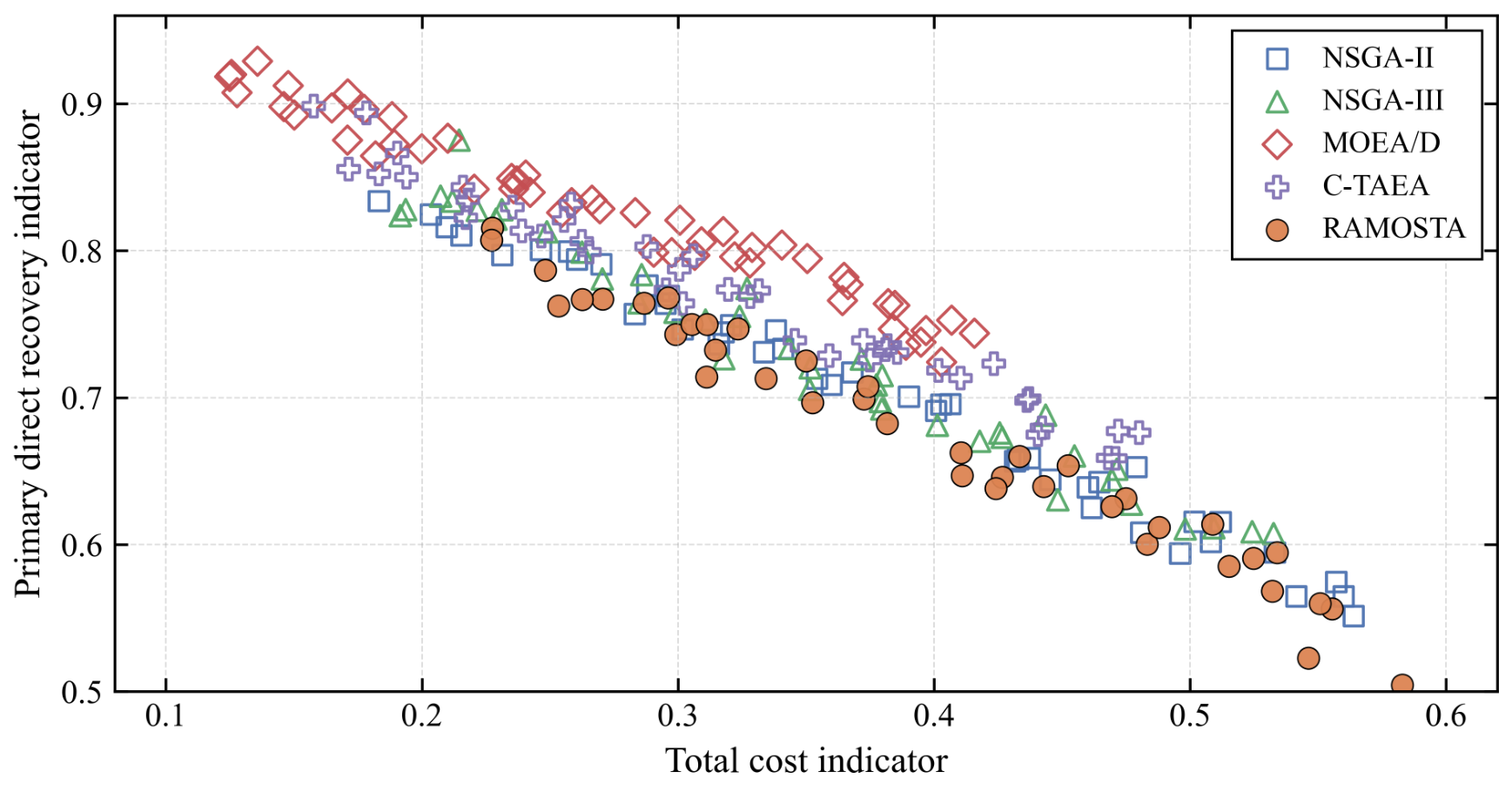
The Pareto fronts generated by the five compared algorithms, namely, NSGA-II, NSGA-III, MOEA/D, C-TAEA, and RAMOSTA, are presented in Figure 3. RAMOSTA produces a competitive and relatively well-distributed set of nondominated solutions compared with the four benchmark algorithms. Its solution set shows improved convergence toward the desirable trade-off region while maintaining coverage across the feasible search domain. These results indicate that RAMOSTA can balance exploration and exploitation under the process constraints and the uncertainty associated with surrogate evaluation.

For consistent metric calculation, all objective values were transformed into the same normalized three-objective minimization space before the HV and IGD calculations. Let $\mathcal{H}$ denote the feasible historical operating points that contain valid values for all three objectives after preprocessing and normalization. Let ${\mathcal{S}}_{\mathrm{high}}$ denote the feasible nondominated solutions obtained from an independent high-budget surrogate-assisted search conducted with the same objective definitions, normalization procedure, and constraint-handling rules. This independent search was not included in the 30 formal comparison runs.

The empirical reference Pareto set for IGD was constructed as

$${\mathcal{P}}_{\mathrm{ref}}=ND\left(\mathcal{H}\cup {\mathcal{S}}_{\mathrm{high}}\right),$$

(77)

where $ND(·)$ denotes nondominated filtering in the normalized three-objective minimization space. Before filtering, infeasible points and duplicate objective vectors were removed. The same ${\mathcal{P}}_{\mathrm{ref}}$ was used for all five algorithms and all independent runs.

For a nondominated solution set ${\mathcal{P}}_{a,r}$ generated by algorithm a in run r, the IGD is calculated as

$${IGD}_{a,r}={\displaystyle \frac{1}{|{\mathcal{P}}_{\mathrm{ref}}|}}\sum _{\mathbf{q}\in {\mathcal{P}}_{\mathrm{ref}}}\underset{\mathbf{p}\in {\mathcal{P}}_{a,r}}{min}{∥\mathbf{q}-\mathbf{p}∥}_2.$$

(78)

The historical operating points anchor the reference set to the feasible process regime represented by the confidential production data, whereas the independent high-budget search improves the coverage of trade-off regions that may be sparsely represented in the historical records. Therefore, ${\mathcal{P}}_{\mathrm{ref}}$ is interpreted as an empirical approximation of the data-supported Pareto front rather than as an exact global Pareto front.

For HV calculation, a single reference point was determined before comparing the algorithms. For each objective, the maximum value among all points in ${\mathcal{P}}_{\mathrm{ref}}$ was first calculated. The HV reference point was then defined as

$${\mathit{z}}_{\mathrm{HV}}^{\mathrm{ref}}={\mathit{z}}_{\max }+\gamma \left({\mathit{z}}_{\max }-{\mathit{z}}_{\min }+\epsilon \mathbf{1}\right),$$

(79)

where ${\mathit{z}}_{\max }$ and ${\mathit{z}}_{\min }$ are the component-wise maximum and minimum objective vectors in ${\mathcal{P}}_{\mathrm{ref}}$, $\gamma$ is a fixed positive margin coefficient, $\epsilon$ is a small numerical stabilizer, and $\mathbf{1}$ is a three-dimensional unit vector. The same normalized reference point was used for all five algorithms and all 30 independent runs. Because the problem was transformed into a minimization problem, the reference point was selected to be dominated by the objective vectors included in the HV calculation.

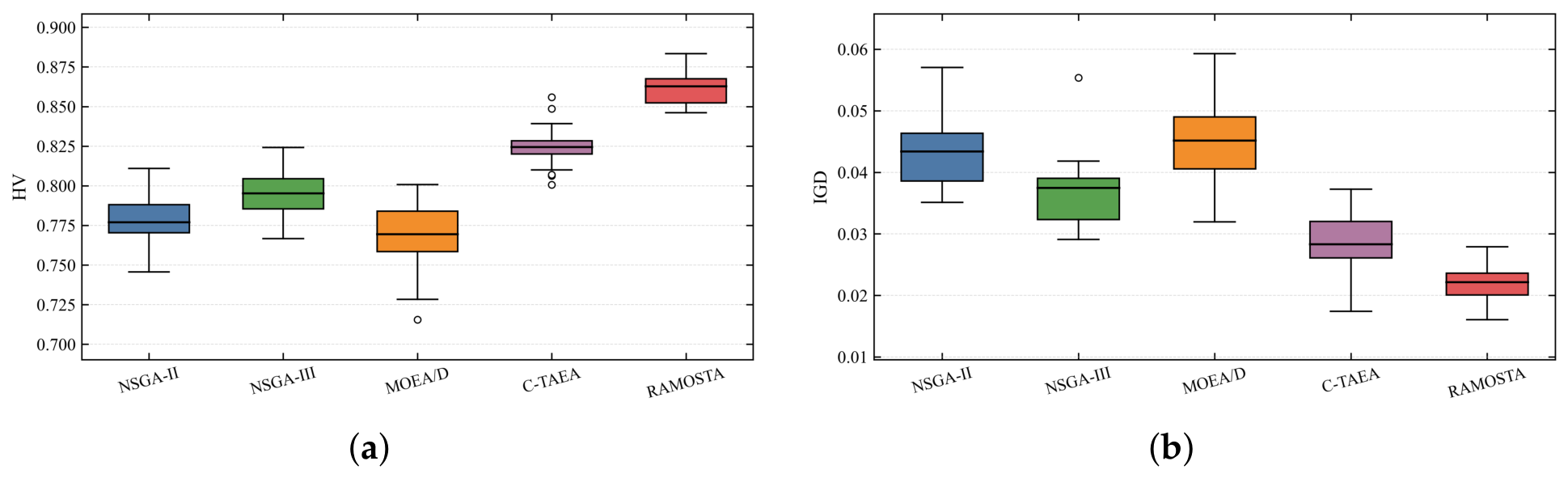
To quantify the optimization performance, Hypervolume (HV), Inverted Generational Distance (IGD), feasible ratio, and average runtime were used. HV measures the volume dominated by the obtained nondominated set with respect to the common reference point, and a larger value indicates better convergence and diversity. IGD measures the average distance from the empirical reference Pareto set to the obtained nondominated set, and a smaller value indicates better coverage of the reference set. The feasible ratio represents the proportion of evaluated solutions satisfying all specified operational and process constraints. Runtime represents the computational time required under the same implementation environment and evaluation protocol.

The statistical results over 30 independent runs are summarized in

Table 3. Performance metrics of NSGA-II, NSGA-III, MOEA/D, C-TAEA, and RAMOSTA over 30 independent runs.

Algorithm	HV ↑	IGD ↓	Feasible Ratio (%) ↑	Runtime (s) ↓
NSGA-II	$0.7814\pm 0.0187$	$0.0418\pm 0.0056$	$91.33\pm 4.72$	$31.84\pm 2.11$
NSGA-III	$0.7962\pm 0.0151$	$0.0365\pm 0.0049$	$93.67\pm 3.98$	$34.27\pm 2.46$
MOEA/D	$0.7689\pm 0.0204$	$0.0447\pm 0.0063$	$88.00\pm 5.21$	$28.93\pm 1.88$
C-TAEA	$0.8248\pm 0.0126$	$0.0294\pm 0.0037$	$97.00\pm 2.58$	$36.15\pm 2.73$
RAMOSTA	$0.8619\pm 0.0098$	$0.0217\pm 0.0029$	$100.00\pm 0.00$	$29.76\pm 1.94$

. RAMOSTA obtains the largest mean HV and the smallest mean IGD among the five compared algorithms, indicating a more favorable balance between convergence and solution-set distribution relative to the empirical reference front. RAMOSTA also achieves a feasible ratio of $100.00\%$ with zero reported standard deviation. This result should be interpreted in accordance with the feasibility definition and constraint-handling procedure adopted in this study: infeasible candidate solutions were identified through explicit process-constraint evaluation, and the implemented variable-bound projection, uncertainty-aware adaptive offset penalty, feasibility-prioritized selection, and archive-screening mechanisms prevented solutions retained for metric calculation from violating the specified constraints. Therefore, the reported $100.00\%$ feasible ratio indicates that all solutions included in the evaluated final archives satisfied the prescribed feasibility criteria; this does not imply that every intermediate candidate generated during the search was feasible. The absence of variation across the 30 runs further indicates that this feasibility-preserving procedure operated consistently under the tested experimental settings.

RAMOSTA does not necessarily achieve the shortest runtime because its computational procedure involves additional operations beyond objective-function and surrogate-model evaluations. In particular, each iteration requires uncertainty-indicator calculation, uncertainty-dependent offset adjustment, explicit constraint checking, adaptive penalty updating, feasibility-prioritized Pareto comparison, and candidate-archive maintenance. These additional operations increase the per-iteration computational overhead, even though they improve constraint handling and may contribute to the superior HV, IGD, and feasibility results. Consequently, runtime reflects a trade-off between computational efficiency and the additional calculations required for robust feasibility management, rather than serving as a direct measure of optimization quality.

From the computational perspective, RAMOSTA remains competitive in runtime. Although the adaptive offset mechanism requires additional uncertainty-related calculations, the mean runtime of RAMOSTA is lower than those of NSGA-II, NSGA-III, and C-TAEA, and is higher than that of MOEA/D in the reported experiments. Thus, the additional constraint-handling calculations do not result in a disproportionate computational burden in the present surrogate-assisted setting.

3.4. Representative Compromise Solution Analysis

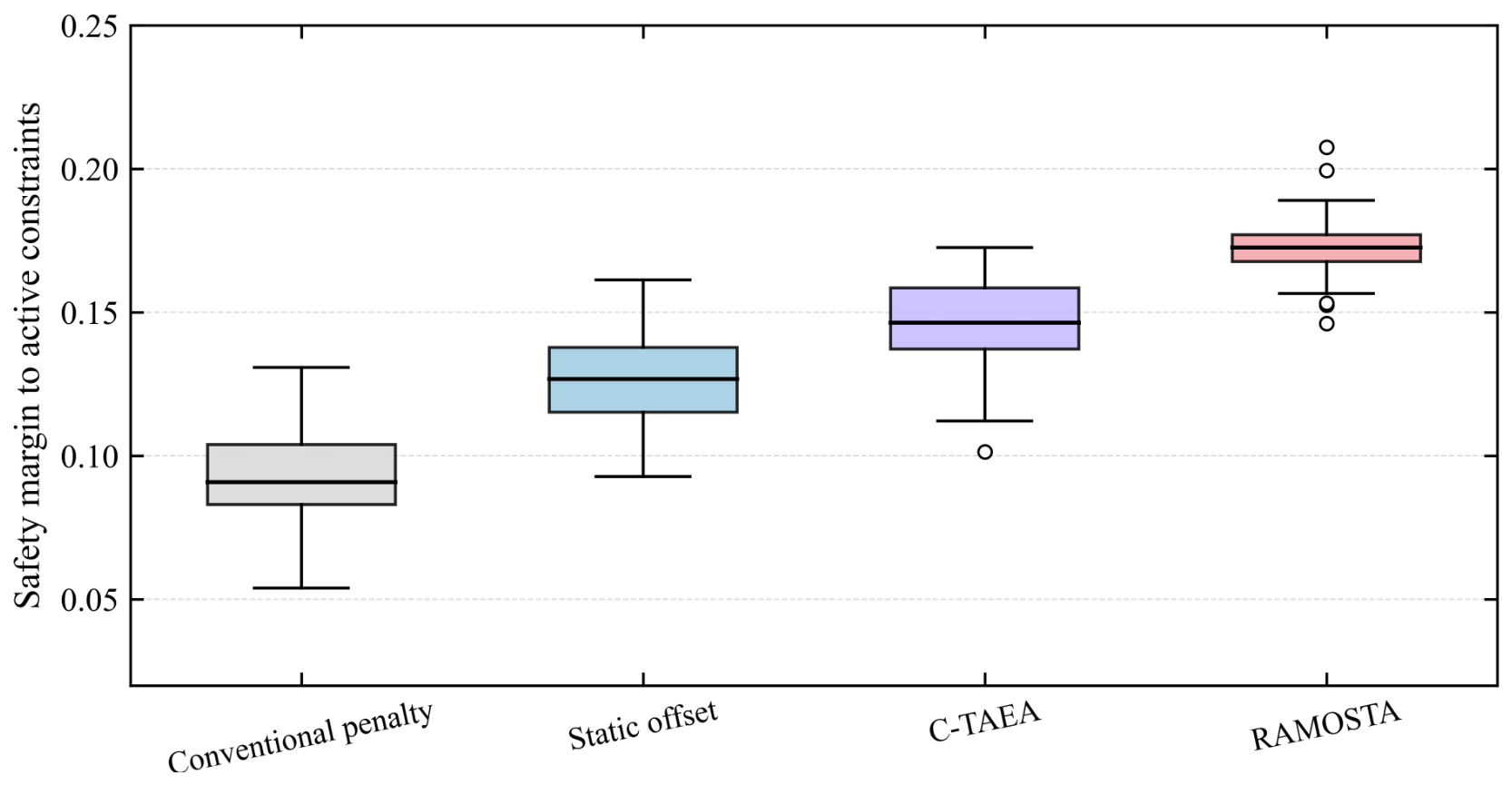
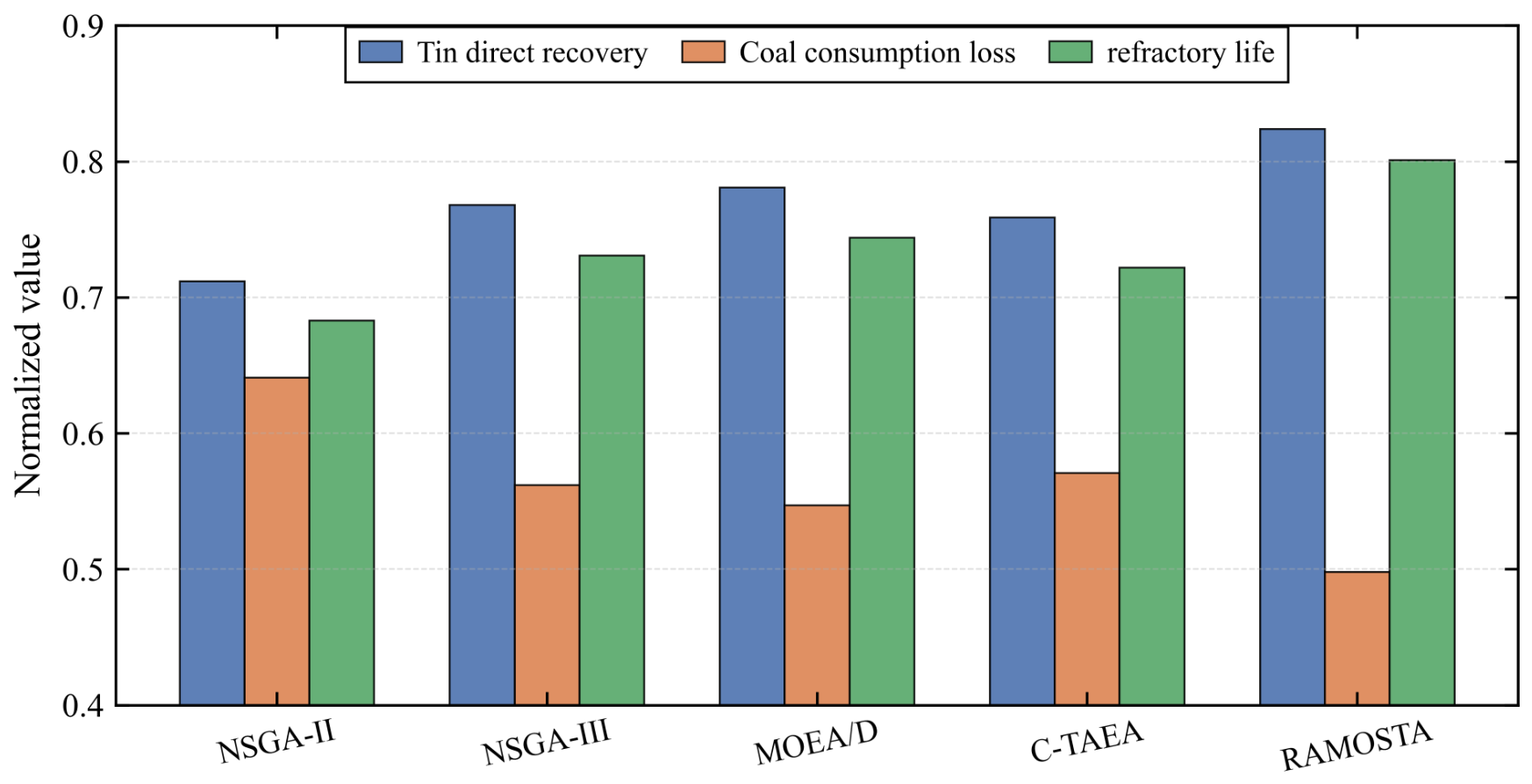
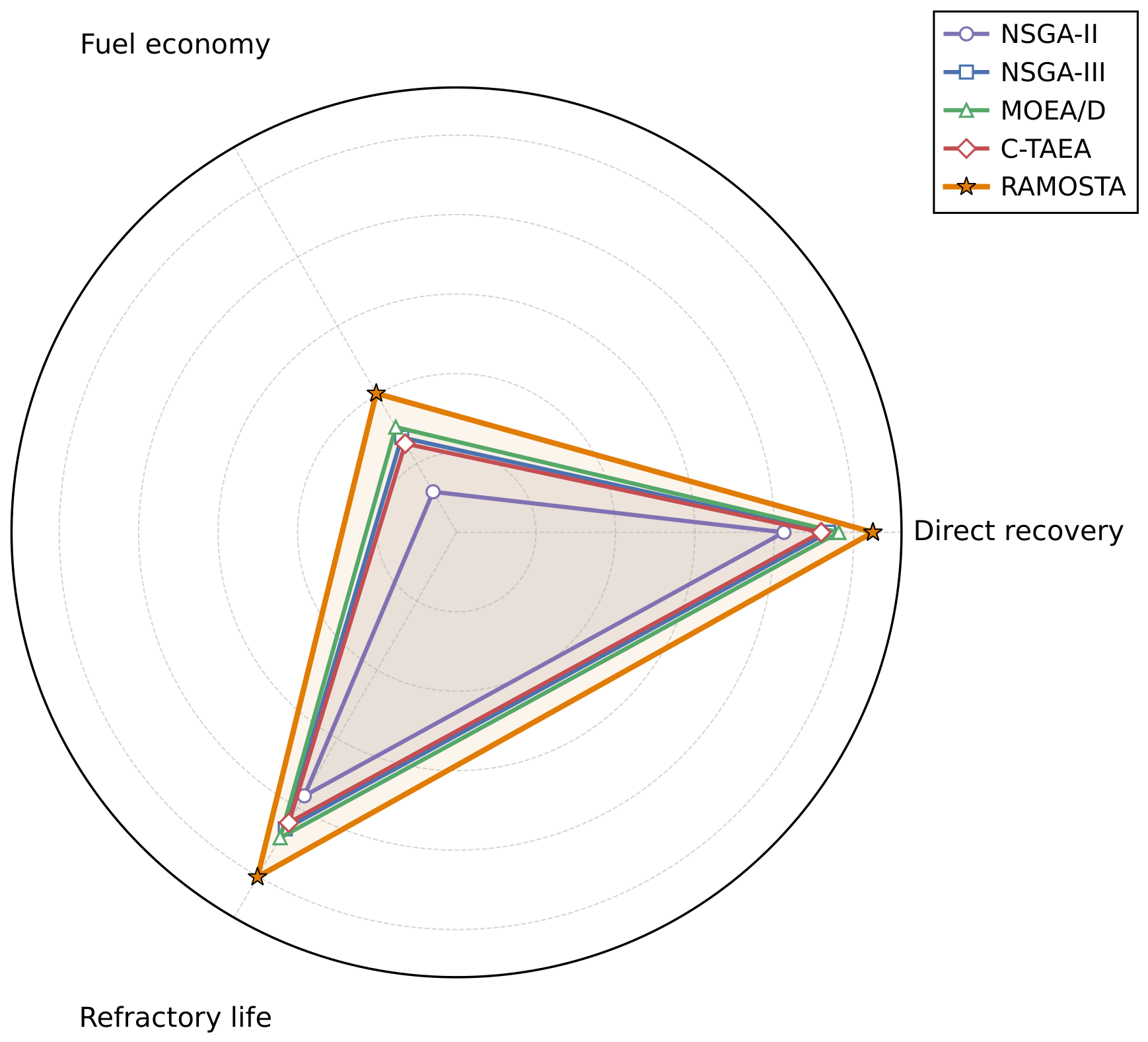
Although the Pareto front provides a set of candidate trade-off solutions, practical tin-smelting decision support requires the selection of one representative schedule. The decision maker therefore prefers a solution that provides a balanced combination of process performance, feasibility, and distance from active constraint boundaries rather than an extreme solution located near an uncertain boundary. Representative compromise schemes were selected from the nondominated sets generated by NSGA-II, NSGA-III, MOEA/D, C-TAEA, and RAMOSTA using the adaptive fusion decision mechanism.

The statistical comparison of the five algorithm-derived representative schemes is reported in

Table 4. Statistical comparison of representative compromise schemes generated by the five compared algorithms.

Scheme	Composite Utility ↑	Stability Margin ↑	Robustness Score ↑	Decision Consistency ↑
NSGA-II	$0.768\pm 0.032$	$0.127\pm 0.021$	$0.734\pm 0.030$	$0.786\pm 0.036$
NSGA-III	$0.781\pm 0.029$	$0.134\pm 0.019$	$0.748\pm 0.028$	$0.801\pm 0.033$
MOEA/D	$0.754\pm 0.035$	$0.121\pm 0.023$	$0.721\pm 0.034$	$0.774\pm 0.041$
C-TAEA	$0.809\pm 0.024$	$0.146\pm 0.017$	$0.781\pm 0.022$	$0.829\pm 0.028$
RAMOSTA	$0.853\pm 0.018$	$0.173\pm 0.014$	$0.826\pm 0.017$	$0.872\pm 0.021$

. The composite utility, stability margin, robustness score, and decision consistency are normalized decision-support indicators calculated according to the procedures defined in the experimental protocol, with larger values indicating preferable performance. RAMOSTA attains the largest mean value for all four indicators. This result is attributable to the combined effects of its search and solution-screening mechanisms rather than to the use of any algorithm-specific evaluation criterion. Specifically, the uncertainty-aware adaptive offset penalty and feasibility-prioritized selection reduce the likelihood that the final representative scheme is located near uncertain constraint boundaries, which is reflected in the stability-margin and robustness indicators. Meanwhile, the adaptive multiobjective search promotes solutions that maintain favorable trade-offs across the considered process objectives, contributing to higher composite utility. The archive-based retention and representative-scheme selection procedures further favor nondominated solutions with stable performance under the decision-support criteria, thereby improving decision consistency.

It should be noted that the four indicators are not fully independent, because they are calculated from the same normalized process responses, constraint information, and representative-scheme selection protocol. Therefore, RAMOSTA’s simultaneous superiority in these indicators should not be interpreted as four completely independent pieces of evidence. Rather, it indicates that, under the common evaluation framework used in this study, RAMOSTA more consistently identifies feasible and well-balanced representative schemes than the benchmark algorithms. All algorithms were evaluated using identical normalization rules, indicator definitions, and representative-scheme selection procedures; hence, the observed differences cannot be attributed to algorithm-specific post-processing or favorable metric definitions.

RAMOSTA obtains the largest mean values for all four indicators among the five compared algorithms. In particular, RAMOSTA achieves a composite utility of $0.853$, a stability margin of $0.173$, a robustness score of $0.826$, and a decision consistency of $0.872$ in the reported comparison. These results indicate that, within the offline evaluation environment, the RAMOSTA-derived compromise scheme provides a favorable balance between objective performance and constraint-related conservativeness.

The observed advantage is consistent with the coordinated use of the uncertainty-aware adaptive offset penalty and the adaptive weight fusion mechanism. The former discourages risky boundary-seeking solutions in uncertain regions, whereas the latter selects a compromise solution by combining preference information with objective information from the candidate set.

3.5. Statistical Significance and Robustness Verification

To examine the stability of the observed differences, the Wilcoxon rank-sum test was applied to the HV and IGD values obtained from the 30 independent runs of RAMOSTA and each benchmark algorithm. The significance level was set to $5\%$, and the results are summarized in

Table 5. Wilcoxon rank-sum test results of RAMOSTA against the four benchmark algorithms at the 5% significance level.

Compared Algorithm	p-Value on HV	Result	p-Value on IGD	Result
NSGA-II	$2.31\times {10}^{-5}$	+	$1.84\times {10}^{-5}$	+
NSGA-III	$4.92\times {10}^{-4}$	+	$3.17\times {10}^{-4}$	+
MOEA/D	$1.26\times {10}^{-5}$	+	$9.43\times {10}^{-6}$	+
C-TAEA	$1.71\times {10}^{-2}$	+	$2.36\times {10}^{-2}$	+

. All reported p-values are below the selected significance level. Therefore, under the stated 30-run comparison protocol, the HV and IGD distributions of RAMOSTA differ significantly from those of each benchmark algorithm.

This statistical result supports the repeatability of the observed differences in the present experimental setting. However, the test does not establish that every component of RAMOSTA independently causes the observed improvement. Component-level attribution requires separate ablation experiments.

Table 5 reports the Wilcoxon rank-sum test results, which statistically validate the superiority of RAMOSTA over the benchmark algorithms at the 5% significance level.

In addition to Pareto-front quality, robustness against constraint uncertainty was assessed through the normalized safety margin to active constraint boundaries, as shown in Figure 4, which compares the distributions of the normalized safety margin to the nearest active constraint boundary under four constraint-handling configurations. A larger value indicates that a candidate solution is farther from the closest active boundary and therefore retains a larger normalized constraint buffer. The conventional-penalty configuration has the lowest median safety margin and a relatively broad distribution, whereas the static-offset configuration shifts the distribution toward larger values. C-TAEA produces a further increase in the central tendency, although several lower-valued observations remain. RAMOSTA shows the highest median and an overall upward shift in the distribution, indicating that its retained candidate solutions are generally located farther from active constraint boundaries in the tested offline evaluation. The few outliers observed for RAMOSTA indicate that the solution set still contains candidates with different boundary distances and should not be interpreted as complete elimination of boundary-near solutions. Because this safety margin is a normalized decision-support indicator, the result should be understood as comparative evidence within the offline replay protocol rather than as a direct measurement of furnace safety or a causal proof of the independent contribution of the adaptive offset mechanism.

Figure 5 presents the boxplots of HV and IGD over the 30 independent runs. RAMOSTA shows a higher median HV, a lower median IGD, and a narrower interquartile range than the benchmark algorithms in the reported results. These distributions indicate more consistent performance across independent runs in the present experimental setting.

3.6. Adaptive Offset Penalty Analysis

To examine the contribution of the uncertainty-aware adaptive offset penalty, an ablation comparison was conducted under the same data representation, surrogate models, objective definitions, population settings, evaluation budget, and termination conditions. The complete RAMOSTA configuration was compared with a variant without the adaptive offset penalty. In the ablated variant, the same constraint-handling framework was retained, but the uncertainty-dependent offset term was removed from the penalty calculation. Thus, the comparison isolates the effect of the adaptive offset mechanism without changing the other optimization components.

The comparison used HV, IGD, feasible ratio, and normalized safety margin. HV and IGD were calculated using the common reference point and empirical reference Pareto set defined in Section 3.3. The feasible ratio was calculated from the proportion of evaluated solutions satisfying all specified constraints. The normalized safety margin was calculated as the minimum normalized distance from a feasible candidate to the active constraint boundaries. A larger safety margin indicates a greater distance from the nearest active boundary.

The results are reported in

Table 6. Ablation comparison of the adaptive offset penalty.

Configuration	HV ↑	IGD ↓	Feasible ratio (%) ↑	Safety margin ↑
Without adaptive offset	$0.823$	$0.031$	$95.40$	$0.142$
Complete	$0.862$	$0.022$	$100.00$	$0.173$

. The complete RAMOSTA configuration is expected to provide better constraint-related reliability than the variant without the adaptive offset term, particularly when candidate solutions are located near uncertain boundary regions. If the complete configuration produces a larger feasible ratio and safety margin together with improved HV or IGD, this would support the intended role of the adaptive offset penalty. However, the results should be interpreted as evidence for the tested configuration and should not be used to attribute all performance differences solely to this component without considering the experimental variability.

The ablation comparison also provides a direct check of whether the uncertainty indicator affects the optimization behavior in the intended direction. A lower safety margin or a higher infeasible proportion in the variant without the offset term would indicate that removing the uncertainty-dependent adjustment makes the search more likely to approach risky constraint regions. The analysis therefore complements the overall algorithm comparison by examining the specific constraint-handling mechanism of RAMOSTA.

3.7. Industrial Decision Support Analysis

To assess the decision-support value of the proposed framework, the nondominated solutions generated by NSGA-II, NSGA-III, MOEA/D, C-TAEA, and RAMOSTA were further processed using the defined compromise-solution selection procedure. Given the production conditions and operational requirements represented in the confidential offline data, the procedure first generates candidate nondominated solutions and then selects a final recommendation according to the adaptive weight fusion mechanism.

In the reported offline replay, the RAMOSTA-derived strategy shows improved decision consistency and lower fluctuation according to the defined normalized indicators. These results suggest that the selected compromise solutions have decision-support potential under the evaluated historical process conditions. They do not constitute prospective evidence of closed-loop production improvement.

Figure 6 compares the average normalized benefit-oriented performance of the five algorithms over the replay horizon. RAMOSTA achieves the highest normalized direct tin recovery and refractory-life scores, while obtaining the lowest normalized coal-consumption loss among the compared methods in the reported offline evaluation. The coal-consumption-related loss and refractory-life response are transformed according to their optimization directions so that larger normalized scores represent preferable performance.

Among the benchmark algorithms, NSGA-II, NSGA-III, MOEA/D, and C-TAEA also show optimization capability. The similar average normalized performance of NSGA-III, MOEA/D, and C-TAEA indicates that their representative schemes achieved comparable aggregated results under the common offline replay and normalization procedure. Because the plotted values are averaged normalized indicators, relatively small differences in individual objectives or constraint margins may not be visually distinguishable in the bar chart. Their relative performance should therefore be interpreted together with the Pareto-quality, feasibility, and statistical results. RAMOSTA provides the best reported balance among direct tin recovery, coal-consumption loss, and refractory life in the present offline replay.

For a more intuitive comparison, Figure 7 presents a radar chart of the three normalized aggregated indicators. The coal-consumption-related loss is converted into a fuel-economy score for visualization, and the refractory-life response is transformed according to its optimization direction. The larger enclosed area of RAMOSTA indicates a more favorable balance among the three normalized indicators in the reported offline comparison.

Figure 7 presents the normalized benefit-oriented scores of direct tin recovery, fuel economy, and refractory-life performance. The larger enclosed area of RAMOSTA is associated with its relatively high direct-recovery and refractory-life scores, while its fuel-economy score remains competitive with those of the other methods. Because the area is jointly determined by the three normalized axes and their interactions, it cannot be attributed to any single objective. The radar chart therefore illustrates the overall balance of the three indicators in the offline replay rather than proving that one specific indicator is solely responsible for the observed difference.

To examine the stability of the final recommendation, a decision-weight sensitivity analysis was conducted. The baseline decision weights were perturbed within a prescribed relative range while preserving the normalization procedure and the candidate nondominated sets. For each perturbed weight setting, the adaptive fusion mechanism was reapplied to the same candidate solutions, and the resulting representative scheme was recorded. The analysis focused on the selected-scheme consistency, composite utility, and normalized refractory-life score.

The sensitivity-analysis results are summarized in

Table 7. Sensitivity of the RAMOSTA-derived representative scheme to decision-weight perturbations.

Weight Setting	Scheme Consistency (%) ↑	Composite Utility ↑	Refractory-Life Score ↑
Baseline weights	$100.0\pm 0.0$	$0.853\pm 0.000$	$0.826\pm 0.000$
Fluctuation $\pm 5\%$	$96.7\pm 1.2$	$0.849\pm 0.004$	$0.821\pm 0.003$
Fluctuation $\pm 10\%$	$93.3\pm 2.1$	$0.842\pm 0.007$	$0.815\pm 0.006$
Fluctuation $\pm 20\%$	$86.7\pm 3.5$	$0.827\pm 0.012$	$0.801\pm 0.010$

. All weight settings were evaluated using the same RAMOSTA candidate set and identical offline replay conditions. Thus, the observed changes in the selected representative scheme arise solely from changes in the decision-preference weights, rather than from stochastic variation in the optimization process or differences in the candidate solutions.

As the weight perturbation range increases, the variation in the decision-support scores generally becomes larger and the selected-scheme consistency correspondingly decreases. This behavior is expected because the final recommendation is determined by a weighted aggregation of multiple normalized criteria. Under small perturbations, the relative ranking of the leading candidate schemes is usually preserved, particularly when the baseline selected scheme has a sufficient score advantage over competing schemes. Consequently, the same scheme, or schemes with very similar performance, is repeatedly selected. When the perturbation magnitude increases, the contribution of individual criteria to the aggregated score changes more substantially. Candidate schemes with different strengths, such as higher utility but lower robustness, or greater stability but lower composite utility, may then exchange their ranking positions. This produces larger fluctuations in the selected-scheme statistics and reduces the frequency with which the baseline scheme remains the final recommendation.

The decrease in consistency should therefore not be interpreted as instability in the RAMOSTA optimization procedure. Instead, it reflects the expected sensitivity of a multi-criterion decision result when decision preferences are deliberately varied over a wider range. In particular, a more pronounced reduction in consistency may occur when several candidate schemes have similar baseline aggregate scores, because even moderate changes in criterion weights can alter their ranking. Conversely, the consistency values obtained under small and moderate perturbations quantify the robustness of the recommendation to plausible preference uncertainty. Overall, Table 7 indicates the range over which the recommended scheme remains stable and identifies the point at which changes in decision preference become sufficiently large to favor alternative, yet still competitive, feasible schemes.

The sensitivity analysis should be interpreted as a robustness check for the decision layer rather than as a validation of the optimization layer. If moderate weight perturbations preserve the selected scheme or produce only small changes in the composite utility and refractory-life score, the final recommendation can be considered stable under the tested preference variations. If the selected scheme changes frequently, the decision layer should be reported as preference-sensitive, and the final recommendation should not be described as uniquely determined.

In summary, the offline replay results show differences in Pareto-front quality, feasibility, and compromise-solution performance among NSGA-II, NSGA-III, MOEA/D, C-TAEA, and RAMOSTA under the tested confidential evaluation protocol. The decision-weight sensitivity analysis further provides a check of the stability of the RAMOSTA-derived recommendation under moderate preference changes. These results should be interpreted within the stated dataset, surrogate-model assumptions, and offline evaluation conditions.

4. Discussion on Optimization Effectiveness, Industrial Relevance, and Future Limitations

The comparative results show that RAMOSTA achieved a favorable balance between Pareto-front quality and constraint satisfaction under the adopted evaluation protocol. The reported HV, IGD, and feasible-ratio results indicate improvements in convergence, solution coverage, and feasibility relative to the benchmark methods, while the Wilcoxon-test results suggest that these differences were generally repeatable across the 30 independent runs. The constraint-margin analysis further shows that the retained solutions were, on average, farther from the active constraint boundaries than those obtained with the alternative constraint-handling configurations. This result is consistent with the uncertainty-dependent offset, which discourages candidates located close to boundaries in regions with larger bootstrap-model dispersion. These findings are based on a data-supported reference set and offline surrogate-assisted evaluations; therefore, they indicate comparative performance under the stated protocol rather than optimality relative to an exact global Pareto front.

The final compromise-scheme analysis indicates that the selected RAMOSTA solution provided a favorable joint balance among direct tin recovery, energy consumption, constraint margin, and the normalized refractory-degradation indicator. The composite utility, stability margin, robustness score, and decision consistency are calculated under a common normalization and selection procedure and should not be interpreted as fully independent performance measures. The hybrid-weight decision layer combines expert preference with objective discrimination derived from the Pareto archive, with the fusion coefficient determined from the cosine similarity between the subjective and objective weight vectors. The offline replay comparison also suggests favorable relative performance under the historical conditions represented in the dataset. However, $Q_{\mathrm{ref}}$ is a normalized process indicator for the relative degradation level of the magnesia–chrome refractory lining, rather than a direct measurement of thickness loss or refractory campaign life.

Several limitations remain. The reliability of the surrogate-assisted optimization depends on the quality and coverage of the historical production data, and prediction accuracy may decrease in rarely observed operating regions or after substantial changes in feed composition, equipment condition, or operating policy. The bootstrap standard deviation is used as an empirical model-disagreement measure for conservative constraint handling; it is not a calibrated confidence interval or a formal probability bound. In addition, the refractory-related objective would benefit from direct refractory-degradation or campaign-life observations. Future work should therefore consider broader operating-data coverage, uncertainty calibration, direct refractory-condition measurements, and controlled ablation studies to quantify the individual contributions of the state-transition model, offset penalty, surrogate updating strategy, and hybrid-weight decision layer.

5. Conclusions

This study developed a RAMOSTA-based framework for offline, surrogate-assisted dynamic multiobjective optimization of top-blowing furnace operation in tin smelting. The framework combines 11-dimensional RBFN response approximation, dynamic state-transition search, bootstrap-based constraint tightening, and hybrid-weight TOPSIS selection to address nonlinear responses, conflicting objectives, limited historical labels, expensive direct evaluations, and strict feasibility requirements. Under the confidential chronological-data and offline replay protocol, RAMOSTA achieved a mean HV of $0.8619\pm 0.0098$, a mean IGD of $0.0217\pm 0.0029$, and the highest feasible ratio among NSGA-II, NSGA-III, MOEA/D, and C-TAEA. The constraint-margin analysis also indicated that the obtained solutions generally maintained larger normalized margins than the alternative configurations. For the final compromise-scheme selection, the composite utility was calculated together with fluctuation indicators under the common normalization procedure; therefore, larger operating fluctuations reduce the composite utility when fluctuation is treated as a cost-type criterion. The refractory-related term in the decision analysis refers specifically to the normalized magnesia–chrome refractory-degradation indicator $Q_{\mathrm{ref}}$, rather than to a direct measurement of refractory thickness loss or campaign life. The subjective and data-derived weights were combined using the cosine-similarity-based fusion rule, and the candidate with the largest TOPSIS relative-closeness coefficient was selected as the representative operating schedule.