Identification of Combined Isotropic–Kinematic Hardening Parameters from Reverse Bending Tests Using Recurrent Neural Networks

Abstract

Accurate identification of constitutive parameters is essential for reliable finite element simulations of sheet metal forming processes. Conventional inverse identification techniques, such as Finite Element Model Updating (FEMU), generally require iterative optimization procedures involving numerous finite element simulations, resulting in high computational cost. This work proposes a machine learning framework based on a bidirectional Long Short-Term Memory (Bi-LSTM) neural network for the identification of combined isotropic–kinematic hardening parameters from a custom-designed reverse bending test. A synthetic dataset comprising 5000 finite element simulations was generated by systematically varying the parameters of the Swift isotropic hardening law and the Armstrong–Frederick kinematic hardening law using Sobol sampling. The resulting force–displacement histories were used to train the Bi-LSTM network to predict five constitutive parameters (K, ${\sigma }_0$, n, C, and $\gamma$) directly from force–displacement responses. To improve the physical admissibility of the predictions, a physically constrained loss function was introduced by penalizing negative values of the kinematic hardening parameters during training. The proposed model achieved coefficients of determination, $R^2$ above 0.98 for the isotropic and kinematic hardening parameters while reducing the number of physically inadmissible predictions from approximately 30 to a single case. Experimental validation was performed on DP500 and DP780 advanced high-strength steels, where finite element simulations using the Bi-LSTM predicted parameters reproduced the experimentally measured springback angles with good agreement. The proposed methodology provides near-instantaneous constitutive parameter identification after training, eliminating the need for computationally expensive iterative optimization while maintaining high predictive accuracy and physical consistency.

1. Introduction

Material constitutive models play a fundamental role in materials science and manufacturing processes by providing a mathematical description of material behavior under different loading conditions. In computational mechanics, they are a key component of numerical simulations of manufacturing processes, particularly finite element (FE) analysis of forming operations, where they govern the predicted mechanical response of the material. For sheet metal materials, constitutive modeling approaches can generally be divided into two main categories: (i) crystallographic texture-based models and (ii) phenomenological models. Crystallographic texture-based models rely on crystal plasticity theory, describing deformation through crystallographic slip systems and incorporating texture information to capture anisotropic behavior [1,2]. Although they provide a physically based representation of material response, their high computational cost limits their application in large-scale industrial forming simulations [3].

Phenomenological models, in contrast, describe the macroscopic mechanical response through mathematical formulations calibrated against experimental observations. Although some phenomenological formulations incorporate concepts motivated by crystallographic mechanisms, their constitutive parameters are generally identified by minimizing the difference between numerical predictions and experimental measurements [4]. In this context, the constitutive models chosen to represent the behavior of the material have a significant impact on the accuracy of sheet metal forming simulations by FEA. This behavior normally includes four independent but interconnected phenomena [5]: (a) the elastic behavior and its influence on springback [6]; (b) the yield criterion [7,8]; (c) the forming limits and (d) the hardening model [9]. Regarding the hardening laws, the major developments include the study of kinematic and distortional hardening [10] through the description of the tension–compression stress differential (SD), the Bauschinger effect, work-hardening stagnation, permanent softening and cross-loading effects. These mechanisms are particularly important for advanced materials such as Advanced High-Strength Steels (AHSS), which require accurate representation to predict material behavior under complex loading path changes in sheet metal forming applications [11]. Recent advances in this topic have led to the increased complexity of modern constitutive models with additional empirical parameters, making the calibration procedure more difficult and time-consuming, particularly when multiple experimental tests are required [12].

To address the challenges associated with parameter identification in phenomenological models, several inverse identification strategies have been proposed. These approaches combine experimental measurements with numerical simulations to characterize material behavior under different stress and strain states. Common inverse identification techniques include Finite Element Model Updating (FEMU) [13], the Constitutive Equation Gap Method (CEGM) [14], the Virtual Fields Method (VFM) [15], and the Equilibrium Gap Method (EGM) [16]. These approaches are commonly coupled with optimization algorithms, which may be gradient-based or derivative-free. However, their performance strongly depends on the characteristics of the identification problem. Gradient-based methods can be sensitive to the initial parameter estimation, while derivative-free methods, although less dependent on initial conditions, may still converge towards local optima in highly nonlinear problems. Consequently, global optimization strategies, such as genetic algorithms, have been investigated to improve solution robustness, although at the expense of increased computational costs [17].

In response to these computational limitations, machine learning (ML) has emerged as a powerful tool for parameter identification in constitutive modeling. Rather than relying on iterative optimization, ML-based approaches enable the direct prediction of constitutive parameters from experimental observations through a trained surrogate model. These approaches generally follow a two-stage workflow. First, a synthetic dataset is generated using finite element simulations covering different geometries, loading conditions, and constitutive parameter combinations. The resulting mechanical responses are then used to train an ML model to learn the inverse mapping between measurable quantities (e.g., displacement or strain fields) and the corresponding material parameters. Once trained, the ML model enables almost instantaneous parameter identification from experimental measurements, reducing the computational cost associated with conventional inverse identification procedures [18,19,20,21]. Several authors have demonstrated the effectiveness of artificial neural network (ANN)-based approaches for parameter identification. Huber et al. [22] developed a feedforward neural network (FNN) to identify parameters of a finite deformation viscoplasticity model, achieving good agreement with experimental data even under complex loading histories. Ktari et al. [23] applied FNNs to identify anisotropic parameters based on experimental tests. Bouchard et al. [24] highlighted the integration of inverse identification procedures with full-field measurement techniques, reinforcing the effectiveness of ANN-based strategies in experimental settings. Beyond standard ANN-based approaches, hybrid methods coupling neural networks with genetic algorithms have also been developed. Aguir et al. [18] focused on calibrating the Karafillis–Boyce yield surface combined with a Voce hardening law, where ANNs trained on finite element data approximated mechanical responses for given parameter sets, and a genetic algorithm explored the parameter space iteratively. Yao et al. [25] extended this concept to viscoplastic-damage models, using ANNs to generate informed initial populations for optimization loops, achieving accurate parameter identification under diverse loading conditions.

In addition to ANN-based models, alternative machine learning models have also been explored. Huang et al. [26] applied Gaussian Process Regression (GPR), a non-parametric Bayesian approach for the inverse identification of Swift hardening and Lemaitre damage model parameters, based on tensile test simulations of AA2017-T4 aluminum. The surrogate predictions were then integrated into finite element analyses and successfully validated against experimental results, highlighting the potential of probabilistic surrogate models in constitutive parameter calibration. Bastos et al. [27] applied the XGBoost algorithm for the identification of elastoplastic constitutive parameters, using synthetic full-field data generated by finite element simulations of heterogeneous dogbone tests. Their study showed that gradient-boosted trees could achieve highly accurate predictions with relatively small training datasets and that dimensionality reduction techniques such as Principal Component Analysis (PCA) improved computational efficiency without compromising accuracy. More recent studies have further expanded the use of machine learning for sheet metal constitutive parameter identification. Marques et al. [28] compared several machine learning algorithms using datasets based on uniaxial and biaxial tensile responses. Their results showed that GPR achieved the best predictive performance among the investigated methods, while SHAP analysis was used to assess input-feature relevance. Tariq and Deliktaş [29] proposed a machine-learning-aided inverse identification framework combining finite element analysis, optimization, and machine learning techniques. Their results demonstrated the potential of machine learning to reduce the computational cost associated with conventional iterative inverse identification. A critical challenge in deploying neural networks for parameter identification is ensuring robustness of the training dataset. Mitreiro et al. [30] addressed mesh dependency effects in synthetic dataset generation, demonstrating that finite element mesh resolution can significantly impact model predictions and generalization to experimental data. This work highlights the importance of careful dataset construction when transitioning from laboratory to industrial scales, and underscores the necessity of synthetic-to-real validation.

An important advancement was introduced by Morand and Helm [31], who addressed the issue of non-uniqueness in parameter identification. For certain constitutive models, different parameter combinations may produce nearly identical macroscopic responses, making the inverse problem inherently ambiguous. In such cases, conventional single ANN surrogate models tend to learn an average representation of the possible solutions, leading to reduced prediction accuracy. To overcome this limitation, the authors proposed a mixture of experts approach, in which multiple ANNs are trained in parallel and dynamically combined through a gating network. The proposed framework outperformed conventional single-network models in both numerical benchmarks and experimental validation on AA6014 aluminum, DC04, and DP600 steels, demonstrating improved robustness and accuracy for non-unique parameter identification problems.

More recently, deep learning architectures have been explored to improve the robustness of inverse parameter identification when dealing with noisy or high-dimensional experimental data. In particular, convolutional neural networks (CNNs) and recurrent neural networks (RNNs) have shown promising results. Guo et al. [32] proposed a hybrid CNN–LSTM framework in which convolutional layers extract relevant features and mitigate experimental noise, while long short-term memory (LSTM) layers capture the sequential nature of loading histories. Trained on finite element-generated data, the model accurately identified five elastoplastic parameters and demonstrated prediction accuracy comparable to FEMU-based approaches while providing near-instantaneous inference. Experimental validation on AA6061 aluminum further confirmed its effectiveness.

Recurrent architectures have received comparatively little attention in inverse parameter identification, despite their ability to capture sequential dependencies inherent to history-dependent material behavior. Cruz et al. [33] applied LSTMs to identify the parameters of the Swift hardening law from three-point bending experiments, demonstrating the feasibility of recurrent neural networks for sequence-based constitutive parameter identification. In contrast, recurrent architectures have been more extensively explored in fully data-driven constitutive modeling, where the stress–strain evolution is learned directly from loading histories without assuming an explicit constitutive formulation. By replacing conventional constitutive equations with trained machine learning models, these approaches can be readily integrated into finite element simulations, substantially reducing simulation times while maintaining predictive accuracy [34,35,36,37,38,39].

Despite these advances, most machine learning methodologies have focused on the identification of constitutive parameters associated with isotropic hardening. Although machine learning has previously been applied to identify the parameters of kinematic hardening models [40,41], its application to sheet metal materials remains very limited. This is particularly important because sheet metal forming processes frequently involve complex loading paths with stress reversals, where an accurate description of the Bauschinger effect requires constitutive models incorporating kinematic hardening. Consequently, the inverse identification of these models is considerably more challenging than that of isotropic hardening, since the material response depends on the entire deformation history rather than solely on the current deformation state.

To address this limitation, the present work extends the machine learning framework developed by Cruz et al. [33] to the inverse identification of combined isotropic–kinematic hardening parameters from sheet metal reverse bending responses. A novel reverse bending test is proposed to induce strain-path reversals and activate the Bauschinger effect, thereby providing rich information for calibrating kinematic hardening models. The proposed methodology combines this experimental configuration with a bidirectional long short-term memory (Bi-LSTM) network to identify constitutive parameters directly from measured force–displacement histories. In addition, a physically constrained loss function is introduced to promote physically admissible predictions of the constitutive parameters during network training. Finally, the proposed framework is validated using both numerical simulations and experimental reverse bending tests.

This document is organized as follows. Section 2 presents the constitutive model, the reference constitutive parameters, and the proposed reverse bending test. Section 3 describes the machine learning framework, including the generation of the synthetic dataset, the Bi-LSTM architecture, and the training strategy adopted for constitutive parameter identification. Section 4 presents the numerical and experimental validation of the proposed methodology, including the assessment of the physically constrained loss function and the sensitivity of the predictions to force-measurement noise. Finally, Section 5 summarizes the main findings and outlines directions for future work.

2. Materials and Methods

2.1. Constitutive Model

The constitutive model adopted in this work combines isotropic and kinematic hardening formulations. The combination of these hardening mechanisms enables the yield surface to undergo both isotropic expansion and kinematic translation during plastic deformation. The isotropic hardening component is described by the Swift law [42]:

$${\sigma }_y=K{({\epsilon }_0+{\overline{\epsilon }}_p)}^n,$$

(1)

where K is the strength coefficient, ${\epsilon }_0$ is the offset strain, n is the strain-hardening exponent, and ${\overline{\epsilon }}_p$ is the equivalent plastic strain. The initial yield stress, ${\sigma }_0$, is obtained from the Swift law by setting ${\overline{\epsilon }}_p=0$:

$${\sigma }_0=K{\epsilon }_0^n.$$

(2)

The kinematic hardening component accounts for the translation of the yield surface in stress space. This translation is described by the backstress tensor, $\mathit{\alpha }$, allowing the model to capture the Bauschinger effect observed during load reversals. The nonlinear evolution of the backstress is described using the Armstrong–Frederick model [43], which extends the classical Prager linear kinematic hardening law [44] by introducing a dynamic recovery term. This formulation allows the backstress to progressively saturate with increasing plastic deformation. The evolution equation is expressed as:

$$\dot{\mathit{\alpha }}={\displaystyle \frac{2}{3}}C{\dot{\mathit{\epsilon }}}_p-\gamma \mathit{\alpha }{\dot{\overline{\epsilon }}}_p,$$

(3)

where C is the initial kinematic hardening modulus, $\gamma$ is the dynamic recovery parameter that controls the saturation rate of the backstress, ${\dot{\mathit{\epsilon }}}_p$ is the plastic strain rate tensor, and ${\dot{\overline{\epsilon }}}_p$ is the equivalent plastic strain rate.

The constitutive model is therefore defined by five material parameters: K, ${\sigma }_0$, and n, which describe the isotropic hardening behavior, and C and $\gamma$, which govern the kinematic hardening response. Accordingly, the constitutive parameter identification problem addressed in this work consists of estimating these five material parameters from experimental observations using the proposed machine learning framework.

2.2. Materials and Reference Constitutive Parameters

The methodology proposed in this work is intended for sheet steels commonly used in metal forming applications, ranging from conventional mild steels to advanced high-strength steels (AHSS). To validate the proposed ML framework, two representative dual-phase steels, DP500 and DP780, with a nominal sheet thickness of 0.8 mm, were selected as case studies. Their chemical compositions are listed in

Table 1. Chemical composition of the dual-phase steels (DP500, DP780).

Element [%]	C	Si	Mn	P	S	Cr	Ni	V	Cu	Al	Nb	B	N
DP500	0.079	0.31	0.65	0.003	0.003	0.03	0.03	0.01	0.01	0.038	0.0	0.0003	0.003
DP780	0.138	0.20	1.52	0.011	0.002	0.03	0.03	0.02	0.01	0.038	0.014	0.0002	0.003

.

The reference constitutive parameters for these materials were obtained from previously published experimental studies. The parameters of the Swift isotropic hardening model (IH) were taken from the experimental characterization reported in [45] and were identified from uniaxial tensile tests, performed in accordance with [46]. The parameters of the combined isotropic–kinematic hardening (IKH) model were identified from the cyclic tension–compression experiments on miniaturized specimens reported by Cruz et al. [47]. The experimental methodology, including the specimen geometry and testing procedure, is described in detail in [47]. The experimental stress–strain curves obtained from these tests were used in an inverse finite element identification procedure based on a genetic algorithm (GA) to identify the IKH constitutive parameters.

Table 2. Identified parameters of the Swift isotropic hardening (IH) model for the DP500 and DP780 dual-phase steels obtained from uniaxial tensile tests.

Isotropic Hardening (IH)
Material	$\mathit{K}$ [MPa]	${\mathit{\epsilon }}_{\mathbf{0}}$	$\mathit{n}$
DP500	865.32	0.0026	0.1530
DP780	1253.72	0.0001	0.1431

and

Table 3. Identified isotropic–kinematic hardening (IKH) parameters for the DP500 and DP780 dual-phase steels obtained from tension–compression tests.

Combined Isotropic–Kinematic Hardening (IKH)
Material	$\mathit{K}$ [MPa]	${\mathit{\epsilon }}_{\mathbf{0}}$	$\mathit{n}$	$\mathit{C}$ [MPa]	$\mathit{\gamma }$
DP500	632.6	0.082	0.334	27,710	124.2
DP780	651.8	0.054	0.191	38,850	88.3

summarize the identified material parameters for the DP500 and DP780 steels using the Swift isotropic hardening law and the combined isotropic–kinematic hardening model, respectively.

It should be noted that the parameters reported in Table 2 and Table 3 were obtained from different calibration procedures and should therefore not be directly compared on a parameter-by-parameter basis. In particular, the identified value of ${\epsilon }_0$ depends on the corresponding K and n values, since the initial yield stress is determined according to Equation (2).

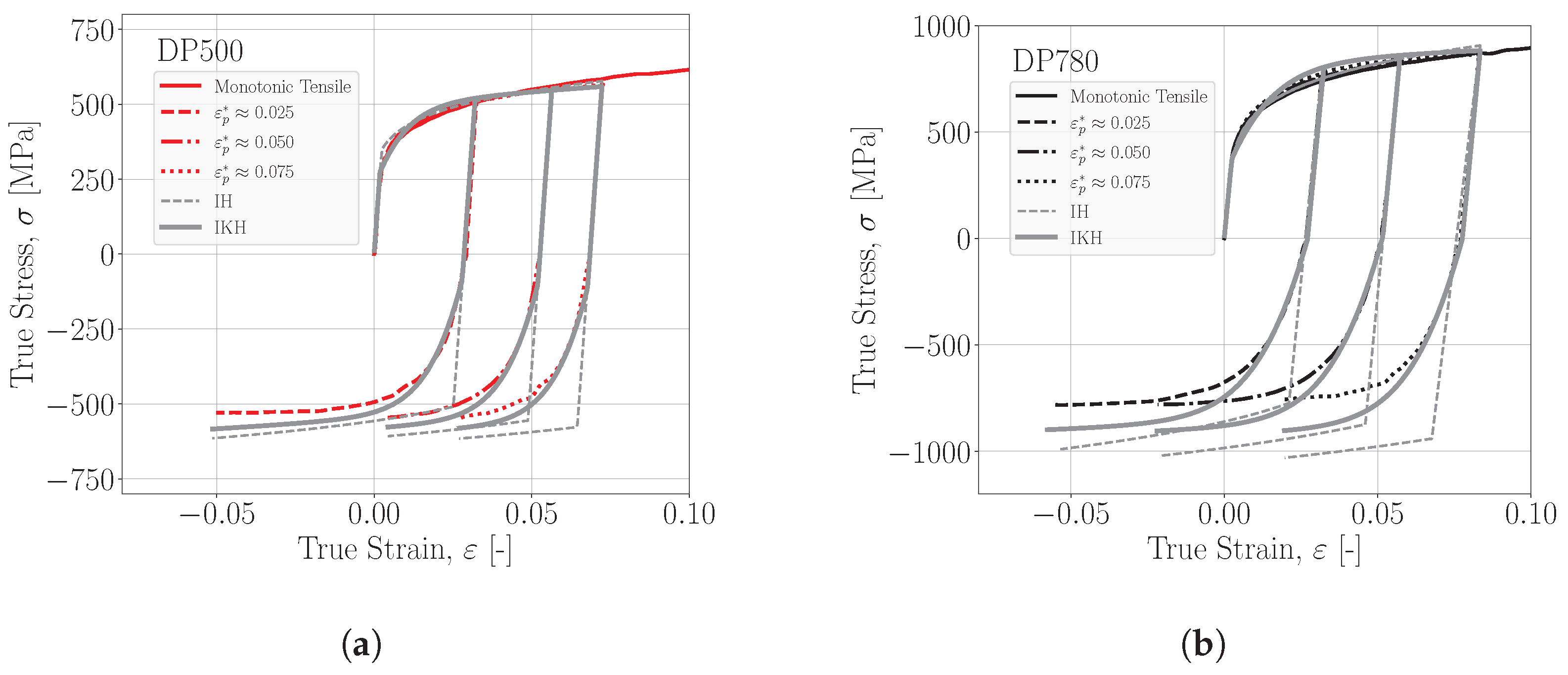
Figure 1 compares the experimental stress–strain curves with the numerical predictions obtained using the isotropic hardening (IH) and combined isotropic–kinematic hardening (IKH) models for the DP500 and DP780 steels. The experimental curves exhibit a pronounced transient Bauschinger effect immediately after load reversal, together with work-hardening stagnation and permanent softening. As expected, the IH model is unable to reproduce the Bauschinger effect, consistently overestimating the stress during reverse loading, particularly in the early stages of strain reversal. In contrast, the IKH model captures the transient Bauschinger effect and provides a closer prediction of the yield stress under reverse loading. Nevertheless, it still fails to fully reproduce the experimentally observed work-hardening stagnation and permanent softening.

2.3. Reverse Bending Test

The identification of constitutive models incorporating kinematic hardening requires experimental tests capable of inducing strain-path reversals and activating the Bauschinger effect. Several experimental techniques have been proposed for this purpose, including uniaxial tension–compression tests, reverse shear tests, and reverse bending tests [48]. Each method offers distinct advantages regarding stress state, achievable strain levels, specimen preparation, and experimental complexity, and no single technique has become the standard approach for constitutive parameter identification.

Among these techniques, reverse bending has attracted increasing attention because it closely reproduces the deformation paths encountered in sheet metal forming operations, where the material experiences successive bending and unbending over tool radii [49]. Unlike uniaxial tension–compression tests, reverse bending naturally generates strain-path reversals under realistic forming conditions while accounting for the through-thickness strain gradients characteristic of bending deformation. Consequently, several reverse bending configurations have been proposed over the last few decades. Yoshida et al. [50] first introduced a cyclic bending apparatus, which was later extended to three-point bending configurations by Geng et al. [51] and subsequently refined by Omerspahic et al. [52]. More recently, Zang et al. [53] proposed a pre-strained three-point bending methodology to characterize the Bauschinger effect without requiring cyclic loading.

Although reverse bending does not provide a direct uniaxial stress–strain response, its load–displacement or moment–curvature curves contain sufficient information to identify constitutive parameters through inverse analysis [53]. This capability, together with its close resemblance to industrial sheet metal forming conditions, makes reverse bending particularly well suited for constitutive model identification and for the machine learning framework proposed in the present work. Building upon the experimental configuration proposed by Omerspahic et al. [52], a new reverse bending apparatus was developed for this work to provide a robust and repeatable experimental setup for the characterization of cyclic bending behavior and the validation of the proposed machine learning framework. In the original configuration, the specimen is supported by three pairs of rollers. The two outer roller pairs are free to rotate while constrained against translational motion, whereas the central roller pair applies the cyclic vertical displacement. This arrangement enables controlled bending–unbending cycles with high repeatability.

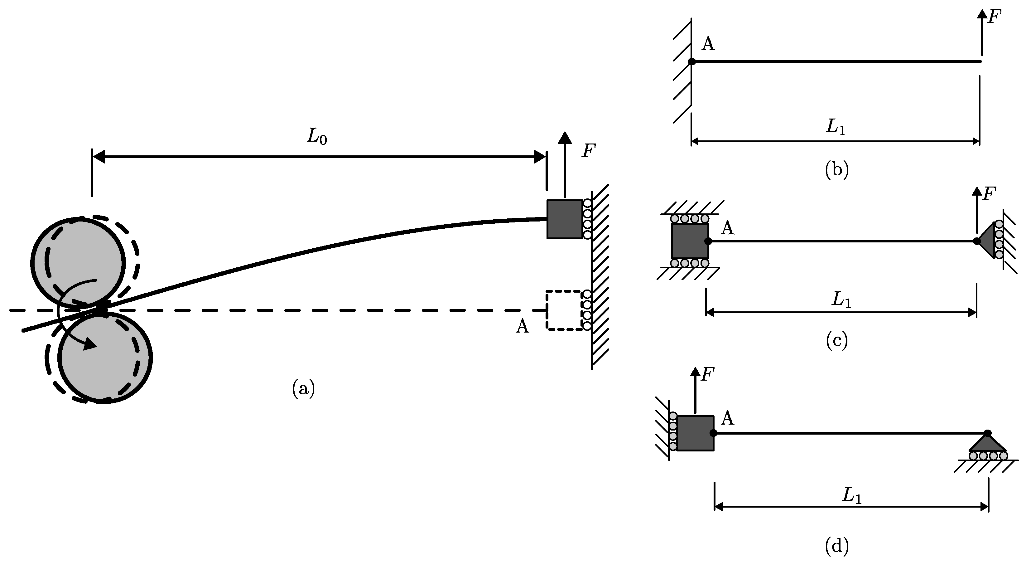
For the numerical modeling of this test, the equivalent non-contact formulation proposed by Zhao and Lee [54] can be adopted. The corresponding boundary conditions are illustrated in Figure 2a. Exploiting the symmetry of the setup, Zhao and Lee demonstrated that the original contact model can be replaced by equivalent non-contact configurations (Figure 2b–d) while preserving the bending moment at the fixed end. These simplified models substantially reduce the computational cost associated with contact simulations. Following their recommendation, the effective length of the non-contact model was taken as $L_1=1.03L_0$.

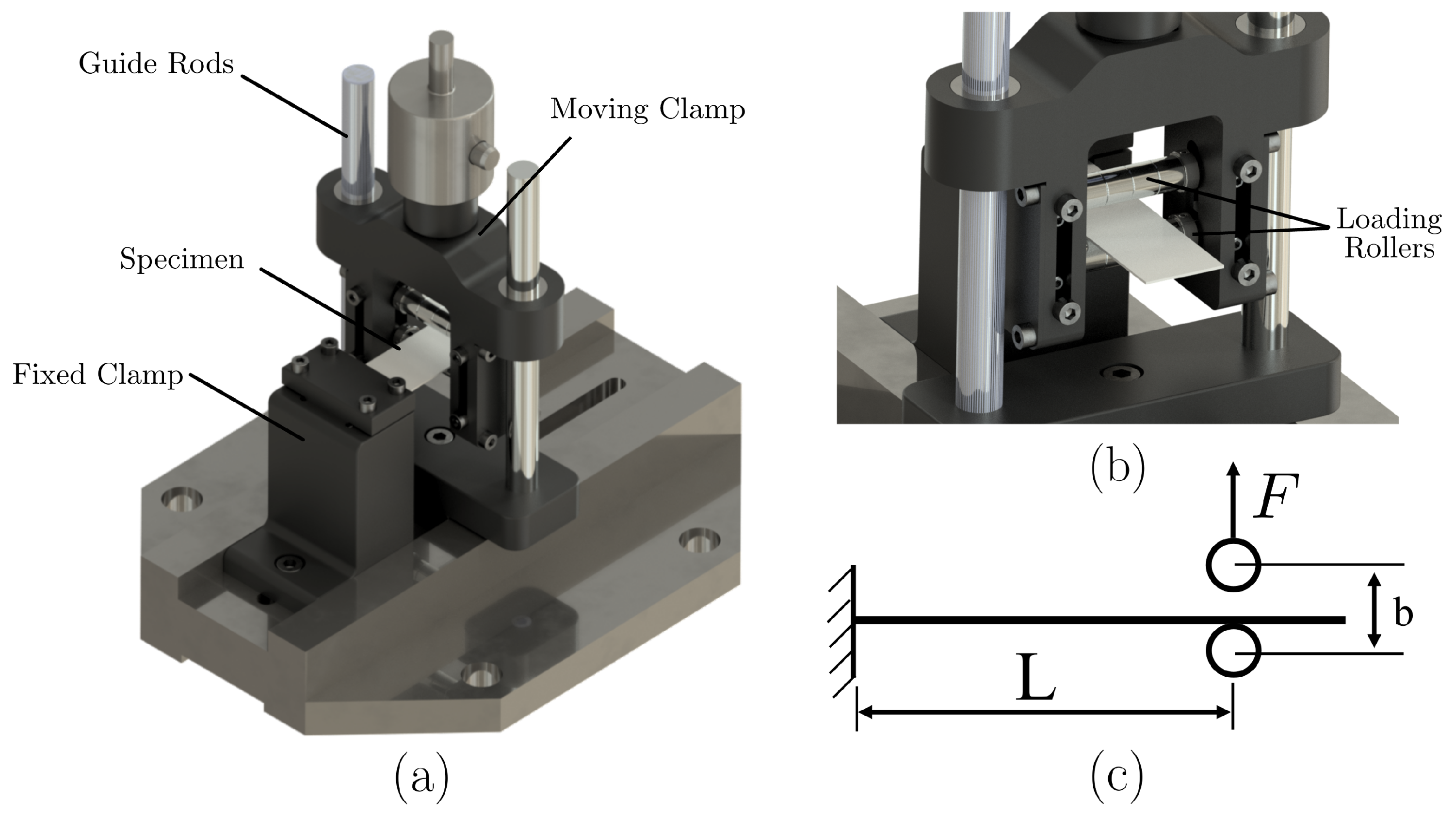
Based on the equivalent non-contact formulation proposed by Zhao and Lee [54], a reverse bending apparatus was developed for the present work. The experimental configuration is illustrated in Figure 3. A rectangular sheet specimen is clamped at one end, while cyclic vertical displacements are applied through two rollers located at a distance L from the clamped edge. The main geometric parameters governing the test are the loading distance L and the roller spacing b. During the test, the specimen is subjected to successive bending and unbending cycles by imposing prescribed vertical displacements $d_i$, thereby generating repeated strain-path reversals representative of industrial sheet metal forming operations.

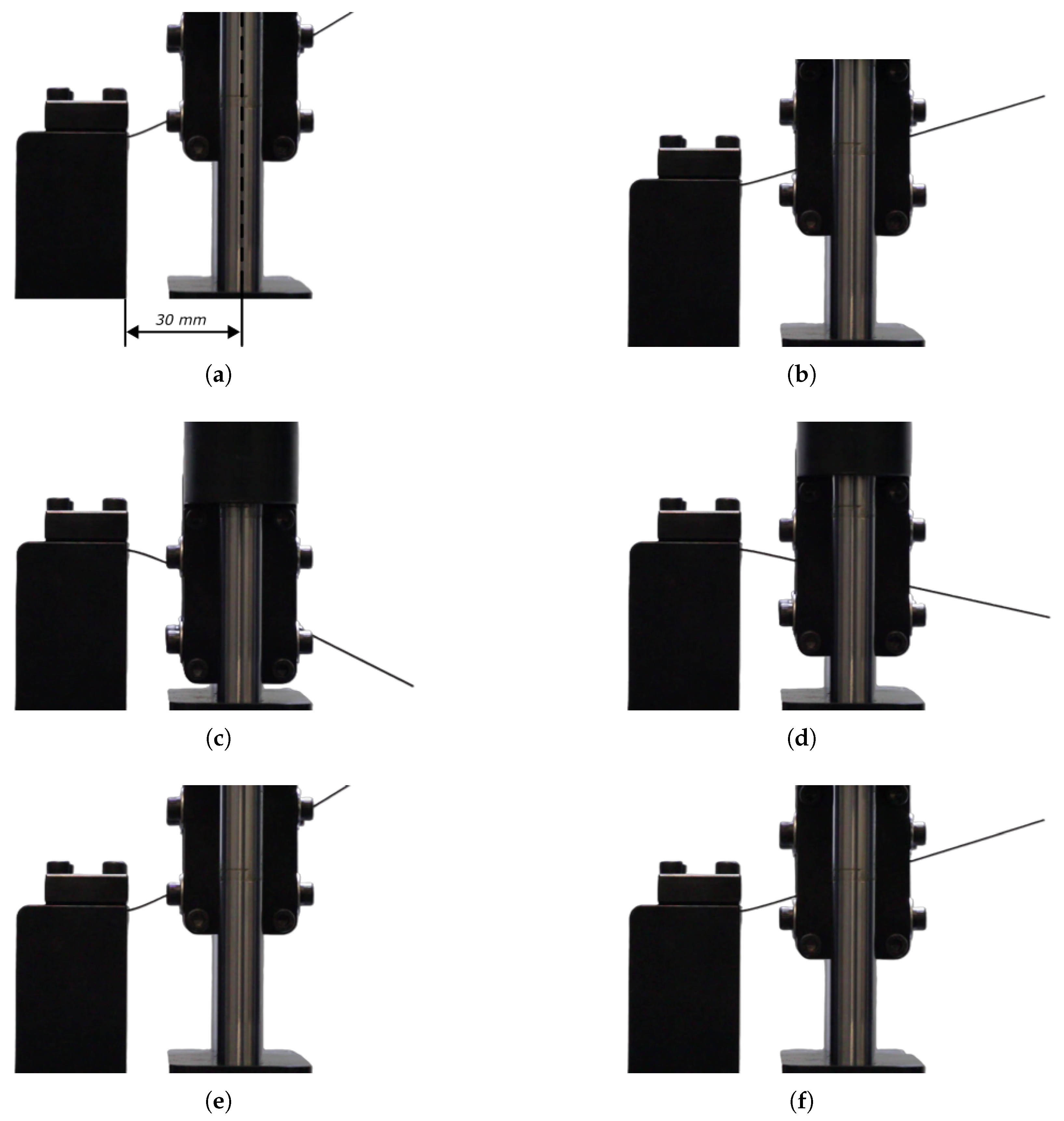
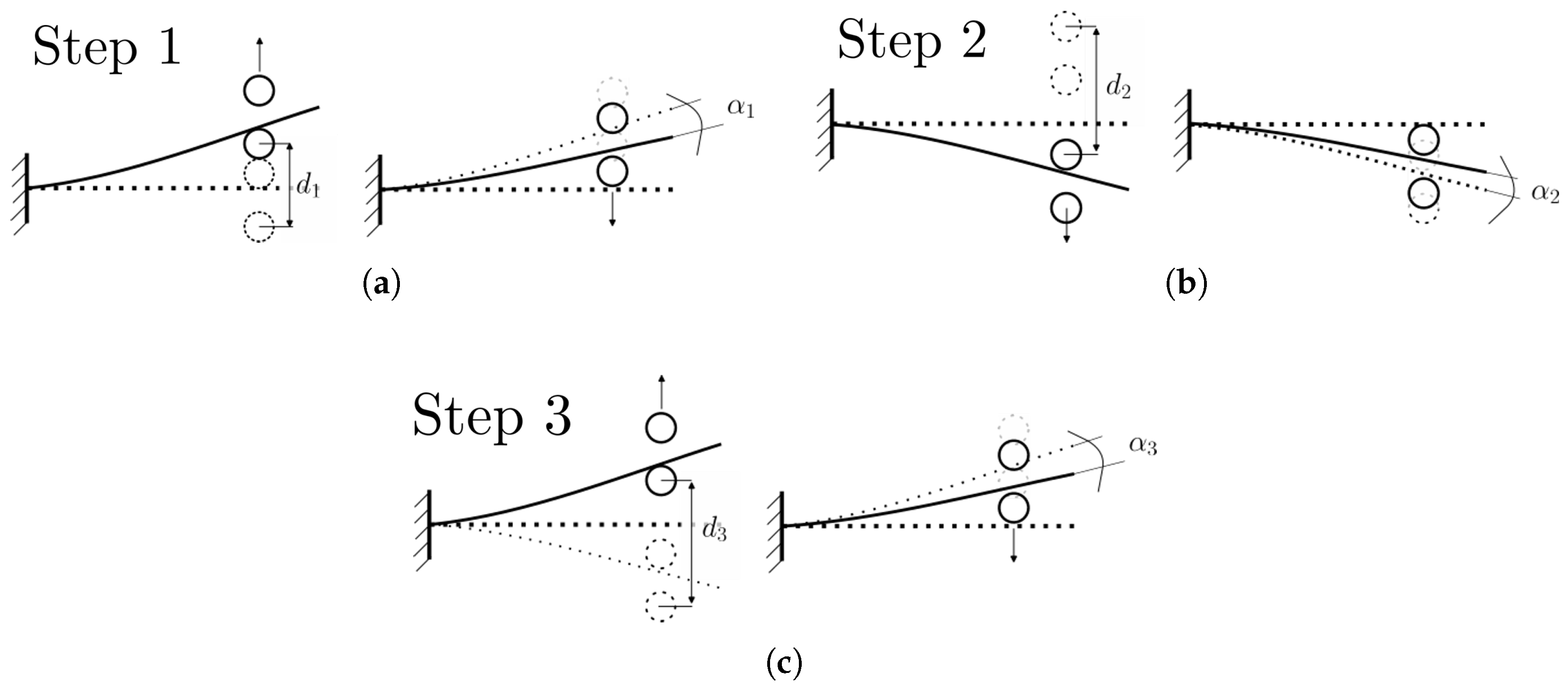
The roller spacing b allows the specimen to recover elastically after each loading stage, enabling the measurement of the corresponding springback angle ${\alpha }_i$. As illustrated in Figure 4, the test consists of a sequence of prescribed displacements ($d_1,d_2,\dots ,d_n$). Each loading stage is followed by unloading until contact between the specimen and the roller are lost, at which point the springback angle is measured. Reversing the loading direction alternately subjects the upper and lower surfaces of the sheet to tension and compression, producing successive strain-path reversals and repeated activation of the Bauschinger effect. Although three loading stages ($n=3$) are considered in the present work, the methodology is readily extendable to an arbitrary number of bending–unbending cycles.

2.3.1. Experimental Testing Condition

To evaluate the behavior of the dual-phase steels (DP500 and DP780), the developed experimental setup was mounted on an Instron universal testing machine model 5900R 300 kN (Norwood, MA, USA), using a 1 kN load cell. During the test, force and displacement data were recorded from the moving crosshead at a sampling rate of 10 Hz. In addition, images were taken during the test to measure the springback angle at each stage. A representation of these images is shown in Figure 5 for the DP500 material. In this figure, each row shows the images at the end of each stage: the left image shows the specimen before elastic recovery and the right image shows it after elastic recovery. Three bending–unbending stages ($n=3$) were performed. A punch displacement of 20 mm was prescribed in the first stage, while the subsequent stages involved a peak-to-peak displacement range of 40 mm, with the punch moving between +20 mm and −20 mm. Rectangular specimens (145 × 30 mm) were manufactured by electrical discharge machining (EDM) along the rolling direction of the sheet, and five specimens were tested for each material to assess repeatability. The geometric parameters were fixed at $L=30$ mm and $b=10$ mm.

2.3.2. Finite Element Model

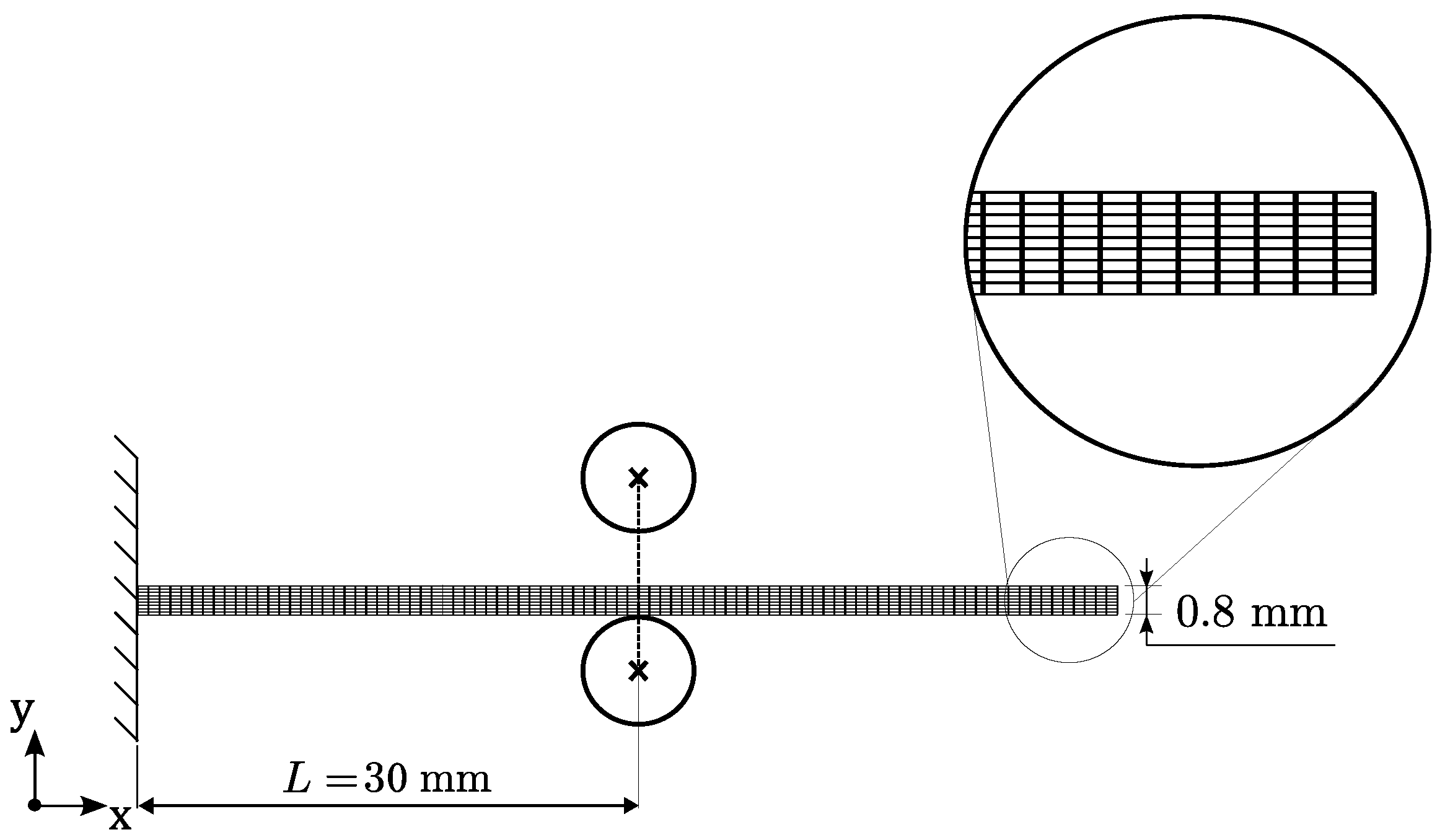
A finite element model was developed to reproduce the proposed reverse bending test. The numerical model serves two main purposes: (i) to validate the numerical representation of the experimental setup against experimental measurements and (ii) to generate the synthetic dataset required for training the proposed machine learning models. Figure 6 schematically illustrates the finite element model considered for the reverse bending test, highlighting its key variables of interest. The model was developed using the Abaqus/Standard finite element code v.2024. The tools were modeled as fully rigid analytical surfaces and the analysis was performed under plane strain conditions, since the specimen width is sufficiently large relative to its thickness. The blank was discretized with 9 layers through thickness using 912 deformable four-node solid elements (type CPE4R from the Abaqus library). The Coulomb friction coefficient was set to 0.1 and the material behavior of the blank was modeled as elastoplastic. The isotropic von Mises yield criterion was adopted, while in-plane anisotropy was not considered. The elastic constants of the material were defined as $E=210\mathrm{GPa}$ and $\nu =0.3$. The boundary conditions fixed the left side of the blank while applying displacement to the rollers on the right side. The material thickness was set to 0.8 mm.

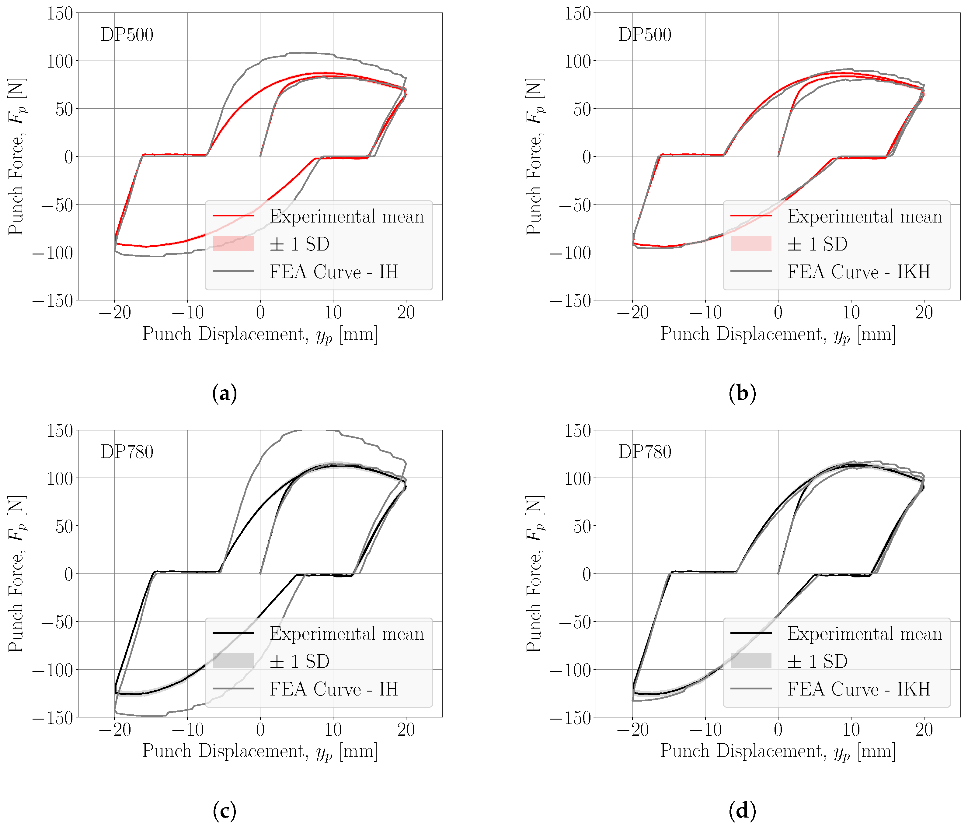
In this numerical model, the effective length L was calibrated using the average experimental reverse bending curve of the DP780 steel. The calibration was performed by minimizing the mean squared error between the experimental and finite element force–displacement responses over the monotonic portion of the experimental curve. The Swift isotropic hardening parameters listed in Table 2 were used. The resulting calibrated value of L was subsequently used for the DP500 steel. Figure 7 shows the comparison between the mean experimental and FEA force–displacement ($F_p$–$y_p$) curves for the two materials. The shaded regions represent ± one standard deviation obtained from five independent experimental tests.

As expected, the isotropic hardening model captures the bending behavior only prior to the onset of inversion. Once inversion occurs (steps 2 and 3), the finite element model is unable to fully reproduce the experimental behavior and tends to overestimate the force values. On the other hand, when considering a combined isotropic–kinematic model, the experimental and numerical curves tend to converge, as observed in Figure 7b,d for DP500 and DP780, respectively. In this case, the combined isotropic–kinematic hardening parameters (IKH) shown in Table 3 were used. However, the agreement is still not perfect, indicating that the set of parameters identified from the tension–compression test may not fully capture the material behavior under bending loads.

3. Machine Learning Framework

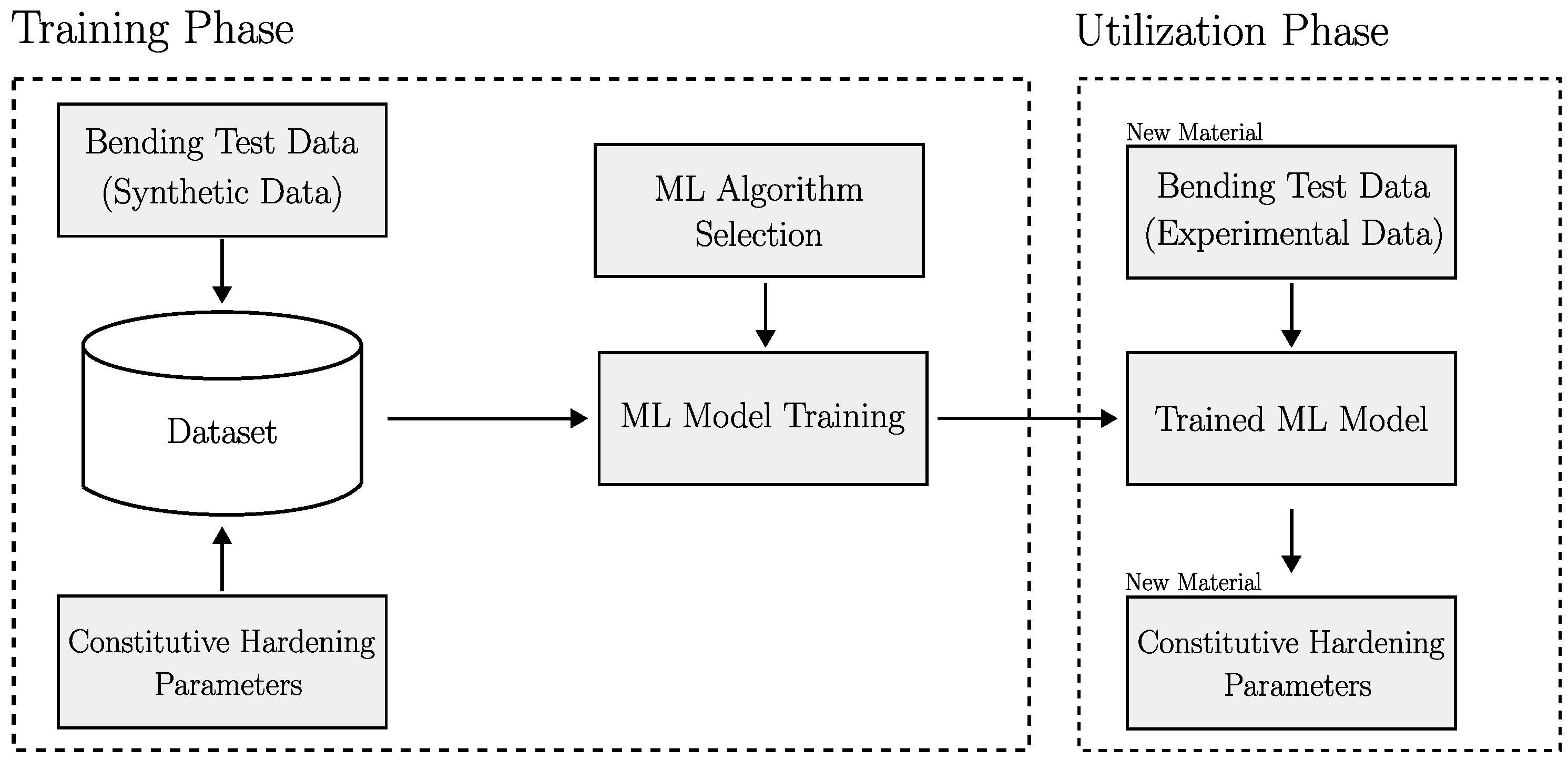
The proposed framework combines reverse bending experiments, finite element simulations and deep learning to identify constitutive hardening parameters directly from force–displacement curves. The overall workflow is illustrated in Figure 8 and consists of two stages. In the training phase, a synthetic dataset is generated through finite element simulations using different combinations of constitutive parameters. The resulting force–displacement curves are then used to train a machine learning model capable of learning the relationship between the mechanical response and the corresponding material parameters. Once trained, the model can be applied directly to experimental reverse bending data. In this application phase, the network predicts the constitutive parameters without requiring iterative finite element simulations or optimization procedures, providing a fast alternative to conventional inverse identification techniques.

3.1. Synthetic Dataset Generation

The neural network was trained using a synthetic dataset generated from finite element simulations of the reverse bending test presented in Section 2.3.2. Each simulation corresponds to a unique combination of constitutive parameters and produces a force–displacement curve used as input to the neural network. The constitutive parameters were systematically varied within the ranges listed in

Table 4. Parameter ranges adopted for generating the synthetic dataset of the combined isotropic–kinematic hardening (IKH) model.

Parameter	Symbol	Range
Isotropic Hardening (Swift)
Strength coefficient	K [MPa]	400–1600
Offset strain	${\epsilon }_0$	0.0001–0.01
Hardening exponent	n	0.05–0.35
Kinematic Hardening (Armstrong–Frederick)
Kinematic modulus	C [MPa]	1000–100,000
Decay rate	$\gamma$	0–500
Elastic Properties
Young’s modulus	E [GPa]	210 (fixed)
Poisson’s ratio	$\nu$	0.3 (fixed)

. The selected parameter ranges were defined based on values reported in the literature, particularly the work of Silvestre et al. [55], which characterized the combined isotropic–kinematic hardening response of materials ranging from mild steels to advanced high-strength steels. Although the synthetic dataset was generated by sampling ${\epsilon }_0$, the machine learning model was trained to predict the corresponding initial yield stress, ${\sigma }_0$, computed from Equation (2). Using ${\sigma }_0$ instead of ${\epsilon }_0$ provides a more directly interpretable representation of the initial yielding behavior. Consequently, the network predicts the parameter set $(K,{\sigma }_0,n,C,\gamma )$.

A total of 5000 combinations were generated using Sobol sampling [56], with a random seed of 10, and the corresponding finite element simulations were subsequently performed for each combination. Compared with purely random sampling, Sobol sequences provide a more uniform coverage of the five-dimensional parameter space defined by the independently sampled parameters K, ${\epsilon }_0$, n, C, and $\gamma$, while reducing clustering effects. The initial yield stress ${\sigma }_0$ was not sampled independently, but calculated from K, ${\epsilon }_0$, and n according to Equation (2). The resulting ${\sigma }_0$ values ranged from 50 to 1200 MPa.

The complete simulation workflow was automated, using scripts developed in Python 3.10.16, which generated the Abaqus input files, assigned the constitutive parameters, submitted the finite element analyses, and extracted the corresponding force–displacement responses from the output database. This automated procedure enabled the efficient generation of the entire dataset while minimizing manual intervention and ensuring consistency across all simulations. Each finite element simulation required approximately 20 s on average on a computer equipped with an Intel(R) Core(TM) i9-9900K CPU @ 3.60 GHz, 64.0 GB of RAM, and an NVIDIA Quadro P620 graphics card, resulting in a total computational time of approximately 27.8 h for the 5000 simulations.

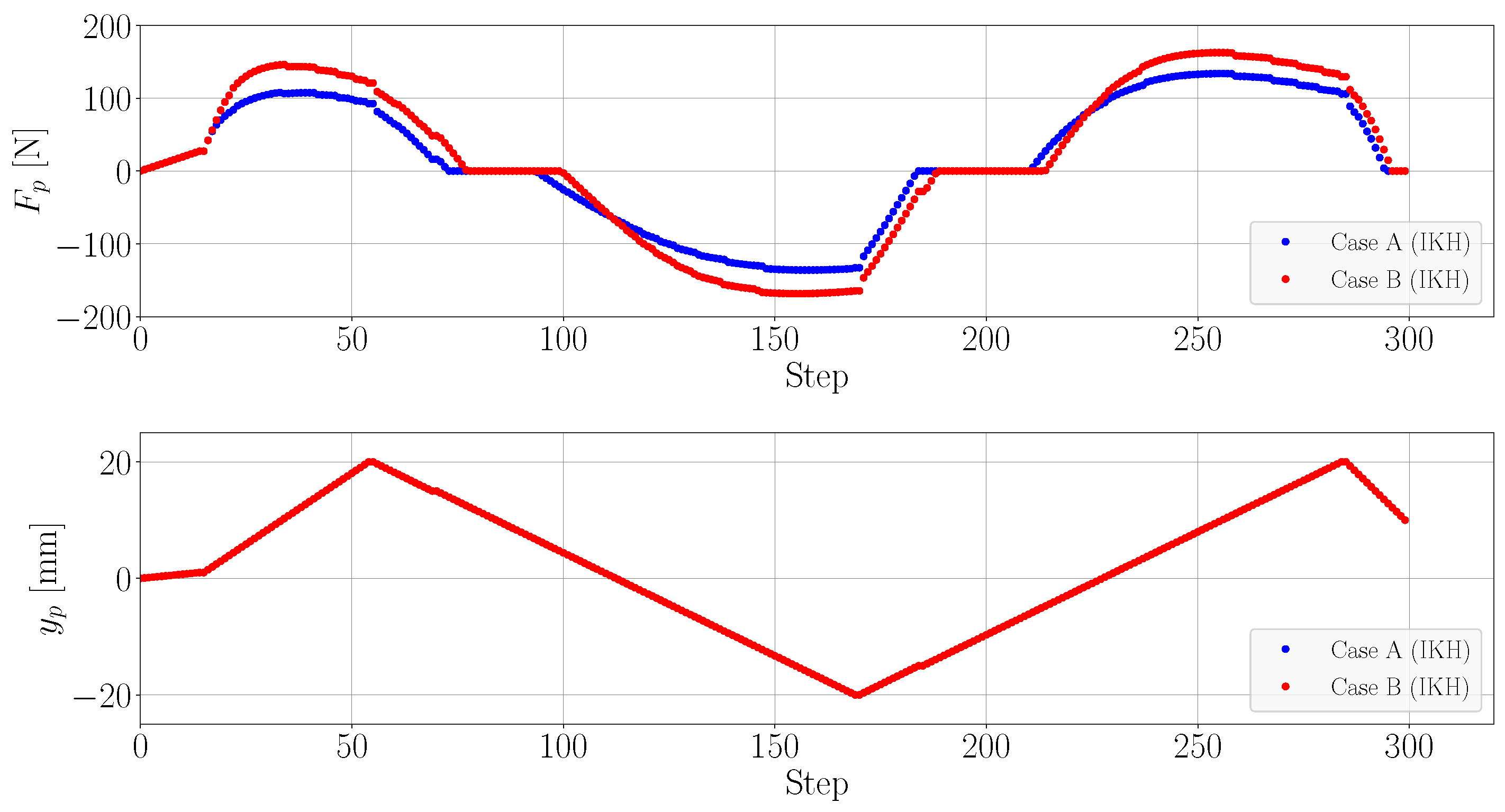
Representative force–displacement responses from the synthetic dataset are shown in Figure 9. The curves correspond to two representative material parameter combinations (Cases A and B) spanning the design space, whose constitutive parameters are summarized in

Table 5. Representative material parameter combinations (Cases A and B) selected from the synthetic dataset.

Case	K [MPa]	${\mathit{\sigma }}_0$ [MPa]	n	C [MPa]	$\mathit{\gamma }$
A	1000	346.8	0.20	50500	250
B	988	599.6	0.10	67708	346

. Each response consists of 300 sampling points covering the complete bending–unbending sequence, including loading, unloading, and reverse loading. These sequential force–displacement histories constitute the input sequences to the proposed LSTM network.

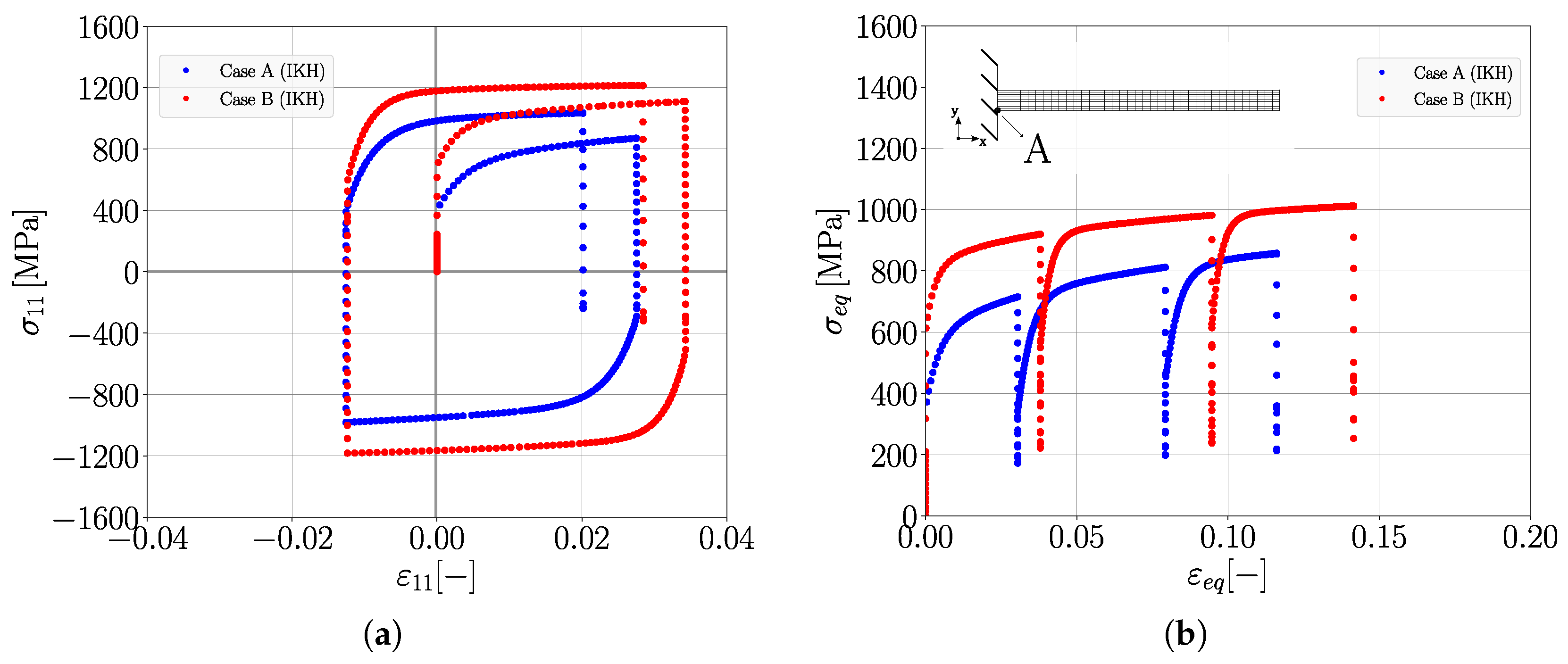
To further illustrate the mechanical response generated by the reverse bending test, Figure 10a presents the evolution of the longitudinal stress ${\sigma }_{11}$ as a function of the longitudinal strain ${\epsilon }_{11}$, for the two representative synthetic dataset cases, at Point A, located on the lower surface of the sheet near the clamped end. Figure 10b shows the corresponding equivalent stress–strain response based on the von Mises yield criterion. Considering the complete synthetic dataset, during the first bending stage, Point A is subjected to tensile loading and reaches an equivalent plastic strain between approximately 0.03 and 0.05. Following load reversal, the stress state changes from tension to compression, and the equivalent strain increases to approximately 0.10. During the third stage, Point A returns to tension and the accumulated equivalent plastic strain reaches approximately 0.15, with some material configurations reaching accumulated equivalent strains approaching 0.20. These results show that the proposed reverse bending test produces repeated stress reversals together with significant accumulated plastic deformation, providing rich information for identifying constitutive models incorporating kinematic hardening.

3.2. Training Strategy

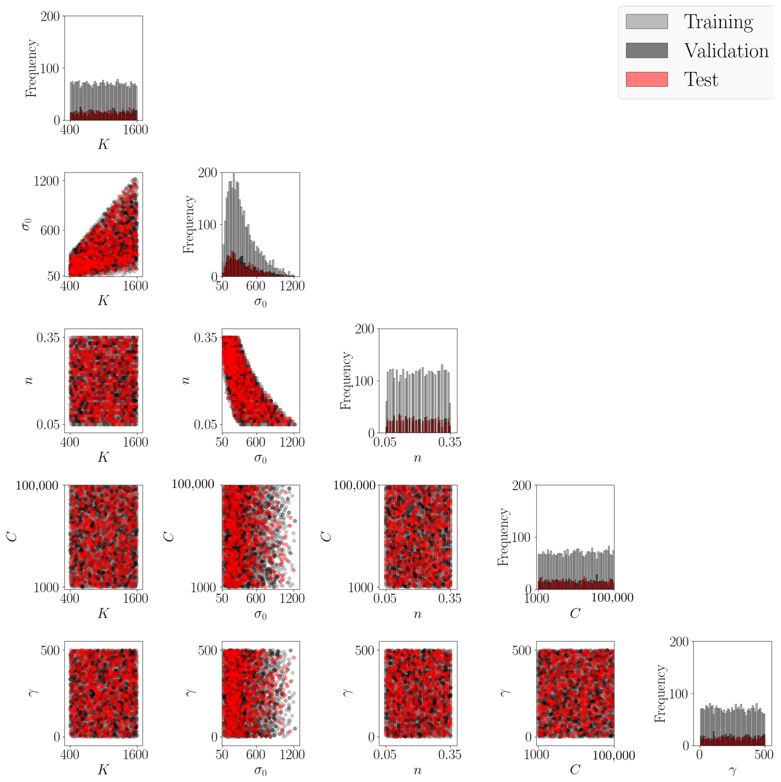
The resulting dataset, obtained from the selected 5000 finite element simulations, was divided into training (70%), validation (15%), and test (15%) datasets. The training dataset was used to optimize the network weights, the validation dataset to monitor the learning process, tune the hyperparameters, and prevent overfitting, and the test dataset was reserved for an independent evaluation of the final model performance. The corresponding parameter distributions are presented in Figure 11. The histograms confirm that Sobol sampling provides a nearly uniform coverage of the selected parameter space defined by the independently sampled parameters K, ${\epsilon }_0$, n, C, and $\gamma$, and that the three datasets exhibit similar statistical distributions. As ${\sigma }_0$ is a derived quantity, its distribution is not expected to be uniform.

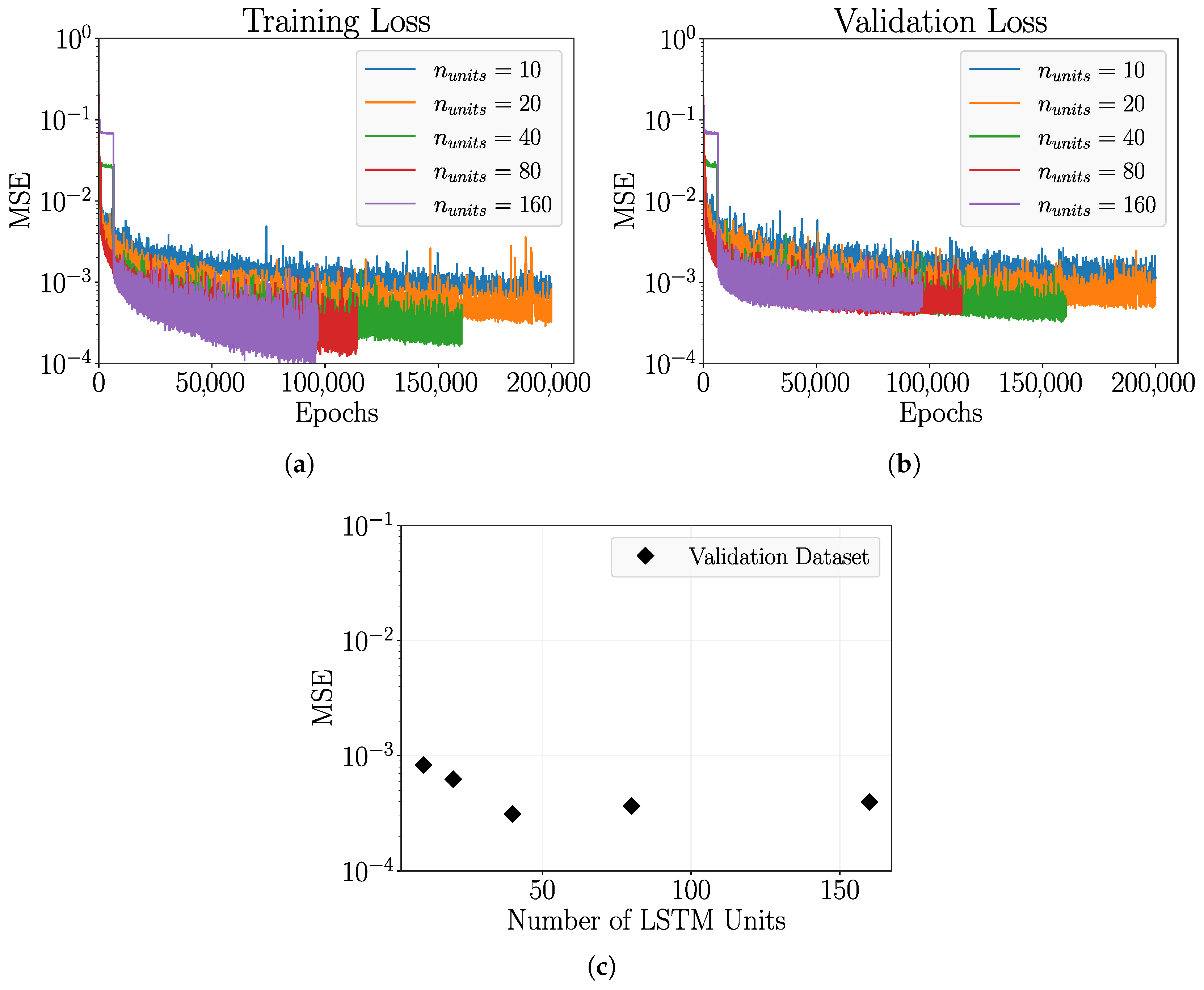
Prior to training, both the input force–displacement sequences and the output constitutive parameters were normalized to the interval $[-1,1]$ to improve numerical stability and facilitate the optimization process. To capture the sequential nature of the force–displacement curves, a bidirectional long short-term memory (Bi-LSTM) network [57,58] was adopted. Unlike a conventional multilayer perceptron (MLP), which treats the input as a set of static features and does not explicitly account for their sequential ordering, the Bi-LSTM directly processes the complete ordered force–displacement sequence without requiring explicit feature selection. Compared with a conventional LSTM, the bidirectional architecture processes the sequence in both forward and backward directions, allowing information from different portions of the loading response to be interpreted in the context of the complete loading history. Since the network performance depends strongly on the selected hyperparameters, a preliminary sensitivity analysis was conducted to determine the appropriate number of Bi-LSTM units. Five network configurations comprising 10, 20, 40, 80, and 160 Bi-LSTM units were evaluated while maintaining a constant learning rate of 0.001. An early stopping criterion was employed during training, with a maximum of 200,000 training epochs. Each network configuration was stopped independently when the validation loss did not improve for 1000 consecutive epochs. The corresponding training and validation histories are presented in Figure 12a and Figure 12b, respectively, whereas Figure 12c summarizes the minimum validation loss together with the corresponding test loss for each configuration.

As expected, increasing the number of Bi-LSTM units substantially reduces the training loss, indicating an enhanced ability to capture the nonlinear relationship between the force–displacement response and the constitutive parameters. A similar trend is observed for the validation dataset, demonstrating improved generalization to previously unseen data. However, beyond approximately 40 Bi-LSTM units, the reduction in prediction error becomes marginal despite the increased model complexity. As shown in Figure 12c, the network with 40 Bi-LSTM units achieves the lowest validation error and was therefore selected for all subsequent analyses.

Following the selection of the network architecture, an extended hyperparameter search was performed, using Bayesian optimization, to determine the remaining training parameters. The Adam optimizer was employed together with an exponentially decaying learning rate, starting from an initial value of 0.01, to promote stable convergence during the early stages of training while allowing finer parameter updates as optimization progressed. In addition, an early stopping criterion was adopted to terminate the training process when no further improvement was observed on the validation dataset. The final hyperparameters are summarized in

Table 6. Final hyperparameters of the proposed Bi-LSTM network.

Hyperparameter	Value
Architecture	Bidirectional LSTM
Bi-LSTM units	40
Output layer	Dense (5 neurons)
Optimizer	Adam
Initial learning rate	0.01
Learning-rate scheduler	Exponential decay
Decay rate	0.96
Decay steps	1000
Batch size	64
Maximum epochs	200,000
Loss function	Mean Squared Error
Hyperparameter optimization	Bayesian optimization

. The final Bi-LSTM model required approximately 8 h for training on the same computational workstation. Once trained, the model required approximately 0.2 s to infer the five constitutive parameters from a single force–displacement curve.

3.3. Prediction Performance

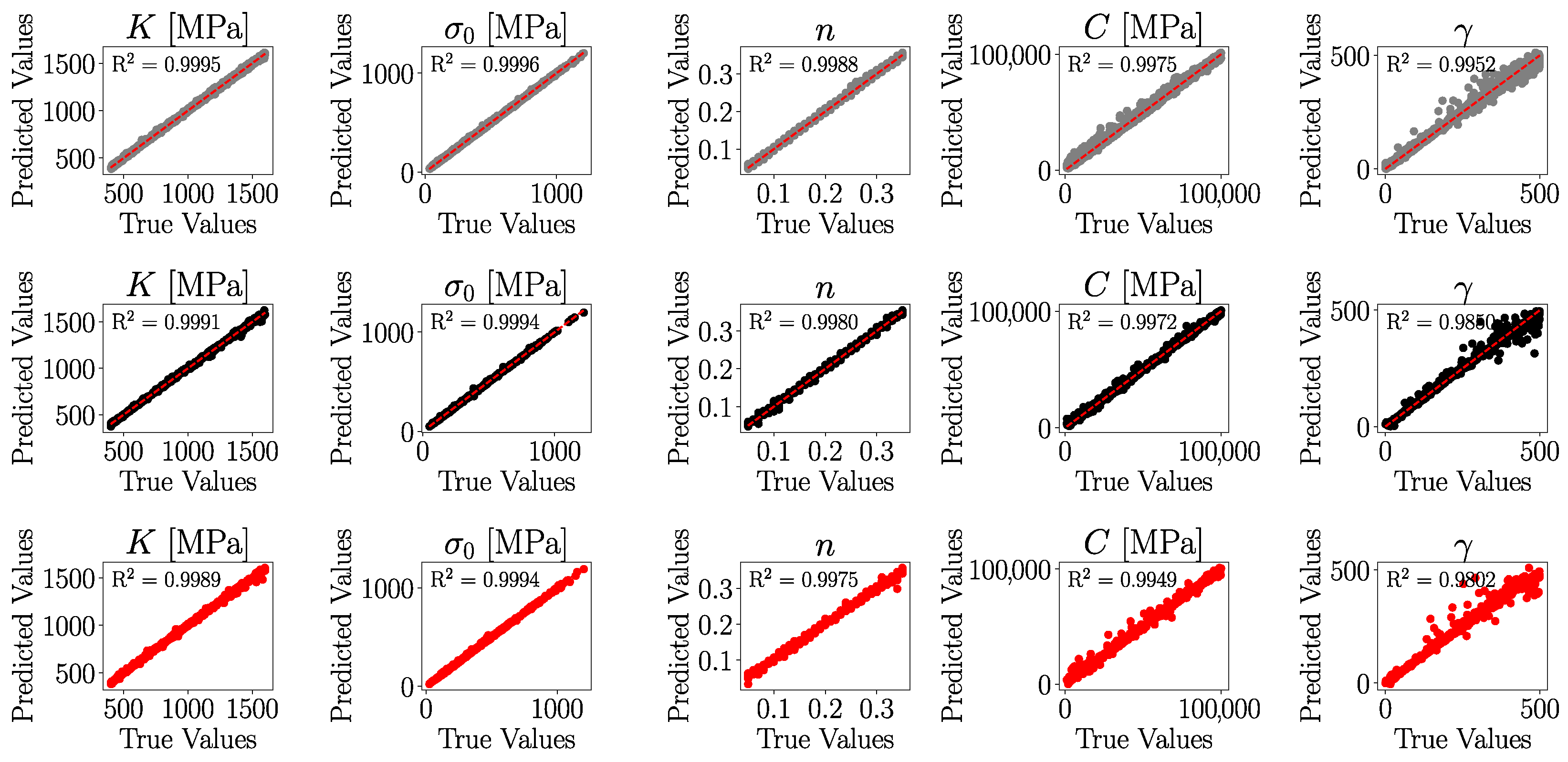
The performance of the trained model was evaluated using the training, validation, and test datasets. Figure 13 compares the predicted and target constitutive parameters for each dataset and shows the coefficients of determination ($R^2$) for each variable. The ($R^2$) values are close to unity for all five parameters, indicating a strong agreement between the predicted and target values. The similar performance observed across the training, validation, and independent test datasets indicates that the trained network generalizes well to previously unseen simulations. Among the five parameters, the isotropic hardening parameters (K, ${\sigma }_0$ and n) are predicted with consistently high accuracy, whereas the kinematic hardening parameters (C and $\gamma$) exhibit slightly larger scatter. The largest deviation is observed for $\gamma$, for which the coefficient of determination remains above 0.98 in the test dataset. Overall, the results indicate consistent prediction performance across the five constitutive parameters, with greater variability for the kinematic hardening parameters.

The prediction performance was quantified using the mean absolute error (MAE), root mean squared error (RMSE), and normalized root mean squared error (NRMSE). MAE and RMSE are reported in the physical units of each constitutive parameter, while NRMSE provides a dimensionless measure of the overall prediction error normalized by the corresponding parameter range in the training dataset. The NRMSE is defined as:

$$\mathrm{NRMSE}(\%)={\displaystyle \frac{\mathrm{RMSE}}{y_{\max }^{\mathrm{train}}-y_{\min }^{\mathrm{train}}}}\times 100,$$

(4)

where $y_{\max }^{\mathrm{train}}$ and $y_{\min }^{\mathrm{train}}$ denote the maximum and minimum values of the corresponding constitutive parameter in the training dataset. The resulting prediction errors for the training, validation, and test datasets are summarized in

Table 7. Prediction errors for the material parameters across the training, validation, and test datasets.

Dataset	Parameter	MAE	RMSE	NRMSE (%)
Train	K	5.60	7.67	0.64
	${\sigma }_0$	3.16	4.39	0.37
	n	0.0025	0.0031	1.02
	C	916.92	1439.63	1.46
	$\gamma$	5.61	10.03	2.01
Validation	K	7.02	10.68	0.89
	${\sigma }_0$	3.48	5.56	0.47
	n	0.0029	0.0038	1.26
	C	1020.00	1506.76	1.52
	$\gamma$	8.66	17.80	3.56
Test	K	7.14	11.15	0.93
	${\sigma }_0$	3.76	5.79	0.49
	n	0.0031	0.0044	1.45
	C	1188.96	2041.84	2.06
	$\gamma$	9.31	20.04	4.01

. The results show consistently low prediction errors across the three datasets. In the independent test dataset, the NRMSE remains below 5% for all parameters, with the lowest value obtained for ${\sigma }_0$ (0.49%) and the highest for $\gamma$ (4.01%).

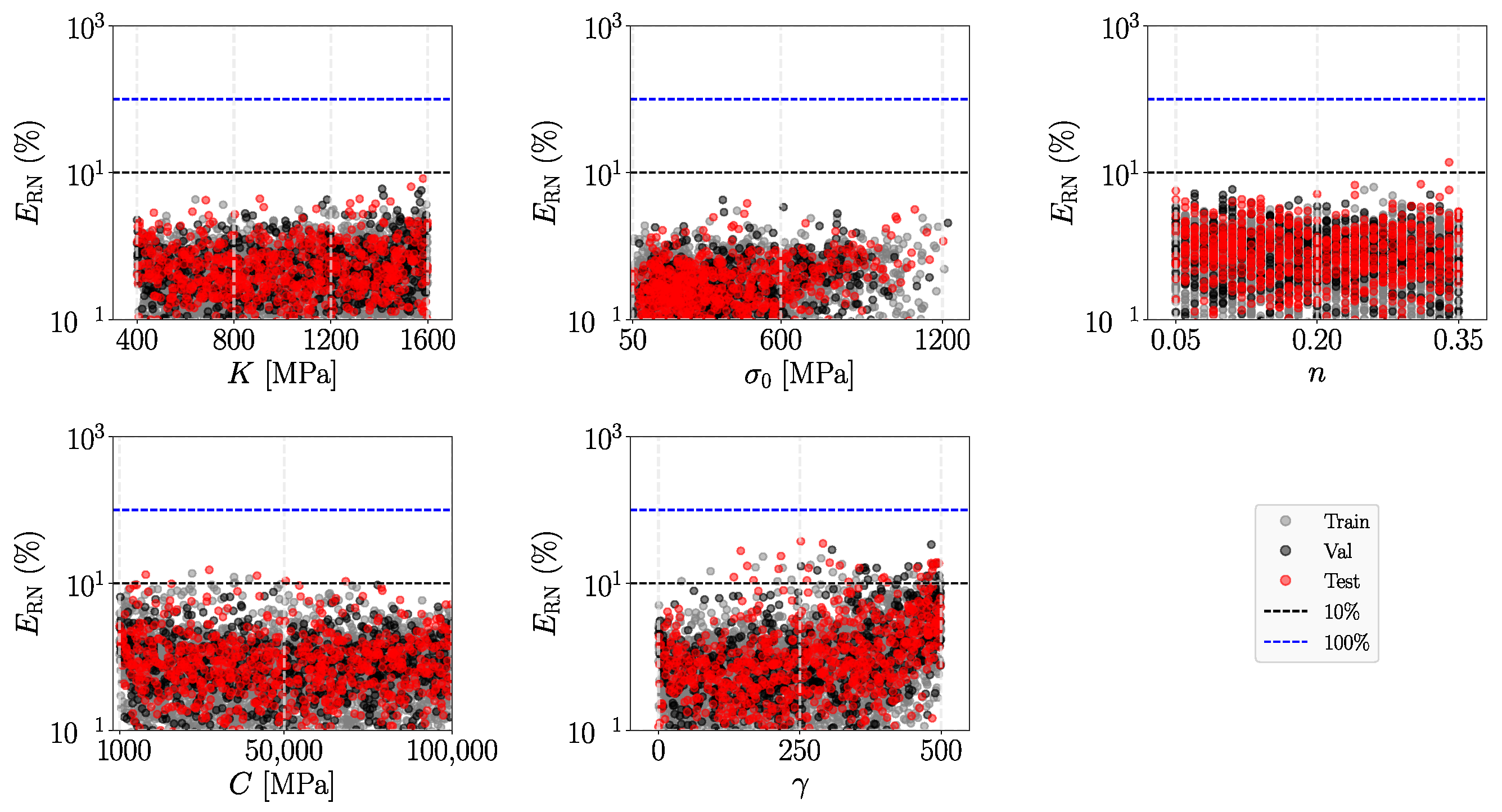
To further analyze how the prediction error varies across the parameter ranges, Figure 14 presents the range-normalized error as a function of the true parameter value for each constitutive parameter. The range-normalized error was calculated as:

$$E_{\mathrm{RN}}(\%)={\displaystyle \frac{\left|\widehat{y}-y\right|}{y_{\max }^{\mathrm{train}}-y_{\min }^{\mathrm{train}}}}\times 100,$$

(5)

where $\widehat{y}$ and y denote the predicted and true values, respectively, and $y_{\max }^{\mathrm{train}}$ and $y_{\min }^{\mathrm{train}}$ are the maximum and minimum values of the corresponding parameter in the training dataset. The error is normalized by the corresponding parameter range in the training dataset, allowing the prediction errors to be compared consistently across parameters with different scales.

The isotropic hardening parameters (K, ${\sigma }_0$, and n) show low prediction errors across their respective ranges, with errors generally below 10%. The kinematic hardening parameters (C and $\gamma$) show a broader distribution of prediction errors, particularly for $\gamma$, where a larger number of predictions exceed the 10% reference level. The maximum error in the test dataset is below 10% for K (8.30%) and ${\sigma }_0$ (3.82%), whereas larger deviations are observed for n, C and $\gamma$, reaching 13.83%, 15.27% and 37.36%, respectively. The largest variability is therefore observed for $\gamma$, indicating that it remains the most challenging parameter to predict accurately. Despite the non-uniform distribution of ${\sigma }_0$ resulting from the sampling strategy, Figure 13 and Figure 14 do not show an evident increase in prediction error towards the lower or higher ${\sigma }_0$ regions.

4. Results

4.1. Effect of Parameter Prediction Errors on the Constitutive Behavior

This section evaluates how prediction errors in the constitutive parameters predicted by the proposed Bi-LSTM model affect the resulting material behavior. First, the overall prediction accuracy is assessed through the distribution of the mean squared error across the training, validation, and test datasets. Since the constitutive parameters have different magnitudes and units, the MSE is computed using the normalized parameter values and is used as a dimensionless metric for comparing prediction performance. Representative prediction cases are then analyzed to investigate the influence of these errors on the resulting material response.

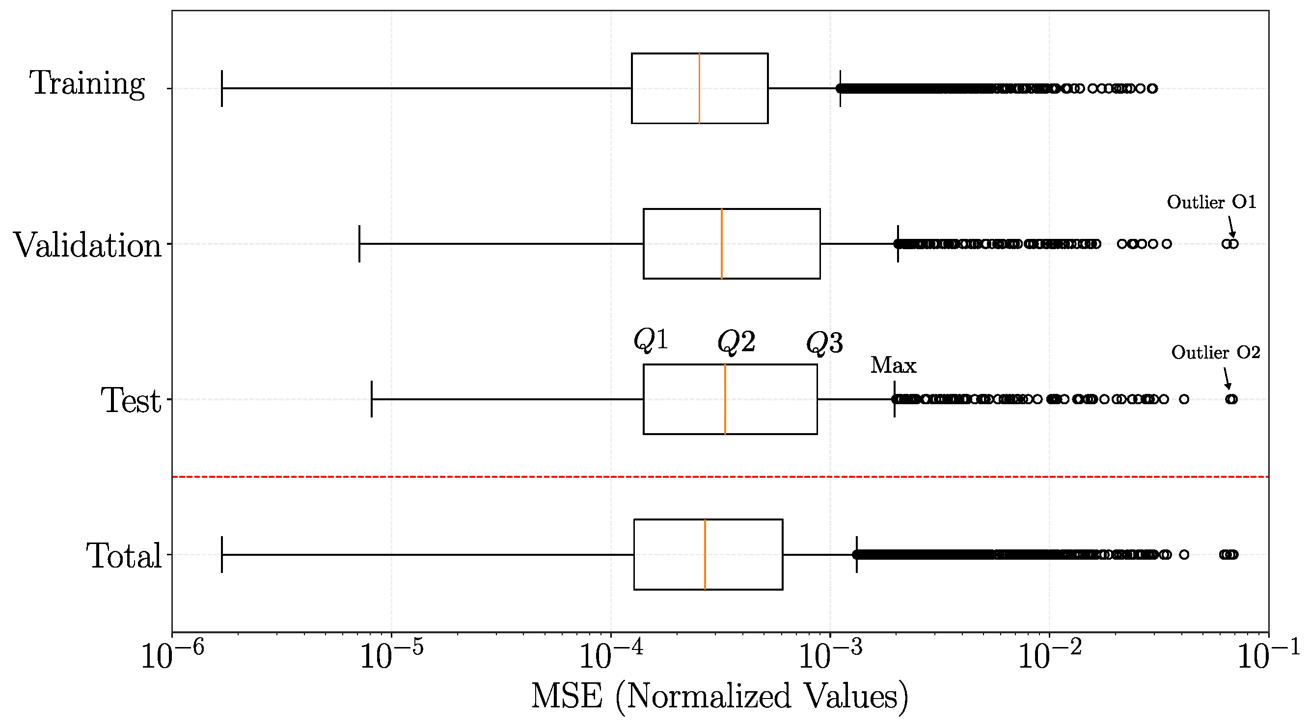
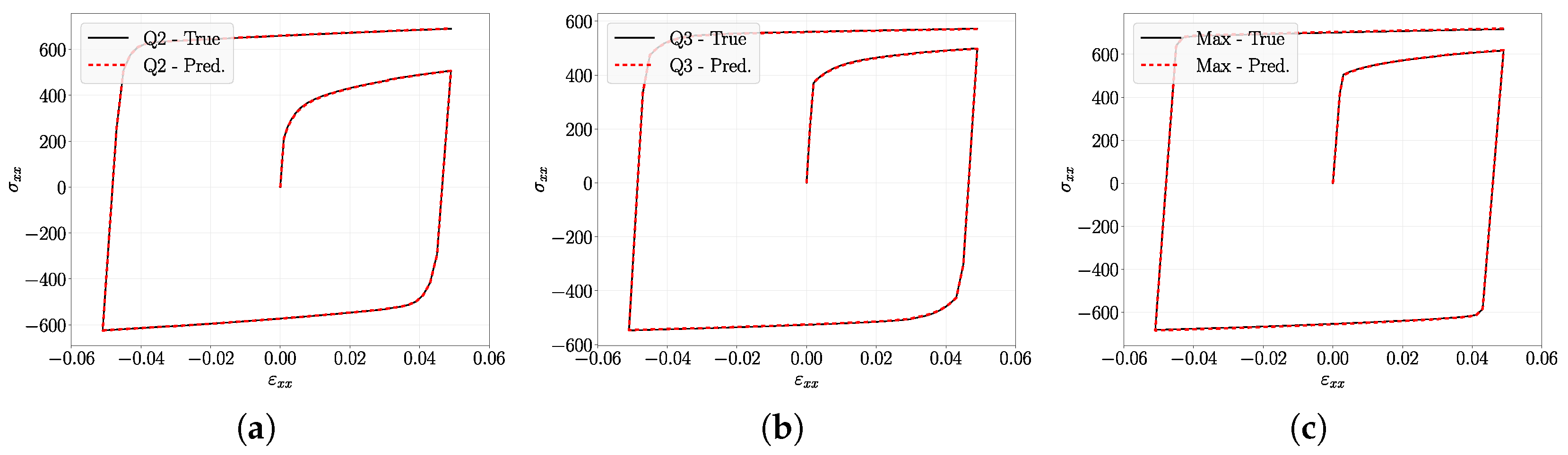
Figure 15 presents the distribution of the MSE computed from the normalized outputs of the network for the five predicted constitutive parameters. The boxplots correspond to the training, validation, test, and complete datasets (5000 simulations). Each boxplot shows the interquartile range (IQR), with the median (Q2) indicated by the central line and the first (Q1) and third (Q3) quartiles by the box boundaries. The whiskers extend to the most extreme values within 1.5 times the IQR, while observations beyond this range are represented as outliers. Based on this distribution, three representative cases from the test dataset are selected for detailed analysis: the median case (Q2), the third-quartile case (Q3), and the case with the maximum non-outlier MSE (Max).

The expected and predicted constitutive parameters for the representative cases are summarized in

Table 8. Expected and predicted parameters for Cases Q2, Q3 and Max, together with the corresponding range-normalized absolute errors, $E_{\mathrm{RN}}$.

Case		K [MPa]	${\mathit{\sigma }}_0$ [MPa]	n	C [MPa]	$\mathit{\gamma }$
Q2	Expected	837.11	220.55	0.23	42,088.87	478.03
	Predicted	842.06	216.87	0.23	40,425.30	472.88
	$E_{\mathrm{RN}}$	0.41%	0.31%	0.00%	1.68%	1.03%
Q3	Expected	600.83	367.35	0.10	10,849.24	213.32
	Predicted	602.28	368.31	0.10	9755.39	202.24
	$E_{\mathrm{RN}}$	0.12%	0.08%	0.00%	1.11%	2.22%
Max	Expected	817.48	499.20	0.10	3586.18	484.25
	Predicted	823.18	496.74	0.10	2283.24	388.40
	$E_{\mathrm{RN}}$	0.48%	0.21%	0.00%	1.32%	19.18%

, together with the corresponding range-normalized absolute errors, $E_{\mathrm{RN}}$ (Equation (5)). The results show that the isotropic hardening parameters (K, ${\sigma }_0$, and n) exhibit consistently small $E_{\mathrm{RN}}$ values across the three representative cases. For the median case (Q2), the $E_{\mathrm{RN}}$ values remain below 0.5% for the isotropic hardening parameters, while the errors for C and $\gamma$ remain below 2%. For the third-quartile case (Q3), the errors remain similarly low, with $E_{\mathrm{RN}}$ values below 2.3% for all parameters. The maximum non-outlier case (Max) shows a more pronounced deviation for $\gamma$, for which $E_{\mathrm{RN}}$ reaches 19.18%, while the corresponding errors for the remaining parameters remain below 1.5%. These results indicate that the larger prediction errors observed in the representative cases are primarily associated with the kinematic hardening parameters, particularly $\gamma$. According to the boxplot criterion, cases with MSE values lying beyond 1.5 times the interquartile range from the corresponding quartile limits are classified as outliers. Based on this criterion, 95 cases (13% of the test dataset) are identified as outliers and are further investigated.

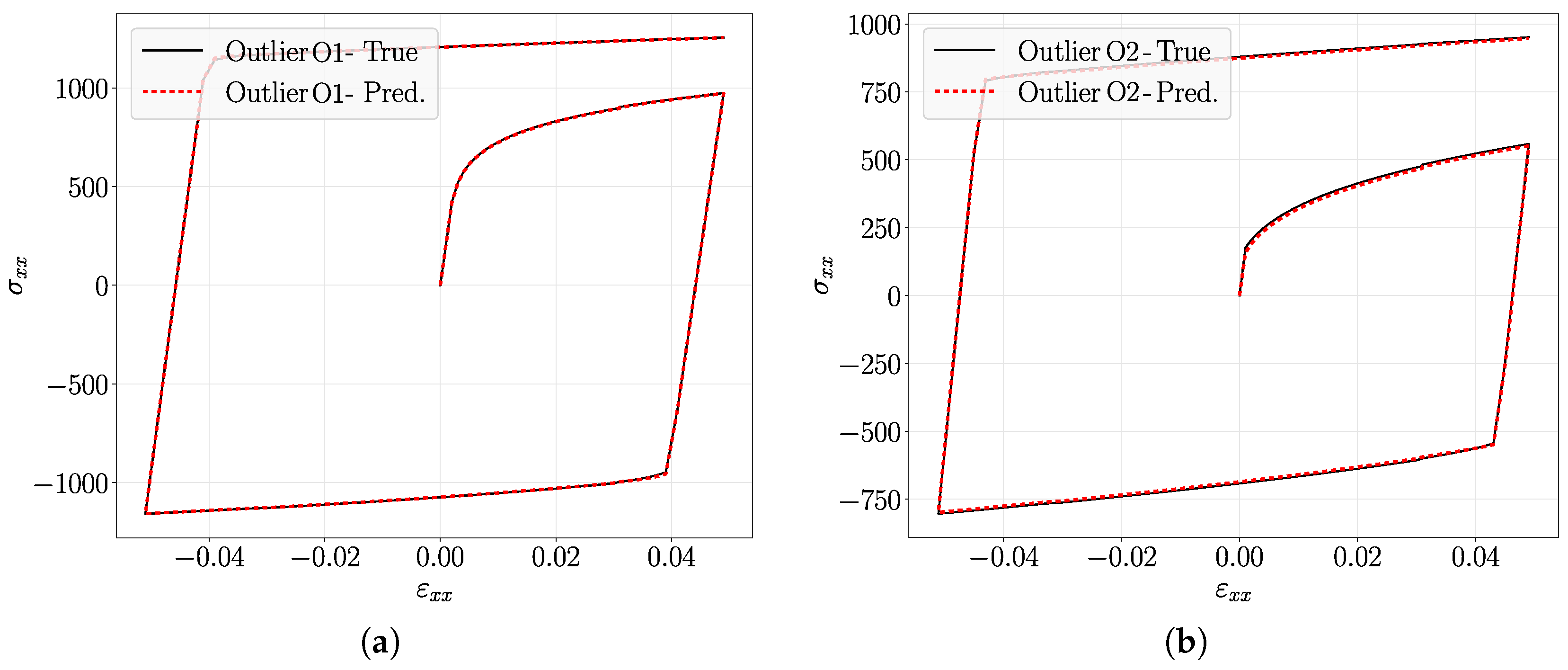
To further examine the predictions identified as outliers, two representative cases, denoted as Outliers O1 and O2, also represented in Figure 15, are analyzed in detail. Their true and predicted constitutive parameters are presented in

Table 9. Expected and predicted parameters for Outliers O1 and O2, together with the corresponding range-normalized absolute errors, $E_{\mathrm{RN}}$.

Outlier		K [MPa]	${\mathit{\sigma }}_0$ [MPa]	n	C [MPa]	$\mathit{\gamma }$
O1	Expected	1575.83	467.03	0.16	4661.74	307.07
	Predicted	1581.88	461.20	0.16	4390.25	448.54
	$E_{\mathrm{RN}}$	0.50%	0.50%	0.00%	0.27%	28.31%
O2	Expected	1546.53	170.67	0.34	1858.03	216.74
	Predicted	1549.50	147.87	0.34	878.87	360.52
	$E_{\mathrm{RN}}$	0.25%	1.94%	0.00%	0.99%	28.77%

, together with the corresponding range-normalized absolute errors, $E_{\mathrm{RN}}$. Despite being classified as outliers based on their overall MSE, the isotropic hardening parameters exhibit relatively small $E_{\mathrm{RN}}$ values, remaining below 2% for both cases. In contrast, the largest discrepancies are observed for $\gamma$, with $E_{\mathrm{RN}}$ values of approximately 28%. These results further highlight the greater difficulty of predicting the kinematic hardening parameters, particularly $\gamma$, from the reverse bending response.

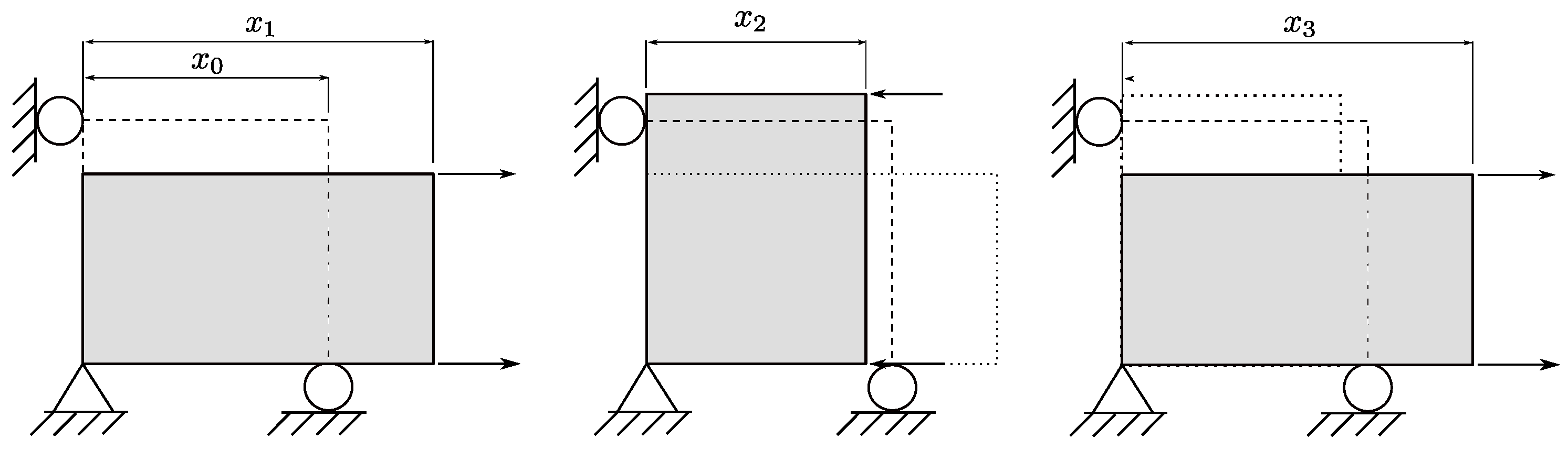
To evaluate the influence of the predicted constitutive parameters on the resulting material response, uniaxial tension–compression–tension (TCT) loading conditions were simulated using a single finite element model. This simplified numerical model provides a controlled framework to evaluate whether prediction errors in the constitutive parameters translate into significant differences in the corresponding stress–strain response. The model consists of a single S4R shell element with elastoplastic material behavior described by the combined isotropic–kinematic hardening model. A Young’s modulus of 210 GPa and an isotropic von Mises yield criterion were adopted throughout the analysis. As illustrated in Figure 16, the loading path comprises three consecutive stages: initial tension, reverse compression and subsequent tension. Prescribed displacements, denoted by $x_1$, $x_2$, and $x_3$, were applied to produce an equivalent plastic strain of approximately 0.05 during each loading stage. This strain level is representative of the plastic deformation experienced during the reverse bending test and therefore provides a suitable basis for evaluating the influence of parameter prediction errors on the constitutive response.

Figure 17 and Figure 18 compare the tension–compression–tension (TCT) stress–strain (${\sigma }_{xx}$–${\epsilon }_{xx}$) responses obtained using the true and predicted constitutive parameters for the representative cases Q2, Max, and Outliers O1 and O2, respectively. For each case, the target curve is generated using the true hardening parameters, while the predicted curve is obtained using the parameters identified by the Bi-LSTM model. The predicted and target stress–strain responses show close agreement for the five representative cases considered. Even for the Max case and the outliers, where the prediction errors in the kinematic hardening parameters are considerably larger, the resulting stress–strain curves remain similar. This indicates that relatively large errors in the individual values of C and $\gamma$ do not necessarily translate into significant differences in the overall constitutive response under the considered loading path.

4.2. Physically Constrained Loss Function

Although the proposed Bi-LSTM model provides highly accurate predictions for most cases, a small number of simulations produce physically inadmissible values for the kinematic hardening parameters C and $\gamma$. Since both parameters are required to remain non-negative to satisfy the constitutive formulation, these predictions represent a limitation of a purely data-driven regression model. Among the 5000 simulations, 12 cases yielded negative predictions for C and 16 for $\gamma$, whereas no negative values were obtained for the isotropic hardening parameters. These violations occur almost exclusively when the true parameter values are close to their lower bounds ($C=1000$ MPa and $\gamma =0$), where the prediction problem is more challenging.

A straightforward solution would be to employ a ReLU activation function in the output layer, thereby enforcing non-negative predictions. However, this approach is not suitable for the present framework because all target variables were normalized to the interval $[-1,1]$. Applying ReLU would truncate the normalized output space and invalidate the subsequent denormalization procedure. Even if the outputs were normalized to $[0,1]$, constraining the network through the activation function would unnecessarily restrict its extrapolation capability. While $\gamma$ is physically bounded by zero, the remaining parameters may assume values outside the sampled range while still remaining physically meaningful. Consequently, enforcing non-negativity through the activation function would introduce an undesirable architectural constraint rather than incorporating the underlying physical knowledge.

Instead of modifying the network architecture, physical admissibility was incorporated directly into the optimization process through a physically constrained loss function. This approach preserves the flexibility of the regression model while discouraging predictions that violate the constitutive constraints. In this context, a custom loss function is defined as the weighted combination of a standard regression term (mean squared error between predicted and true normalized values) and a penalty term associated with physical violations:

$${\mathcal{L}}_{\mathrm{total}}=(1-\lambda )·\mathrm{MSE}+\lambda ·{\mathrm{Penalty}}_{\mathrm{physical}},$$

(6)

where the scalar parameter $\lambda \in [0,1]$ controls the trade-off between data fidelity and physical admissibility. Since the network outputs are normalized to the interval $[-1,1]$, the predicted values used in the physically constrained penalty are first denormalized to their physical units. The penalty term is therefore applied to the physical predictions $\widehat{C}$ and $\widehat{\gamma }$ and is defined as:

$${\mathrm{Penalty}}_{\mathrm{physical}}={\displaystyle \frac{\mathrm{ReLU}(-\widehat{C})}{C_{\max }-C_{\min }}}+{\displaystyle \frac{\mathrm{ReLU}(-\widehat{\gamma })}{{\gamma }_{\max }-{\gamma }_{\min }}},$$

(7)

where the ReLU (Rectified Linear Unit) operator ensures that only negative values are penalized, while normalization by the parameter ranges prevents any single term from dominating the loss due to scale differences. The physical admissibility penalty therefore acts as a soft constraint, discouraging negative predictions without strictly enforcing their non-negativity.

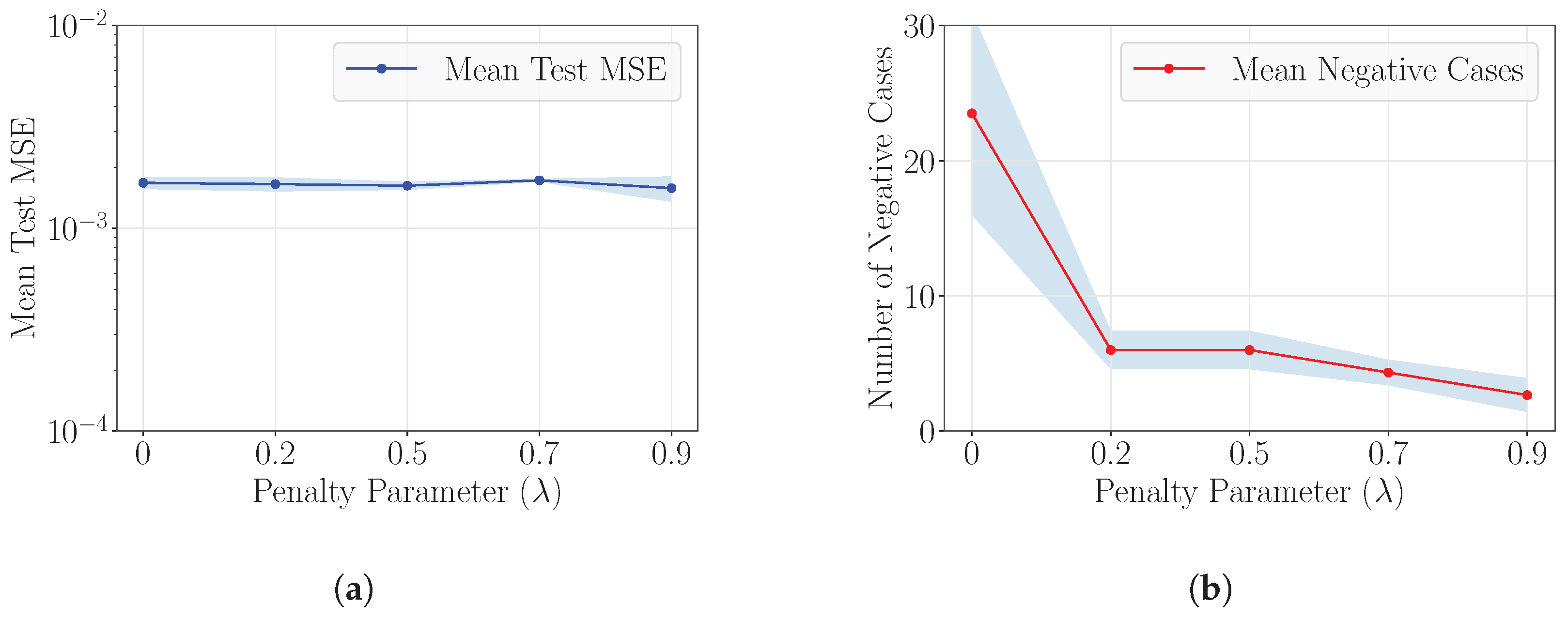
Figure 19 shows the impact of the penalty weight $\lambda$ in the physically constrained loss function on both prediction accuracy and physical admissibility. To account for the variability associated with network training, five independent training runs were performed for each value of $\lambda$. Figure 19a shows the variation in the mean test MSE with increasing values of $\lambda$, while Figure 19b shows the corresponding evolution of the mean number of predicted negative values for the kinematic parameters C and $\gamma$. As seen, the inclusion of the physical admissibility penalty has reduced effect on the prediction accuracy, as the MSE remains within the same order of magnitude across the investigated values of $\lambda$, with only minor variations. This indicates that incorporating physical constraints into the loss function does not compromise the model’s ability to fit the data. However, the number of negative cases is substantially reduced as $\lambda$ increases, dropping from more than 20 cases when $\lambda =0$ (i.e., no physical penalization) to fewer than 5 cases for $\lambda \ge 0.5$. This result shows the effectiveness of the penalty term in promoting physically admissible predictions. The diminishing marginal effect beyond $\lambda =0.2$ indicates that most of the reduction in physically inadmissible predictions is achieved at relatively low penalty weights. The value $\lambda =0.9$ was selected as the final penalty weight because it resulted in the largest number of physically admissible predictions among the investigated values of $\lambda$, while maintaining comparable prediction accuracy, as indicated by the test MSE. These results indicate that the physically constrained loss can substantially reduce physically inadmissible predictions while maintaining comparable prediction accuracy. The selected penalty weight therefore provides a practical balance between regression accuracy and physical admissibility.

Table 10. Expected and predicted material parameters for outliers O3, O4 and O5 using the unconstrained ($\lambda =0$) and physically constrained ($\lambda =0.9$) models, together with the corresponding range-normalized absolute errors, $E_{\mathrm{RN}}$.

Outlier		K [MPa]	${\mathit{\sigma }}_0$ [MPa]	n	C [MPa]	$\mathit{\gamma }$
O3	Expected	1211.82	747.36	0.10	1120.85	145.63
	Pred. ($\lambda =0$)	1214.34	746.12	0.10	$-1087.02$	291.34
	$E_{\mathrm{RN}}$	0.21%	0.11%	0.00%	2.23%	29.16%
	Pred. ($\lambda =0.9$)	1219.32	753.57	0.10	2710.83	286.16
	$E_{\mathrm{RN}}$	0.63%	0.53%	0.00%	1.61%	28.12%
O4	Expected	1479.00	369.71	0.29	4601.32	10.86
	Pred. ($\lambda =0$)	1475.50	367.08	0.29	5114.64	$-9.56$
	$E_{\mathrm{RN}}$	0.29%	0.22%	0.00%	0.52%	4.09%
	Pred. ($\lambda =0.9$)	1448.00	369.26	0.28	5831.57	11.11
	$E_{\mathrm{RN}}$	2.58%	0.04%	3.33%	1.24%	0.05%
O5	Expected	1061.38	587.72	0.10	2051.39	38.02
	Pred. ($\lambda =0$)	1075.61	584.87	0.10	$-1848.21$	$-23.23$
	$E_{\mathrm{RN}}$	1.19%	0.24%	0.00%	3.94%	12.26%
	Pred. ($\lambda =0.9$)	1062.71	590.00	0.10	$-85.68$	15.36
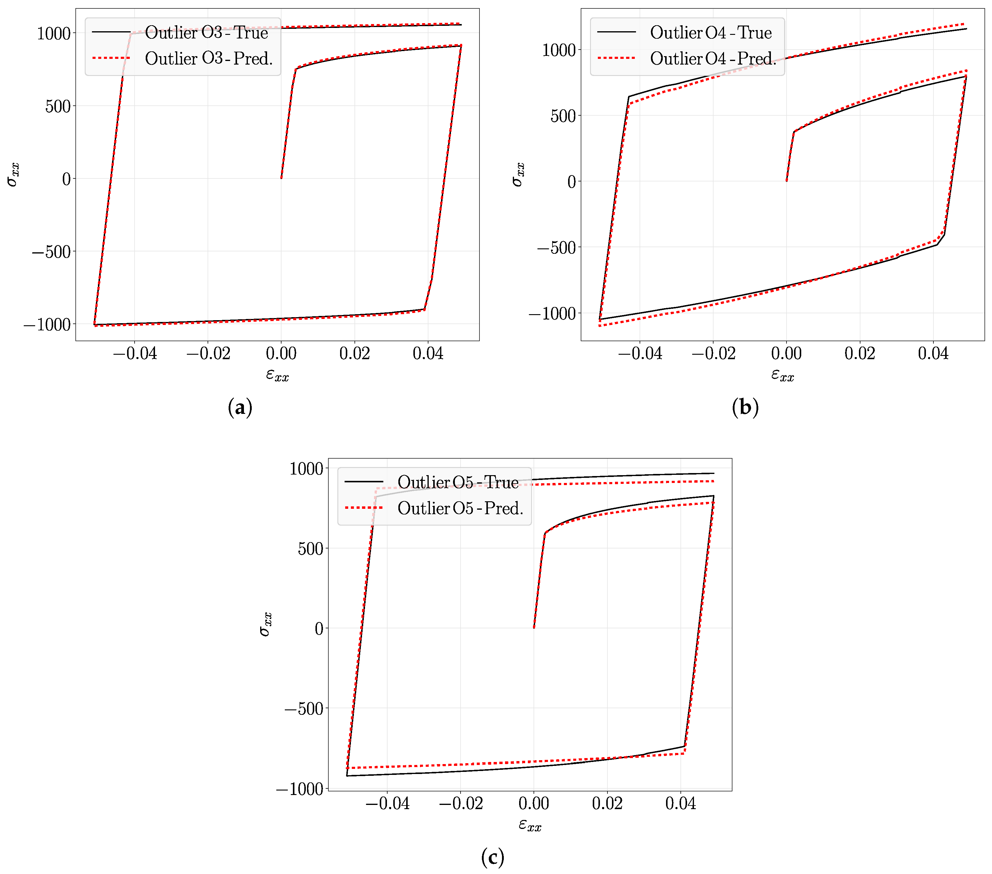
	$E_{\mathrm{RN}}$	0.11%	0.19%	0.00%	2.16%	4.53%

compares the expected and predicted material parameters for the representative outlier cases O3, O4 and O5. These cases were originally identified as producing negative predictions for the kinematic hardening parameters C or $\gamma$ when the standard loss function ($\lambda =0$) was used. The table compares the predictions obtained with the unconstrained model and with the best-performing physically constrained model ($\lambda =0.9$), which reduced the number of physically inadmissible predictions to only one case out of the 5000 simulations. For outliers O3 and O4, the physically constrained loss eliminated the negative predictions, yielding physically admissible values for all constitutive parameters. In contrast, outlier O5 still produced a slightly negative prediction for C, indicating that the proposed penalty considerably reduces, but does not completely eliminate, physically inadmissible solutions. This remaining inadmissible prediction highlights a limitation of the proposed soft constraint, which does not strictly guarantee physically admissible outputs. In such rare cases, the adopted post-processing strategy consists of setting any negative values of C or $\gamma$ to zero before using the predicted parameters in subsequent simulations. The corresponding $E_{\mathrm{RN}}$ values reported in Table 10 further illustrate the effect of enforcing physical admissibility on the prediction accuracy. For outlier O3, for example, the prediction of C changes from $-1087.02$ MPa for $\lambda =0$ to $2710.83$ MPa for $\lambda =0.9$. This correction not only yields a physically admissible value, but also reduces the $E_{\mathrm{RN}}$ from $2.23\%$ to $1.61\%$. Nevertheless, the predicted magnitude of C remains substantially higher than the expected value of 1120.85 MPa. This illustrates that enforcing physical admissibility can improve the normalized prediction error while still resulting in a considerable deviation in the absolute magnitude of a parameter. The magnitude of the improvement also varies between parameters. For example, a more pronounced reduction is observed for $\gamma$ in outlier O5, for which the $E_{\mathrm{RN}}$ decreases from 4.09% to 0.05%. The corresponding tension–compression–tension (TCT) responses are presented in Figure 20. Despite the corrections introduced by the physically constrained loss, the predicted constitutive parameters remain mechanically consistent and reproduce the overall material response even for these challenging edge cases.

Finally, a global assessment of the proposed framework is performed by evaluating the isotropic and kinematic hardening responses reconstructed from the predicted constitutive parameters over the complete dataset. While the previous sections analyzed representative prediction cases through tension–compression–tension simulations, the objective here is to quantify how the prediction errors propagate to the constitutive hardening laws themselves.

For the isotropic component, the evolution of the equivalent stress, $\sigma$, with the equivalent plastic strain, ${\epsilon }_p$, is described by the Swift hardening law, using both the predicted and true parameters:

$${\sigma }^{\mathrm{pred}}=\widehat{K}{\left({\left({\displaystyle \frac{{\widehat{\sigma }}_0}{\widehat{K}}}\right)}^{1/\widehat{n}}+{\epsilon }_p\right)}^{\widehat{n}},$$

(8)

$${\sigma }^{\mathrm{true}}=K{\left({\left({\displaystyle \frac{{\sigma }_0}{K}}\right)}^{1/n}+{\epsilon }_p\right)}^n,$$

(9)

where ${\sigma }^{\mathrm{pred}}$ and ${\sigma }^{\mathrm{true}}$ are the predicted and true equivalent stresses, respectively. The parameters $\widehat{K}$, ${\widehat{\sigma }}_0$ and $\widehat{n}$ represent the predicted isotropic hardening parameters, while K, ${\sigma }_0$ and n denote the corresponding true values. Similarly, for the kinematic component, the evolution of the backstress, $\alpha$, as a function of the equivalent plastic strain is evaluated using the Armstrong–Frederick hardening rule:

$${\alpha }^{\mathrm{pred}}={\displaystyle \frac{\widehat{C}}{\widehat{\gamma }}}·\left(1-e^{-\widehat{\gamma }{\epsilon }_p}\right),$$

(10)

$${\alpha }^{\mathrm{true}}={\displaystyle \frac{C}{\gamma }}·\left(1-e^{-\gamma {\epsilon }_p}\right),$$

(11)

where ${\alpha }^{\mathrm{pred}}$ and ${\alpha }^{\mathrm{true}}$ are the predicted and true backstress values, respectively. The parameters $\widehat{C}$ and $\widehat{\gamma }$ refer to the predicted kinematic hardening coefficients, C and $\gamma$ are the corresponding true values.

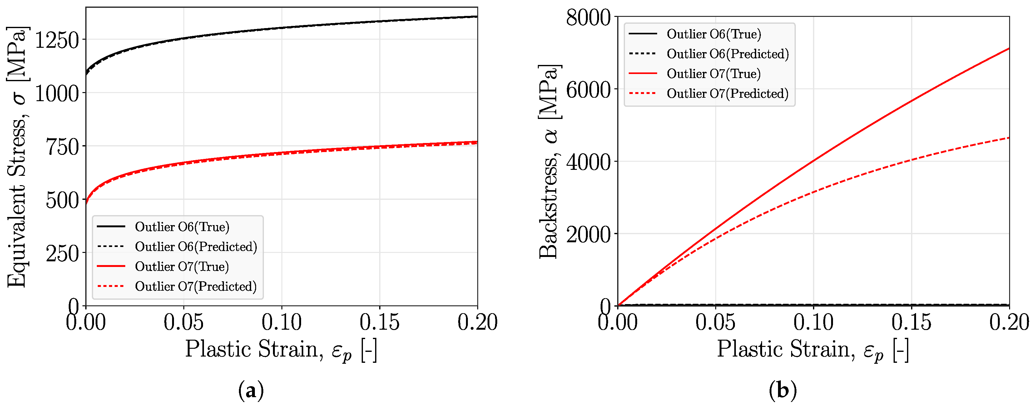
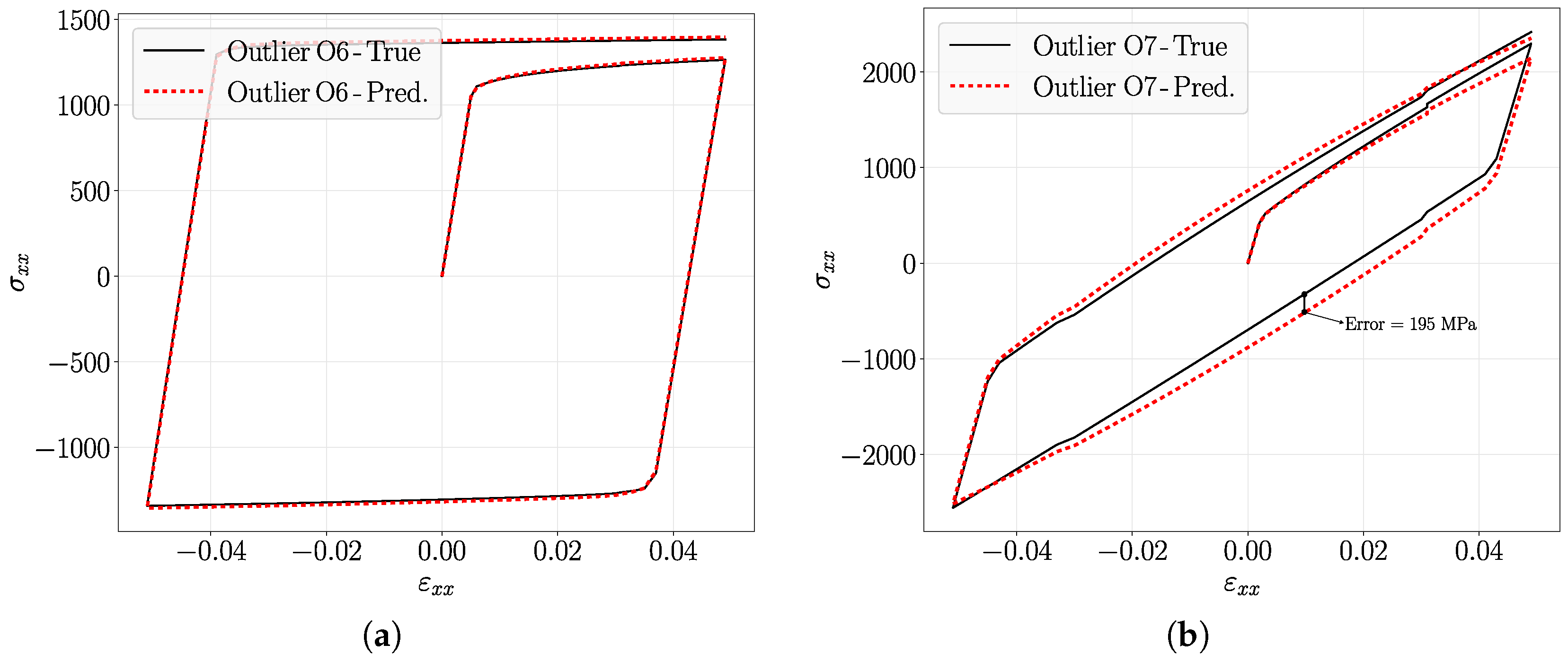
Two representative cases, Outliers O6 and O7, are selected to illustrate how differences between the predicted and target constitutive parameters propagate to the resulting material response. The corresponding material parameters are summarized in

Table 11. Expected and predicted parameters for Outliers O6 and O7, together with the corresponding range-normalized absolute errors, $E_{\mathrm{RN}}$.

Outlier		K [MPa]	${\mathit{\sigma }}_0$ [MPa]	n	C [MPa]	$\mathit{\gamma }$
O6	Expected	1492.19	1097.11	0.06	5253.91	291.02
	Predicted	1490.64	1083.54	0.06	12,158.02	369.35
	$E_{\mathrm{RN}}$	0.13%	1.16%	0.00%	6.98%	15.67%
O7	Expected	903.61	481.87	0.10	45,496.83	2.56
	Predicted	893.64	477.37	0.10	44,552.06	7.40
	$E_{\mathrm{RN}}$	0.83%	0.38%	0.00%	0.96%	0.97%

, while Figure 21 compares the reconstructed equivalent stress and backstress evolutions.

For both cases, the predicted equivalent stress curves show good agreement with the target responses, consistent with the small errors obtained for the isotropic hardening parameters. Outlier O6 is characterized by a large deviation in the predicted kinematic hardening modulus C, whereas Outlier O7 exhibits a substantially different predicted value of $\gamma$ from the target value. As indicated by the small errors in the isotropic hardening parameters, Figure 21a shows good agreement between the predicted and target equivalent stress curves for both cases. In contrast, the backstress evolution presented in Figure 21b shows more pronounced differences, particularly for O6, where the deviation in C affects the evolution of the backstress. For O7, the predicted and target backstress responses remain comparatively close over the considered plastic strain range, despite the difference between the predicted and target values of $\gamma$.

Figure 22 further illustrates how these differences affect the corresponding tension–compression–tension response. For Outlier O6, despite the comparatively large deviation in the predicted value of C, the reconstructed stress–strain curve remains very close to the target response, indicating a limited influence of this parameter deviation on the overall macroscopic response for this case. In contrast, Outlier O7 represents the most challenging case in terms of its effect on the reconstructed constitutive response. The difference between the predicted and target curves is more pronounced, with a maximum absolute stress difference of approximately 195 MPa, corresponding to about 55% of the target stress at the indicated point.

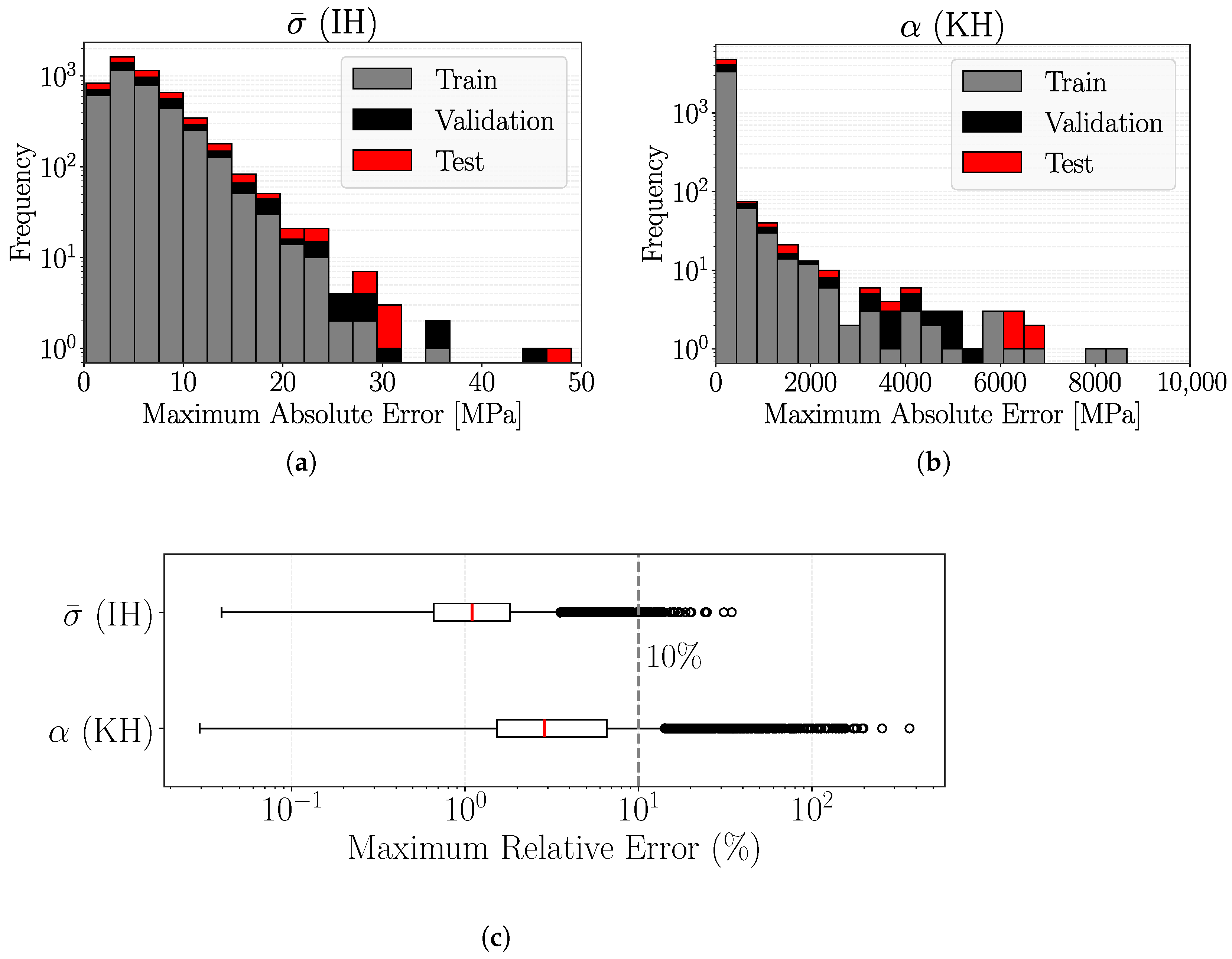
To quantify the overall effect of the prediction errors, the equivalent stress and backstress evolutions were reconstructed for all 5000 simulations using the predicted constitutive parameters over the equivalent plastic strain range ($0\le {\epsilon }_p\le 0.2$). Figure 23 summarizes the resulting maximum errors distributions. Most equivalent stress predictions exhibit maximum absolute errors below 20 MPa, corresponding to relative errors generally below 10%, with only a small number of isolated outliers exceeding 30 MPa. The backstress predictions present a broader error distribution, reflecting the greater difficulty of identifying the kinematic hardening parameters C and $\gamma$. The boxplot of the maximum relative errors further confirms this trend. The equivalent stress predictions remain tightly distributed, with the interquartile range below 10%, whereas the backstress errors are more dispersed, reflecting the larger variability in the prediction of the kinematic hardening parameters. The maximum absolute backstress errors reach approximately 10,000 MPa for a small number of isolated outlier cases. Although large absolute errors may occur for a limited number of outlier cases, the relative-error distribution shows that these cases are not representative of the overall behavior. The results therefore support the ability of the proposed framework to reconstruct the constitutive response for the large majority of the investigated material configurations.

4.3. Effect of Force-Measurement Noise on Parameter Prediction

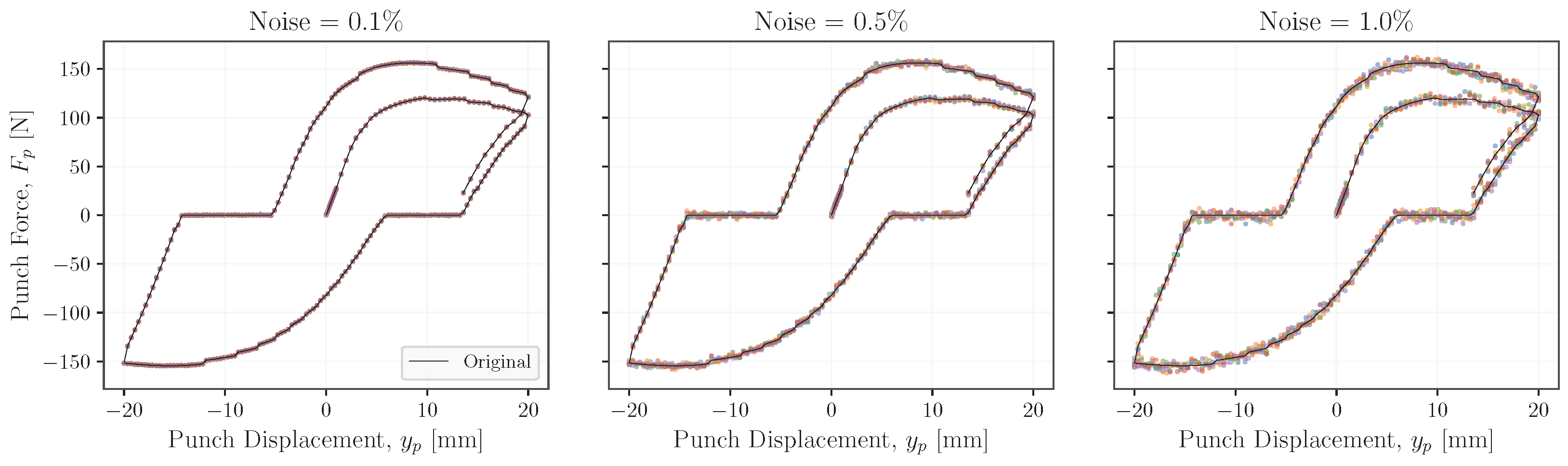
To evaluate the sensitivity of the trained Bi-LSTM model to measurement noise, a sensitivity analysis was performed by introducing controlled perturbations into the force signal of the test dataset (750 cases). Zero-mean Gaussian noise was added to the force measurements, while the displacement signal was kept unchanged. The noise level was defined as a percentage of the force range of each individual force–displacement curve, considering noise levels of 0.1%, 0.5%, and 1.0% to represent increasing levels of force-measurement uncertainty. For each noise level, 10 independent noise samples were generated for each test case to account for the stochastic nature of the measurement perturbation and to evaluate the variability of the resulting parameter predictions. The Bi-LSTM model was not retrained during this analysis.

Figure 24 shows the effect of the imposed force noise on a representative test curve. For each noise level, the original force–displacement response is shown together with five independent noise samples. As expected, the amplitude of the fluctuations increases progressively with the noise level. Nevertheless, the overall characteristics of the force–displacement response remain preserved.

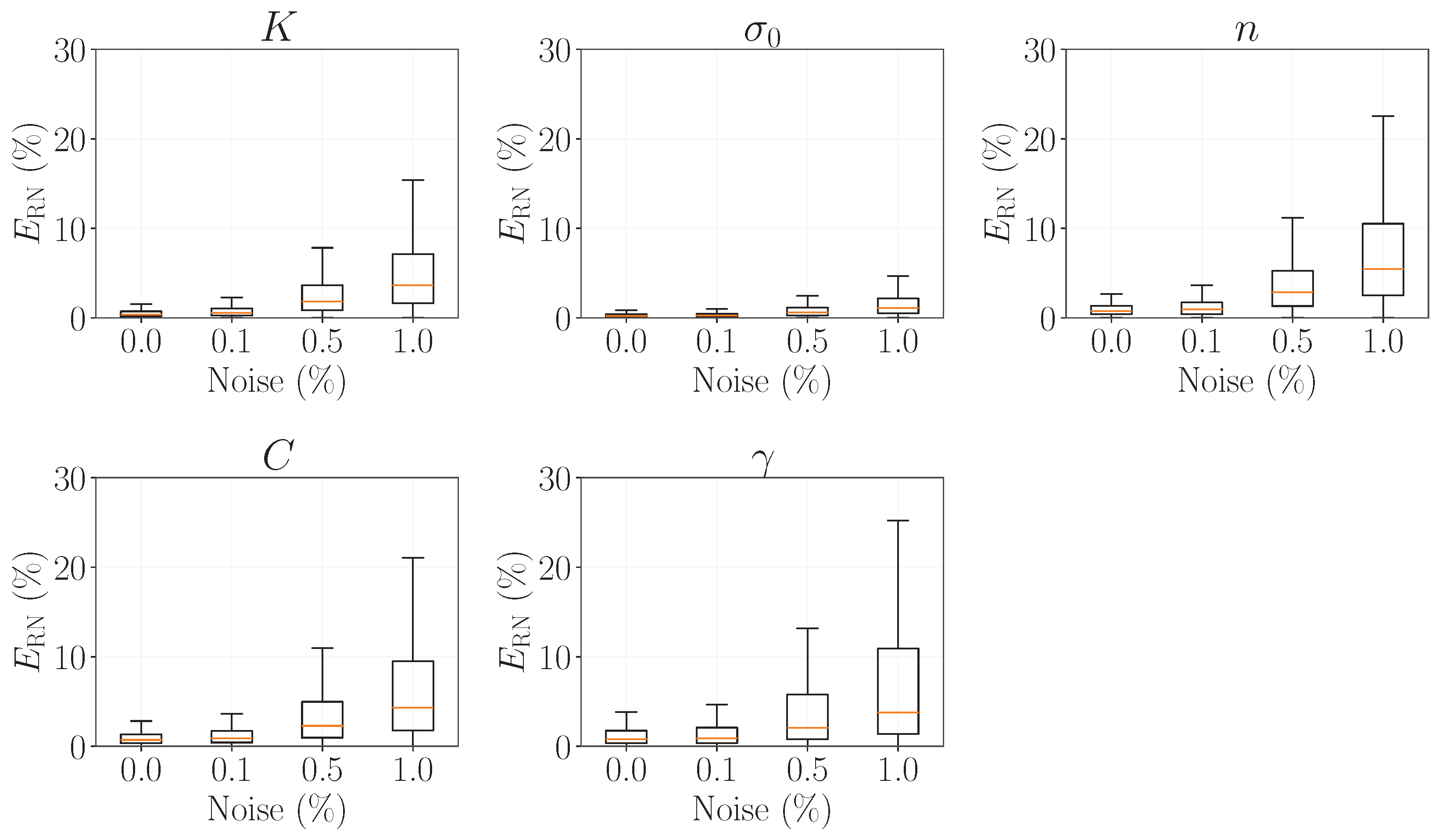
Figure 25 shows the distribution of the range-normalized absolute error, $E_{\mathrm{RN}}$ (Equation (5)), obtained for the five predicted constitutive parameters at each noise level. The results show that the influence of force noise is parameter-dependent. At low noise levels, the error distributions remain relatively concentrated, with only a limited change between 0.0% and 0.1% noise. For example, the median $E_{\mathrm{RN}}$ increases from 0.38% to 0.56% for K and from 0.22% to 0.25% for ${\sigma }_0$. As the noise level increases, a progressively larger increase in both the median error and the dispersion of the distributions is observed, particularly for n, C, and $\gamma$. At 1.0% noise, the median $E_{\mathrm{RN}}$ reaches 3.66% for K, 1.12% for ${\sigma }_0$, 5.45% for n, 4.34% for C, and 3.79% for $\gamma$, compared with 0.38%, 0.22%, 0.76%, 0.72%, and 0.79%, respectively, for the noise-free test data. Although the prediction error increases with noise, the median $E_{\mathrm{RN}}$ remains below 6% for all parameters even at the highest noise level considered.

The increase in the upper tail of the distributions is further characterized by the 95th percentile (P95), defined as the error below which 95% of the predictions fall. At 1.0% noise, the P95 reaches 16.90% for K, 5.45% for ${\sigma }_0$, 22.90% for n, 26.92% for C, and 37.12% for $\gamma$, compared with 1.82%, 0.89%, 2.80%, 4.10%, and 7.23%, respectively, for the noise-free test data. These results indicate that increasing force noise affects not only the median prediction error, but also the upper tail of the error distribution. The effect is particularly pronounced for the kinematic hardening parameters.

The corresponding quantitative metrics are summarized in

Table 12. Prediction errors obtained under different levels of force-measurement noise.

Noise (%)	Parameter	MAE	RMSE	NRMSE (%)
0.0%	K	7.14	11.15	0.93
	${\sigma }_0$	3.76	5.79	0.50
	n	0.003	0.004	1.45
	C	1188.97	2041.84	2.06
	$\gamma$	9.31	20.04	4.01
0.1%	K	9.96	14.99	1.25
	${\sigma }_0$	4.21	6.37	0.55
	n	0.004	0.006	1.84
	C	1459.58	2426.90	2.45
	$\gamma$	10.77	22.83	4.57
0.5%	K	33.32	48.90	4.08
	${\sigma }_0$	10.39	15.50	1.35
	n	0.012	0.017	5.73
	C	4141.24	7018.95	7.09
	$\gamma$	25.84	48.79	9.76
1.0%	K	65.18	94.49	7.87
	${\sigma }_0$	19.67	29.47	2.56
	n	0.023	0.033	10.91
	C	7672.22	12,588.89	12.72
	$\gamma$	45.31	80.12	16.02

, including the mean absolute error, root mean square error, and normalized root mean square error (Equation (4)). The results confirm the trends observed in the boxplots, with a progressive increase in prediction error as the noise level increases. The larger increase observed for n, C, and $\gamma$ is consistent with the broader error distributions shown in Figure 25. Overall, the results provide an indication of how measurement uncertainty in the force signal can propagate into the identified constitutive parameters. The relatively small changes observed at 0.1% noise suggest that small perturbations in the force signal have a limited effect on the parameter predictions. However, the substantially larger errors observed at 0.5% and 1.0% noise, particularly for n, C, and $\gamma$, indicate that the sensitivity of the inverse prediction increases as the quality of the force signal deteriorates. This behavior is particularly relevant for the application of the proposed approach to experimental bending tests, since the force signal used as input to the trained model is directly affected by experimental measurement uncertainty. It should be noted that the present analysis considers only perturbations in the force signal and therefore does not account for other sources of uncertainty that may arise in experimental testing.

4.4. Experimental Validation

The proposed framework was further evaluated using experimental reverse bending tests performed on two advanced high-strength steels, DP500 and DP780. Unlike the previous analyses, which relied exclusively on synthetic data, this validation assesses the ability of the trained network to identify constitutive parameters directly from experimental force–displacement curves of DP500 and DP780, which were not included in the synthetic dataset used for model development.

Table 13. Comparison of the IKH parameters identified using the proposed reverse bending (Bi-LSTM) methodology and the tension–compression methodology based on genetic algorithm (GA) optimization for DP500 and DP780 steels.

Material	Identification Method	K [MPa]	${\mathit{\sigma }}_0$ [MPa]	n	C [MPa]	$\mathit{\gamma }$
DP500	Reverse Bending (Bi-LSTM)	616.08	243.3	0.21	67,824	374.8
	Tension–Compression (GA)	632.6	273.8	0.334	27,710	124.2
DP780	Reverse Bending (Bi-LSTM)	647.1	326.1	0.27	69,941	206.1
	Tension–Compression (GA)	651.8	373.2	0.191	38,850	88.3

compares the constitutive parameters predicted by the proposed Bi-LSTM framework from the reverse bending experiments with those previously identified in Section 2.2 using a conventional inverse identification procedure based on tension–compression tests. Although noticeable differences are observed between the identified parameter sets, these differences cannot be interpreted as evidence that either identification is inaccurate, since the two parameter sets were obtained from different experimental responses and identification procedures.

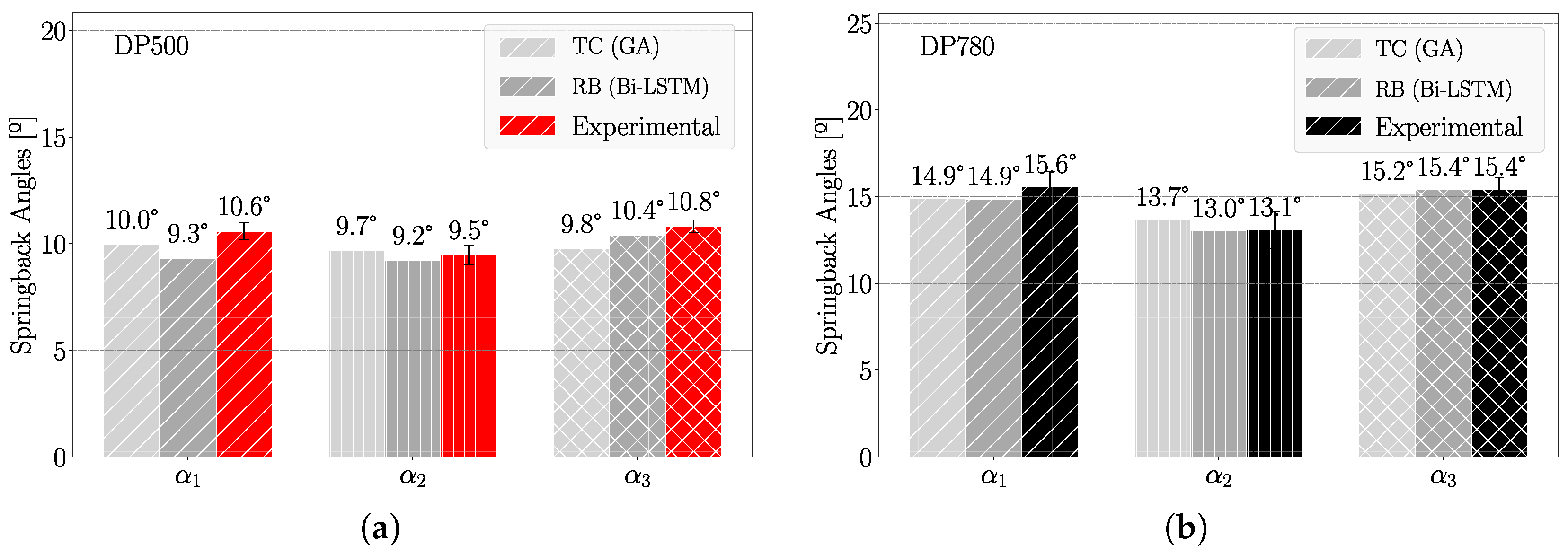
To evaluate the practical significance of these differences, both parameter sets were used in the finite element model of the reverse bending test presented in Section 2.3.2. The predicted springback angles, ${\alpha }_1$, ${\alpha }_2$, and ${\alpha }_3$, defined in Figure 4 and measured after unloading at each of the three bending stages, were then compared with the corresponding experimental measurements. Figure 26 presents the experimental springback angles together with the finite element predictions obtained using the constitutive parameters identified from the reverse bending (Bi-LSTM) and tension–compression (GA) methodologies for the DP500 and DP780 steels. For both materials, the finite element simulations based on the Bi-LSTM predictions show good agreement with the experimentally measured springback angles.

It should be noted, however, that the three springback angles measured after the successive loading stages provide a limited number of scalar observables compared with the five constitutive parameters being identified. Therefore, agreement with the experimental springback response does not establish the uniqueness of the identified parameter set or the accuracy of the individual constitutive parameters. Since the experimental assessment was performed using the same reverse bending configuration considered in the development of the FE framework, an additional validation using an independent loading configuration, would provide stronger evidence of the transferability of the proposed approach.

5. Conclusions

This work presented a machine learning framework for the identification of combined isotropic–kinematic hardening parameters from a reverse bending test. The proposed methodology combines finite element simulations, synthetic dataset generation and a bidirectional long short-term memory (Bi-LSTM) network to directly predict the constitutive parameters from force–displacement curves, eliminating the iterative optimization procedures typically required by finite element model updating approaches.

A synthetic dataset comprising 5000 finite element simulations was generated using Sobol sampling and employed to train the proposed network. The resulting Bi-LSTM model achieved coefficients of determination ($R^2$) values above 0.99 for the isotropic hardening parameters (K, ${\sigma }_0$ and n) and approximately 0.98–0.99 for the kinematic parameters (C and $\gamma$). The range-normalized error analysis showed errors below 10% for K and ${\sigma }_0$, while slightly larger maximum errors were observed for n (13.83%), C (15.27%), and particularly $\gamma$ (37.36%), which exhibited the largest variability in prediction error.

A physically constrained loss function was introduced to penalize negative predictions of the kinematic hardening parameters. This modification reduced the number of physically inadmissible predictions from approximately 30 cases to a single case out of the 5000 simulations, while maintaining essentially unchanged prediction accuracy. However, since the constraint is implemented as a soft penalty, it does not strictly guarantee physically admissible predictions in all cases. The reconstructed constitutive responses showed that relatively large errors in the predicted kinematic parameters were concentrated in the identified outlier cases, while most of the investigated cases showed limited changes in the stress–strain response.

The force-measurement noise analysis showed that increasing noise levels progressively increase both the typical prediction error and the dispersion of the parameter predictions. The effect was particularly pronounced for n, C, and $\gamma$. In contrast, ${\sigma }_0$ exhibited the lowest sensitivity to force noise, with an NRMSE of only 2.56% at the highest noise level considered.

Finally, the proposed framework was evaluated experimentally using reverse bending tests on DP500 and DP780 steels. The parameter sets predicted by the Bi-LSTM yielded finite element predictions in good agreement with the experimentally measured springback angles. Since the experimental parameter sets obtained from reverse bending and tension–compression were derived independently from different experimental responses and identification procedures, their differences cannot be interpreted as direct evidence of parameter accuracy or non-uniqueness.

Although the trained model enables near-instantaneous parameter prediction, the proposed approach has limitations when applied beyond the conditions represented in the training dataset. Substantially different materials, sheet thicknesses, geometries, or loading conditions may require additional training data and model retraining. Optimization-based identification approaches, although requiring a new iterative procedure for each identification, offer greater flexibility to address changes in material and experimental conditions. Transfer learning [59] techniques may allow the trained model to be extended to new but related conditions using a smaller amount of additional training data and without requiring complete retraining.

To further improve the predictive capability of the proposed framework, additional training data should be incorporated, particularly in regions of the parameter space where the largest prediction errors occur. A more targeted sampling strategy in these critical regions could improve model accuracy. Another potential improvement is refining the discretization of the force–displacement curves. In the present work, each curve was resampled to 300 points to balance computational efficiency and representativeness. A finer discretization may capture more subtle variations in the material response, potentially improving the prediction of the constitutive parameters. In addition to the global force–displacement response, richer input features could be incorporated into the machine learning model. For example, the evolution of the strain distribution through the sheet thickness during reverse bending would provide additional information for characterizing kinematic hardening. Although such data can be readily extracted from finite element simulations, their experimental measurement remains challenging, particularly for thin sheets. Derived quantities, such as the cumulative force–displacement area, which is directly related to the energy dissipated during deformation, also represent promising input features.

A formal identifiability analysis would also be valuable to assess the uniqueness and sensitivity of the constitutive parameters and to quantify the extent to which different parameter combinations may produce similar responses. Finally, validation under an independent loading configuration, such as the U-shaped channel geometry of the Numisheet Benchmark [60], would provide stronger evidence of the transferability of the proposed framework beyond the reverse bending configuration considered in the present study. Finally, a systematic comparison with alternative machine-learning architectures, such as MLP, LSTM, GRU and 1D-CNN models, could provide further insight into the relative advantages of the Bi-LSTM architecture and represents a relevant direction for future work.

References

1. Taylor, G.I.; Elam, C.F. Bakerian Lecture. The distortion of an aluminium crystal during a tensile test. Proc. R. Soc. Lond. Ser. A Contain. Pap. Math. Phys. Character 1923, 102, 643–667. [Google Scholar] [CrossRef] [Scilit]
2. Schmid, E.; Boas, W.; Rawlins, F.I.G. Kristallplastizität. J. Phys. Chem. 1934, 39, 1248. [Google Scholar] [CrossRef] [Scilit]
3. Roters, F.; Eisenlohr, P.; Hantcherli, L.; Tjahjanto, D.D.; Bieler, T.R.; Raabe, D. Overview of constitutive laws, kinematics, homogenization and multiscale methods in crystal plasticity finite-element modeling: Theory, experiments, applications. Acta Mater. 2010, 58, 1152–1211. [Google Scholar] [CrossRef] [Scilit]
4. Grilo, T.J. Development of Computational Anisotropic Hypoelastic- and Hyperelastic-Based Models Including Nonlinear Kinematic Hardening. Ph.D. Thesis, Universidade de Aveiro Departamento de Engenharia Mecanica, Aveiro, Portugal, 2015. [Google Scholar]
5. Mendiguren, J.; Trujillo, J.J.; Cortés, F.; Galdos, L. An extended elastic law to represent non-linear elastic behaviour: Application in computational metal forming. Int. J. Mech. Sci. 2013, 77, 57–64. [Google Scholar] [CrossRef] [Scilit]
6. Yoshida, F.; Uemori, T. A model of large-strain cyclic plasticity and its application to springback simulation. Int. J. Mech. Sci. 2008, 50, 428–439. [Google Scholar]
7. Barlat, F.; Brem, J.; Yoon, J.; Chung, K.; Dick, R.; Lege, D.; Pourboghrat, F.; Choi, S.H.; Chu, E. Plane stress yield function for aluminum alloy sheets—part 1: Theory. Int. J. Plast. 2003, 19, 1297–1319. [Google Scholar] [CrossRef] [Scilit]
8. Cazacu, O.; Plunkett, B.; Barlat, F. Orthotropic yield criterion for hexagonal closed packed metals. Int. J. Plast. 2006, 22, 1171–1194. [Google Scholar] [CrossRef] [Scilit]
9. Yang, H.; Zhang, W.; Zhuang, X.; Zhao, Z. Phenomenological Modeling of Deformation-Induced Anisotropic Hardening Behaviors: A Review. Metals 2023, 13, 364. [Google Scholar] [CrossRef] [Scilit]
10. Barlat, F.; Gracio, J.J.; Lee, M.G.; Rauch, E.F.; Vincze, G. An alternative to kinematic hardening in classical plasticity. Int. J. Plast. 2011, 27, 1309–1327. [Google Scholar] [CrossRef] [Scilit]
11. Lee, M.G.; Kim, D.; Kim, C.; Wenner, M.L.; Chung, K. Spring-back evaluation of automotive sheets based on isotropic–kinematic hardening laws and non-quadratic anisotropic yield functions, part III: Applications. Int. J. Plast. 2005, 21, 915–953. [Google Scholar] [CrossRef] [Scilit]
12. Versino, D.; Tonda, A.; Bronkhorst, C.A. Data driven modeling of plastic deformation. Comput. Methods Appl. Mech. Eng. 2017, 318, 981–1004. [Google Scholar] [CrossRef] [Scilit]
13. Prates, P.A.; Pereira, A.F.G.; Sakharova, N.A.; Oliveira, M.C.; Fernandes, J.V. Inverse strategies for identifying the parameters of constitutive laws of metal sheets. Adv. Mater. Sci. Eng. 2016, 2016, 4152963. [Google Scholar] [CrossRef] [Scilit]
14. Latourte, F.; Chrysochoos, A.; Pagano, S.; Wattrisse, B. Elastoplastic behavior identification for heterogeneous loadings and materials. Exp. Mech. 2007, 48, 435–449. [Google Scholar] [CrossRef] [Scilit]
15. Fu, J.; Barlat, F.; Kim, J.H.; Pierron, F. Application of the virtual fields method to the identification of the homogeneous anisotropic hardening parameters for advanced high strength steels. Int. J. Plast. 2017, 93, 229–250. [Google Scholar] [CrossRef] [Scilit]
16. Périé, J.N.; Leclerc, H.; Roux, S.; Hild, F. Digital image correlation and biaxial test on composite material for anisotropic damage law identification. Int. J. Solids Struct. 2009, 46, 2388–2396. [Google Scholar] [CrossRef] [Scilit]
17. Chaparro, B.M.; Thuillier, S.; Menezes, L.F.; Manach, P.Y.; Fernandes, J.V. Material parameters identification: Gradient-based, genetic and hybrid optimization algorithms. Comput. Mater. Sci. 2008, 44, 339–346. [Google Scholar] [CrossRef] [Scilit]
18. Aguir, H.; BelHadjSalah, H.; Hambli, R. Parameter identification of an elasto-plastic behaviour using artificial neural networks–genetic algorithm method. Mater. Des. 2011, 32, 48–53. [Google Scholar] [CrossRef] [Scilit]
19. Abbassi, F.; Belhadj, T.; Mistou, S.; Zghal, A. Parameter identification of a mechanical ductile damage using artificial neural networks in sheet metal forming. Mater. Des. 2013, 45, 605–615. [Google Scholar] [CrossRef] [Scilit]
20. Schulte, R.; Karca, C.; Ostwald, R.; Menzel, A. Machine learning-assisted parameter identification for constitutive models based on concatenated loading path sequences. Eur. J. Mech.-A/Solids 2023, 98, 104854. [Google Scholar] [CrossRef] [Scilit]
21. Marques, A.; Pereira, A.; Ribeiro, B.; Prates, P.A. On the identification of material constitutive model parameters using machine learning algorithms. Key Eng. Mater. 2022, 926, 2146–2153. [Google Scholar] [CrossRef] [Scilit]
22. Huber, N.; Tsakmakis, C. A neural network tool for identifying the material parameters of a finite deformation viscoplasticity model with static recovery. Comput. Methods Appl. Mech. Eng. 2001, 191, 353–384. [Google Scholar] [CrossRef] [Scilit]
23. Ktari, Z.; Leitão, C.; Prates, P.A.; Khalfallah, A. Mechanical design of ring tensile specimen via surrogate modelling for inverse material parameter identification. Mech. Mater. 2021, 153, 103673. [Google Scholar] [CrossRef] [Scilit]
24. Bouchard, P.O.; Bourgeon, L.; Fayolle, S.; Mocellin, K. An enhanced Lemaitre model formulation for materials processing damage computation. Int. J. Mater. Form. 2010, 4, 299–315. [Google Scholar] [CrossRef] [Scilit]
25. Yao, D.; Duan, Y.C.; Li, M.Y.; Guan, Y.P. Hybrid identification method of coupled viscoplastic-damage constitutive parameters based on BP neural network and genetic algorithm. Eng. Fract. Mech. 2021, 257, 108027. [Google Scholar] [CrossRef] [Scilit]
26. Huang, C.; El Hami, A.; Radi, B. Metamodel-based inverse method for parameter identification: Elastic–plastic damage model. Eng. Optim. 2016, 49, 633–653. [Google Scholar] [CrossRef] [Scilit]
27. Bastos, N.; Prates, P.A.; Andrade-Campos, A. Material parameter identification of elastoplastic constitutive models using machine learning approaches. Key Eng. Mater. 2022, 926, 2193–2200. [Google Scholar] [CrossRef] [Scilit]
28. Marques, A.E.; Parreira, T.G.; Pereira, A.F.G.; Ribeiro, B.M.; Prates, P.A. Machine learning application to the identification of sheet metal constitutive model parameters. Mach. Learn. Comput. Sci. Eng. 2025, 1, 10. [Google Scholar] [CrossRef] [Scilit]
29. Tariq, A.; Deliktaş, B. An Inverse Parameter Identification in Finite Element Problems Using Machine Learning-Aided Optimization Framework. Exp. Mech. 2025, 65, 325–349. [Google Scholar] [CrossRef] [Scilit]
30. Mitreiro, D.; Prates, P.A.; Andrade-Campos, A. Reducing mesh dependency in dataset generation for machine learning prediction of constitutive parameters in sheet metal forming. Metals 2025, 15, 534. [Google Scholar] [CrossRef] [Scilit]
31. Morand, L.; Helm, D. A mixture of experts approach to handle ambiguities in parameter identification problems in material modeling. Comput. Mater. Sci. 2019, 167, 85–91. [Google Scholar] [CrossRef] [Scilit]
32. Guo, Z.; Bai, R.; Lei, Z.; Jiang, H.; Liu, D.; Zou, J.; Yan, C. CPINet: Parameter identification of path-dependent constitutive model with automatic denoising based on CNN–LSTM. Eur. J. Mech.-A/Solids 2021, 90, 104327. [Google Scholar] [CrossRef] [Scilit]
33. Cruz, D.J.; Barbosa, M.R.; Santos, A.D.; Amaral, R.L.; de Sá, J.C.; Fernandes, J.V. Recurrent neural networks and three-point bending test on the identification of material hardening parameters. Metals 2024, 14, 84. [Google Scholar] [CrossRef] [Scilit]
34. Ghaboussi, J.; Sidarta, D. New nested adaptive neural networks (NANN) for constitutive modeling. Comput. Geotech. 1998, 22, 29–52. [Google Scholar] [CrossRef] [Scilit]
35. Abueidda, D.W.; Koric, S.; Sobh, N.A.; Sehitoglu, H. Deep learning for plasticity and thermo-viscoplasticity. Int. J. Plast. 2021, 136, 102852. [Google Scholar] [CrossRef] [Scilit]
36. Ghavamian, F.; Simone, A. Accelerating multiscale finite element simulations of history-dependent materials using a recurrent neural network. Comput. Methods Appl. Mech. Eng. 2019, 357, 112594. [Google Scholar] [CrossRef] [Scilit]
37. Gorji, M.B.; Mozaffar, M.; Heidenreich, J.N.; Cao, J.; Mohr, D. On the potential of recurrent neural networks for modeling path dependent plasticity. J. Mech. Phys. Solids 2020, 143, 103972. [Google Scholar] [CrossRef] [Scilit]
38. Mozaffar, M.; Bostanabad, R.; Chen, W.; Ehmann, K.; Cao, J.; Bessa, M.A. Deep learning predicts path-dependent plasticity. Proc. Natl. Acad. Sci. USA 2019, 116, 26414–26420. [Google Scholar] [CrossRef] [Scilit] [PubMed]
39. Bonatti, C.; Mohr, D. On the importance of self-consistency in recurrent neural network models representing elasto-plastic solids. J. Mech. Phys. Solids 2022, 158, 104697. [Google Scholar] [CrossRef] [Scilit]
40. Huber, N.; Tsakmakis, C. Determination of constitutive properties from spherical indentation data using neural networks. Part i: The case of pure kinematic hardening in plasticity laws. J. Mech. Phys. Solids 1999, 47, 1569–1588. [Google Scholar] [CrossRef] [Scilit]
41. Huber, N.; Tsakmakis, C. Determination of constitutive properties from spherical indentation data using neural networks. Part ii: Plasticity with nonlinear isotropic and kinematichardening. J. Mech. Phys. Solids 1999, 47, 1589–1607. [Google Scholar] [CrossRef] [Scilit]
42. Swift, H. Plastic instability under plane stress. J. Mech. Phys. Solids 1952, 1, 1–18. [Google Scholar] [CrossRef] [Scilit]
43. Armstrong, P.J.; Frederick, C.O. A Mathematical Representation of the Multiaxial Bauschinger Effect; Berkeley Nuclear Laboratories: Berkeley, CA, USA, 1966; Volume 731. [Google Scholar]
44. Prager, W. A New Method of Analyzing Stresses and Strains in Work-Hardening Plastic Solids. J. Appl. Mech. 1956, 23, 493–496. [Google Scholar] [CrossRef] [Scilit]
45. Amaral, R.R.L. Development of Accurate Numerical Methodologies Applied to the Stamping of Advanced High Strength Steels and Experimental Validation. Ph.D. Thesis, University of Porto, Porto, Portugal, 2020. [Google Scholar] [CrossRef]
46. ASTM E8/E8M-16ae1; Standard Test Methods for Tension Testing of Metallic Materials. American Society for Testing and Materials: West Conshohocken, PA, USA, 2016.
47. Cruz, D.J.; Xavier, J.; Amaral, R.L.; Santos, A.D. A Miniaturized Device Coupled with Digital Image Correlation for Mechanical Testing. Micromachines 2022, 13, 2027. [Google Scholar] [CrossRef] [Scilit] [PubMed]
48. Gu, B.; He, J.; Li, S.; Chen, Y.; Li, Y. Cyclic Sheet Metal Test Comparison and Parameter Calibration for Springback Prediction of Dual-Phase Steel Sheets. J. Manuf. Sci. Eng. 2017, 139. [Google Scholar] [CrossRef] [Scilit]
49. Ghaei, A.; Green, D.E.; Thuillier, S.; Morestin, F. On the use of cyclic shear, bending and uniaxial tension–compression tests to reproduce the cyclic response of sheet metals. Proc. Inst. Mech. Eng. Part B J. Eng. Manuf. 2014, 229, 453–462. [Google Scholar] [CrossRef] [Scilit]
50. Yoshida, F.; Urabe, M.; Toropov, V. Identification of material parameters in constitutive model for sheet metals from cyclic bending tests. Int. J. Mech. Sci. 1998, 40, 237–249. [Google Scholar] [CrossRef] [Scilit]
51. Geng, L.; Shen, Y.; Wagoner, R. Anisotropic hardening equations derived from reverse-bend testing. Int. J. Plast. 2002, 18, 743–767. [Google Scholar] [CrossRef] [Scilit]
52. Omerspahic, E.; Mattiasson, K.; Enquist, B. Identification of material hardening parameters by three-point bending of metal sheets. Int. J. Mech. Sci. 2006, 48, 1525–1532. [Google Scholar] [CrossRef] [Scilit]
53. Zang, S.l.; Lee, M.G.; Sun, L.; Kim, J.H. Measurement of the Bauschinger behavior of sheet metals by three-point bending springback test with pre-strained strips. Int. J. Plast. 2014, 59, 84–107. [Google Scholar] [CrossRef] [Scilit]
54. Zhao, K.M.; Lee, J.K. Finite element analysis of the three-point bending of sheet metals. J. Mater. Process. Technol. 2002, 122, 6–11. [Google Scholar] [CrossRef] [Scilit]
55. Silvestre, E.; Mendiguren, J.; Galdos, L.; Sáenz de Argandoña, E. Comparison of the hardening behaviour of different steel families: From mild and stainless steel to advanced high strength steels. Int. J. Mech. Sci. 2015, 101–102, 10–20. [Google Scholar] [CrossRef] [Scilit]
56. Sobol’, I. On the distribution of points in a cube and the approximate evaluation of integrals. USSR Comput. Math. Math. Phys. 1967, 7, 86–112. [Google Scholar] [CrossRef] [Scilit]
57. Abadi, M.; Agarwal, A.; Barham, P.; Brevdo, E.; Chen, Z.; Citro, C.; Corrado, G.S.; Davis, A.; Dean, J.; Devin, M.; et al. TensorFlow: Large-Scale Machine Learning on Heterogeneous Systems. 2015. Available online: https://www.tensorflow.org/ (accessed on 20 June 2026).
58. Chollet, F. Keras. 2015. Available online: https://keras.io (accessed on 20 June 2026).
59. Heidenreich, J.N.; Bonatti, C.; Mohr, D. Transfer learning of recurrent neural network-based plasticity models. Int. J. Numer. Methods Eng. 2023, 125, e7357. [Google Scholar] [CrossRef] [Scilit]
60. Oliveira, M.; Alves, J.; Chaparro, B.; Menezes, L. Study on the influence of work-hardening modeling in springback prediction. Int. J. Plast. 2007, 23, 516–543. [Google Scholar] [CrossRef] [Scilit]
Figure 1. Comparison of experimental stress–strain curves with calculated results using the IH and IKH models for (a) DP500 and (b) DP780 dual-phase steels.
Metals 16 01030 g001
Figure 2. Boundary conditions of (a) the full contact model based on Zhao and Lee [54] and (bd) equivalent non-contact models that preserve bending moments at Point A. Data from [54].
Metals 16 01030 g002
Figure 3. Representation of (a,b) the reverse bending setup and (c) the corresponding schematic illustrating the clamped end, roller spacing (b), loading distance (L) and applied force (F).
Metals 16 01030 g003
Figure 4. Reverse bending test: (a) first loading stage with displacement d 1 and springback angle α 1 ; (b) second loading stage with reverse displacement d 2 and springback angle α 2 ; and (c) third loading stage with displacement d 3 and springback angle α 3 .
Metals 16 01030 g004
Figure 5. Images captured during the reverse bending test for the DP500 material, at the end of (a,b) step 1, (c,d) step 2 and (e,f) step 3; the left images show the specimen before elastic recovery, while the right images show the specimen after elastic recovery.
Metals 16 01030 g005
Figure 6. Schematic representation of the finite element model used for the reverse bending test.
Metals 16 01030 g006
Figure 7. Comparison between experimental and numerical force–displacement curves for DP500 and DP780 steels: (a,c) isotropic hardening (IH) model and (b,d) combined isotropic–kinematic hardening (IKH) model.
Metals 16 01030 g007
Figure 8. Overview of the proposed methodology combining machine learning and reverse bending tests for material parameter identification.
Metals 16 01030 g008
Figure 9. Evolution of force and displacement during the test for Case A and B materials under the IKH model.
Metals 16 01030 g009
Figure 10. Evolution of (a) normal stress σ 11 versus normal strain ε 11 for Case A and Case B (b) von Mises equivalent stress–strain behavior for the same cases at point (A).
Metals 16 01030 g010
Figure 11. Dataset visualization with 5000 parameter combinations, divided into training (gray, 70%), validation (black, 15%) and test (red, 15%) datasets.
Metals 16 01030 g011
Figure 12. Evolution of the Mean Squared Error (MSE) over the epochs for different numbers of Bi-LSTM units: (a) training dataset, (b) validation dataset, (c) best validation loss for the different numbers of LSTM units, with each curve corresponding to an independent training run.
Metals 16 01030 g012
Figure 13. Prediction results for the network with 40 Bi-LSTM units. The rows represent the training (top), validation (middle) and test (bottom) datasets, showing the alignment between predicted and true values for K, σ 0 , n, C and γ , along with their R 2 values.
Metals 16 01030 g013
Figure 14. Correlation between true values and range-normalized prediction errors on a logarithmic scale with error lines at 10% (black) and 100% (blue).
Metals 16 01030 g014
Figure 15. Boxplot representation of the Mean Squared Error (MSE) distribution for normalized output values across the training, validation, test and total datasets.
Metals 16 01030 g015
Figure 16. Schematic representation of uniaxial loading conditions applied to a single element, illustrating the three distinct stages: initial tension, compression and subsequent tension used for validation studies.
Metals 16 01030 g016
Figure 17. Tension–compression–tension (TCT) stress–strain ( σ x x ε x x ) curves comparing the target and predicted responses for representative cases: (a) Q2, (b) Q3, and (c) Max.
Metals 16 01030 g017
Figure 18. Tension–compression–tension (TCT) stress–strain ( σ x x ε x x ) curves comparing the target and predicted responses for representative cases: (a) Outlier O1 and (b) Outlier O2.
Metals 16 01030 g018
Figure 19. Influence of the penalty parameter λ on (a) test mean squared error and (b) number of predicted negative values for C and γ .
Metals 16 01030 g019
Figure 20. Tension–compression–tension (TCT) stress–strain curves for representative outlier cases using the physically constrained ( λ = 0.9 ) model: (a) Outlier O3, (b) Outlier O4, and (c) Outlier O5.
Metals 16 01030 g020
Figure 21. Comparison of (a) equivalent stress and (b) backstress evolution for Outliers O6 and O7 as a function of plastic strain ( ε p ).
Metals 16 01030 g021
Figure 22. Tension–compression–tension (TCT) stress–strain ( σ x x ε x x ) curves for (a) Outlier O6 and (b) Outlier O7.
Metals 16 01030 g022
Figure 23. Error analysis for isotropic ( σ ) and kinematic ( α ) hardening components. (a) Maximum absolute error distribution for σ ; (b) maximum absolute error for α ; (c) boxplot of the maximum relative error (%).
Metals 16 01030 g023
Figure 24. Representative force–displacement curve with five independent Gaussian noise samples for noise levels of 0.1%, 0.5%, and 1.0% of the force range.
Metals 16 01030 g024
Figure 25. Distribution of the range-normalized absolute prediction error, E RN , for different levels of force-measurement noise; outliers are not displayed for visualization purposes but are retained in the statistical analysis.
Metals 16 01030 g025
Figure 26. Comparison of the experimental springback angles ( α 1 , α 2 , and α 3 ) with finite element predictions obtained using constitutive parameters identified from reverse bending (RB) tests using the proposed Bi-LSTM framework and from tension–compression (TC) tests using genetic algorithm (GA) optimization for (a) DP500 and (b) DP780 steels.
Metals 16 01030 g026