
Article

Some Approaches to Quantitative Classification of Plastic Deformation Processes Based on the Parameters of Their Stress–Strain State Determined by Simulation Modeling

Materials Science and Technology Department, Technical University of Sofia, 1000 Sofia, Bulgaria
*
Author to whom correspondence should be addressed.
Metals 2026, 16(4), 445; https://doi.org/10.3390/met16040445
Submission received: 29 March 2026 / Revised: 15 April 2026 / Accepted: 17 April 2026 / Published: 20 April 2026

Abstract

The article discusses the methods for classifying processes for testing and processing metals by plastic deformation, based on the characteristics of their stress–strain state. The basic methods for determining the stress and strain states using fundamental scalar quantities representing the stress and strain tensors are discussed. Equations have been derived for the quantitative determination of the type of stress–strain state through a combination of principal stresses, represented as the strain rigidity of the deformation mode. A deformable work-hardening alloy, AA7075, from the database Quantor Form 8.2.4 software product, is used, which is deformed at room temperature with an analysis of elastic–plastic deformations. A classification of deformation processes for testing and processing metals by plastic deformation is proposed, using the stress triaxiality parameter and the strain rigidity coefficient. Some 2D and 3D diagrams have been created based on simulation modeling of plastic deformation processes using virtual tools, allowing the grouping of processes according to the measured principal stresses and their combinations, which represent the stress triaxiality and strain rigidity of the deformation mode. By determining the type of grouping in these diagrams and the change in the stress–strain state with increasing strain levels, the characteristic features of the deformation processes used in materials testing and in the processing metals by plastic deformation of metals/alloys have been confirmed.

1. Introduction

The characterization of deformation processes used in mechanical testing and plastic deformation is performed by analyzing the stress–strain state that develops in the deformed solid body [1,2,3]. The spatial complexity and quantitative relationships within the respective tensors determine their nature and effects, often referred to as the behavior of materials [4]. Brittleness and ductility are usually regarded as properties of materials, but in fact they are characteristics of the deformation mode itself [5,6]. The main schemes used in the processes of mechanical testing and plastic deformation of materials are uniaxial, plane and triaxial. The yield criterion, for example, actually involves reducing the complex (three-dimensional or two-dimensional) stress state to a simple one-dimensional stress state and comparing the resulting numerical value with a material property (limits) obtained from a test under a uniaxial stress state [4].
The stress–strain state at a material point in a deformed solid is described by the stress tensor and the strain tensor, each of which, when a coordinate system is chosen, can be represented by six distinct components. However, tensors can be represented using only three principal stresses, or three principal strains, or simply by numerical values representing the effective stress and the effective strain [4,7,8,9,10,11,12,13]. However, to describe the type and effect of the deformation mode on the material’s behavior and the limit states it enters under the action of a mechanical force—such as under the yield criteria and in theories of the strength of materials—certain numerical combinations of principal stresses are also used [1,2,3,4,5].
Among cartesian coordinate systems with their origin at a chosen material point, there is one in which the stress state can be represented simply—using only normal stresses in the so-called principal planes [1,2,3,4,5,11]. The normal stresses in this system are called principal normal stresses and are listed as algebraic values (taking into account their + or − sign), according to the inequality σ 1 σ 2 σ 3 . In the principal axis coordinate system, the stress state at a point is determined by a stress tensor, which can be represented only by these principal normal stresses [12,13]. If the general stress tensor is reduced by subtracting the spherical stress tensor from it, a new tensor is obtained, called the deviatoric stress or reduced stress tensor [14]. The stress tensor can also be represented by scalar quantities, which constitute its so-called scalar invariants. The principal scalar invariants used to determine the stress state are constants and do not depend on the choice of cartesian coordinate system.
The mean (hydrostatic) stress σ m is determined by the first linear invariant of the stress tensors, where the scalar can be positive or negative and is expressed in terms of the principal stresses as follows:
σ m = σ 1 + σ 2 + σ 3 3 .
The effective von Mises stress σ e q is a positive scalar value (number) proportional to the second invariant of the deviatoric stress tensor J 2 ; i.e., it corresponds to the magnitude of the intensity of the shear stresses or the so-called equivalent or representative stress [2,8,12,13,14], which can be determined using the principal stresses according to the following expression [14,15]:
σ e q = 1 2 σ 1 σ 2 2 + σ 2 σ 3 2 + σ 3 σ 1 2 .
Similarly, in a principal axis coordinate system, where the strain state is determined entirely by principal true strains ϵ 1 ϵ 2 ϵ 3 , the strain tensor can also be determined. In planes containing the principal linear strains, there is no slipping, but in planes inclined at 45° to these axes, the principal shear strains γ 12 , γ 23 and γ 13 occur [1,2,3].
The effective strain (or equivalent strain) ϵ e q is a value representing the second invariant of the strain tensor, also known as the strain intensity [2] or effective strain [1,2,3,4], which can be expressed in terms of the principal logarithmic strains as follows:
ϵ e q = 2 3 ϵ 1 ϵ 2 2 + ϵ 2 ϵ 3 2 + ϵ 3 ϵ 1 2 .
The relationship between the stress state and the strain state under steady-state conditions can be expressed as the ratio of the differences in the principal normal stresses to the differences in the principal true strains, as follows [2]:
σ 1 σ 2 ϵ 1 ϵ 2 = σ 2 σ 3 ϵ 2 ϵ 3 = σ 1 σ 3 ϵ 1 ϵ 3 = 2 G ,
where G is conventionally referred to as the second-order modulus of plasticity.
Equation (4) can also be expressed as a proportional relationship between the equivalent stress σ e q (2) and the equivalent strain ϵ e q (3) as— σ e q = G 3 . ϵ e q [2].
The purpose of this article is to classify the processes of mechanical testing and processing metals by plastic deformation based on their stress–strain state, quantitatively defined by the ratio of the mean stress to the effective stress, which determines the stress triaxiality parameter and the ratio between the maximum shear and maximum normal strains, determining the brittleness or ductility of a deformation mode. This is followed by the classification of plastic deformation processes using CAE software QForm v8.2.4 (Quantor Form Ltd., Oxford, UK) that determines these stresses for typical deformation processes in the testing and processing metals by plastic deformation.

2. Methods for Characterization of the Deformation Processes

2.1. Methods for Characterization of the Stress State

The stress state of the deformation mode could be described by the principal normal stresses σ 1 , σ 2 , σ 3 or through coefficients that (like the effective stress) represent numerical combinations of them.
The Lode–Nadai parameter χ σ is a scalar quantity that characterizes the nature of a stress state describing the type of deformation mode (tension, compression, or shear) using a combination of the second invariant J 2 and third invariant J 3 of the deviatoric stress tensor and is given by the following [16,17,18,19,20,21,22,23,24]:
ζ σ = 2 σ 2 σ 1 σ 3 σ 1 σ 3   or   ζ σ = 2 σ 2 σ 3 σ 1 σ 3 1 .
The magnitude of the parameter ζ σ determines the type of stress state, varying between −1 and +1 as follows: when ζ σ 1 —uniaxial tension; when ζ σ 0 —pure shear or pure torsion; when ζ σ + 1 —uniaxial compression.
The state of the material during deformation and the type of expected failure (rupture, shearing, or slipping) according to the unified strength theory [6,7,8] is determined as the ratio of the maximum shear stress τ m a x to the reduced normal stress σ r e d n . This ratio of the maximum shear stress τ m a x (which determines the potential for plastic deformation and shear failure) to the maximum reduced normal stress σ r e d n (corresponding to the maximum linear deformation and failure by rupture) can be defined as a rigidity coefficient for the deformation mode by using the following expression [6,7,8]:
τ m a x σ r e d n = 1 2 σ 1 σ 3 σ 1 ν σ 2 + σ 3 ,
where ν is Poisson’s ratio, which for plastic deformation takes the value 0.5.
The stress state at a point could also be characterized by a single number, so-called effective stress σ e q (2), proportional to the magnitude of the second invariant J 2 of the deviatoric stress tensor. The relative contribution of the spherical stress tensor affects the deformation mode; for example, the larger the negative (compressive) stress tensor, the lower the probability of brittle failure. The evaluation of the stress state pattern during plastic deformation with respect to the influence of the mean (hydrostatic) stress σ m (1) on the behavior of the deformed material is performed using the so-called stress triaxiality parameter [18,19,20,21,22,23,24,25,26]:
η σ = σ m σ e q .
An increase in the mean hydrostatic stress results in greater plasticity of the deformed body and, consequently, enables higher degrees of plastic strain to be achieved without failure, which in turn allows for the implementation of the so-called severe plastic deformation mode [27,28,29].

2.2. Methods for Characterization of the Strain State

Similar to stresses, the type of deformation mode (rupture or slipping) can be described by the principal strains ϵ 1 , ϵ 2 and ϵ 3 or, similarly to ϵ e q (3), by coefficients that represent numerical combinations of these strain values [27,29,30,31].
The Lode–Nadai strain parameter ζ ϵ can also be determined from the principal strains [16,17,18,19,20,21] and is expressed as follows:
ζ ϵ = 2 ϵ 2 ϵ 1 ϵ 3 ϵ 1 ϵ 3   or   ζ ϵ = 2 ϵ 2 ϵ 3 ϵ 1 ϵ 3 1 .
The magnitude of the parameter ζ ϵ also varies between −1 and +1, as follows: when ζ ϵ 1 —uniaxial tension; when ζ ϵ 0 —pure shear; and when ζ ϵ + 1 —uniaxial compression.
The approach to determining the rigidity coefficient of the mode (6), which is the ratio of maximum shear stresses to normal stresses, can be used to determine the type of deformation process during plastic deformation. The strain rigidity of the pattern could be determined by comparing the maximum shear strain γ m a x (i.e., the degree of deformation slipping) to the maximum linear strain ϵ m a x (i.e., the degree of linear elongation), as represented by the following expression:
α r i g = γ m a x ϵ m a x .
The maximum shear strain γ m a x = γ 31 can be determined from the relationship (4) between strains and stresses in the plastic region, expressed as follows:
σ 1 σ 3 = 2 G . ϵ 1 ϵ 3 .
This is because the maximum principal shear strain γ 13 can be defined as follows:
γ 13 = ϵ 1 ϵ 3 2
then, after substituting γ 13 into expression (11), it is transformed to
γ m a x = σ 3 σ 1 4 G .
The maximum linear strain ϵ m a x , representing the maximum elongation in a triaxial stress state (i.e., the elongation in the direction of ϵ 1 ) during plastic deformation, is obtained from flow rules (Lévi-Mises equations) [2,4] and can be expressed as follows:
ϵ m a x = 1 3 G σ 1 ½ σ 2 + σ 3 .
After substituting (12) and (13) into expression (9), which defines the strain rigidity coefficient α r i g , it takes the following form:
γ m a x ϵ m a x = 3 4 σ 1 σ 3 σ 1 ½ σ 2 + σ 3 .
A direct comparison of expressions (6) and (14) reveals that they are directly proportional to one another; however, while strength theory employs the ratio of maximum shear and normal stresses, the derived expression for the strain rigidity α r i g uses the ratio of maximum shear and linear strains. Therefore, expression (6) is more suitable for calculating and determining the type of failure (brittle or ductile), while (14) could be used in cases where the material enters a ductile state and undergoes a certain amount of strain without evidence of failure.
The value of the strain rigidity coefficient α r i g varies as follows: when α r i g 0.75 —elongation (stretching); when α r i g 1.00 —shear (twisting or sliding without friction); when α r i g 1.50 —shortening (upsetting or sliding with friction).
The proposed relationship represents a further development of the idea of classification of stress state [6] and the generalized strength theory (6), providing a more direct relationship between the maximum shear strain γ m a x and the maximum linear strain ϵ m a x , and can therefore be used to determine the type of strain state during plastic deformation.

2.3. Simulation Modeling of Plastic Deformation Processes

All software products capable of evaluating the stress state at a point, i.e., those capable of determining the parameters of the stress tensor, can be used to determine the mechanical deformation mode as described in the preceding points. The principal stresses and strains, as well as the principal scalar invariants of the stress tensor and deviator, were determined through simulation modeling using Quantor Form software, including examples from testing and plastic deformation of metals and alloys.
The virtual tools and corresponding software simulations for plastic deformation were developed in the environment of a CAE-CAD software product for virtual engineering—Quantor Form v8.2.4 (Quantor Form Ltd., Oxford, UK).
The first part covers simulation modeling of basic test patterns for static and dynamic material testing, as follows: uniaxial tension, uniaxial compression, biaxial tension, three-point bending, pure and combined torsion, shear, impact toughness, and indentation testing. The examples of uniaxial tension, compression, and torsion use the 2D axisymmetric problem type and deformable specimens with a circular cross-section of ø10 mm, and those for shear, bending, and impact toughness use the 2D plane problem type for specimens with a rectangular cross-section of 8 × 10 mm.
The second part covers simulation modeling of examples of metal processing by plastic deformation, as follows: upsetting, impression-die and closed-die forging, impact extrusion, flat rolling, deep drawing, rod/wire drawing, die cutting, shearing, direct extrusion and equal-channel angular extrusion. Examples of die forging, die cutting, direct extrusion, equal-channel angular extrusion, rod/wire drawing, deep drawing and two-dimensional tension use the 2D axisymmetric problem type, and the examples of flat rolling and shearing use the 3D problem type.
In order to compare and classify plastic deformation processes, the same deformable work-hardening alloy from the database (aluminum alloy AA7075) is used, deformed at room temperature with an analysis of elastic–plastic deformations, as well as the same version of the software (Quantor Form 8.2.4).
The following scalar values were used in the classification: principal normal stresses σ 1 σ 2 σ 3 , equivalent stress σ e q and mean stress σ m . They are included in the expressions (7) and (14). The degree of deformations, i.e., the equivalent strain ϵ e q , is determined either directly by the software or after generating the true stress–strain diagram (effective stress σ e q versus plastic strain ϵ e q ) for the selected material point in the deformed workpiece.
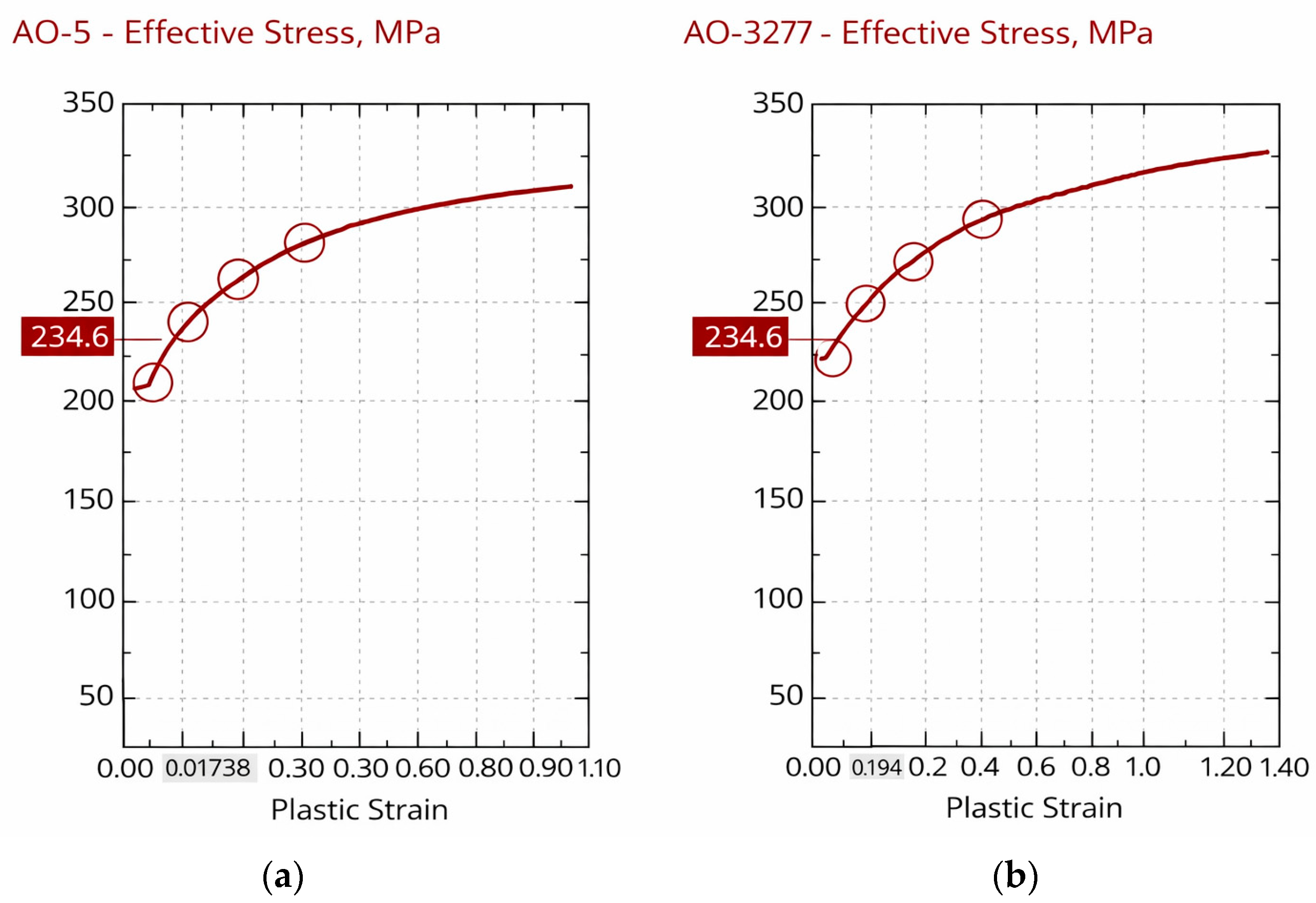
The graphical representation of the true diagrams (effective stress σ e q —plastic strain ϵ e q ) generated by the software during simulation modeling of the uniaxial tension test and pure twisting test for alloy AA7075 are shown in Figure 1.
A complete characterization of the process is performed by analyzing several moments from the indicator diagram and the true stress–strain diagram generated by the software, i.e., at different stages of deformation, namely, at the end of the yield stage; in the middle of the work hardening stage; at the beginning of the stage of localized deformation and/or when the plasticity limit is reached. In the true diagrams shown in Figure 1, the moments/stages at which the characteristics of the stress–strain state were analyzed are marked.
The specified mechanical deformation mode applies only to the stages of plastic deformation prior to the occurrence of stress concentration or loss of stability, since at these moments, the stress–strain state may undergo significant changes [6]. An exception is represented by impact toughness tests, as these evaluate the stress–strain state at the notch of the specimen. Although the determination of the strain rigidity also determines the type of fracture, it is generally accepted that its determination is not related to the process of crack initiation and propagation. Therefore, the application of the proposed classification is primarily related to interpreting and predicting the behavior of the material and the failure types based on simulation modeling.

3. Results and Discussion

3.1. Classification of Processes According to the Plastic Strain

All of the approaches described can be used to organize the processes, as they will be distinguished from one another; however, it is more important that they are grouped in such a way as to preserve the physical meaning of the stress–strain state. The classical approach to determining the efficiency of plastic deformation processes involves the use of the stress triaxiality parameter η σ , assessing the ratio of the hydrostatic stress σ m to the equivalent stress σ e q (7). In simulation modeling software, the values of these two scalar quantities are presented as the primary parameters for characterizing the stress state, while the other components of the stress tensor (such as the principal stresses) are obtained after the additional introduction of a material point into the deformed body.
The results of the simulation modeling were plotted in the presented diagrams using Graphing Calculator 3D v10.6 (Runiter Company, Cambridge, MA, USA).
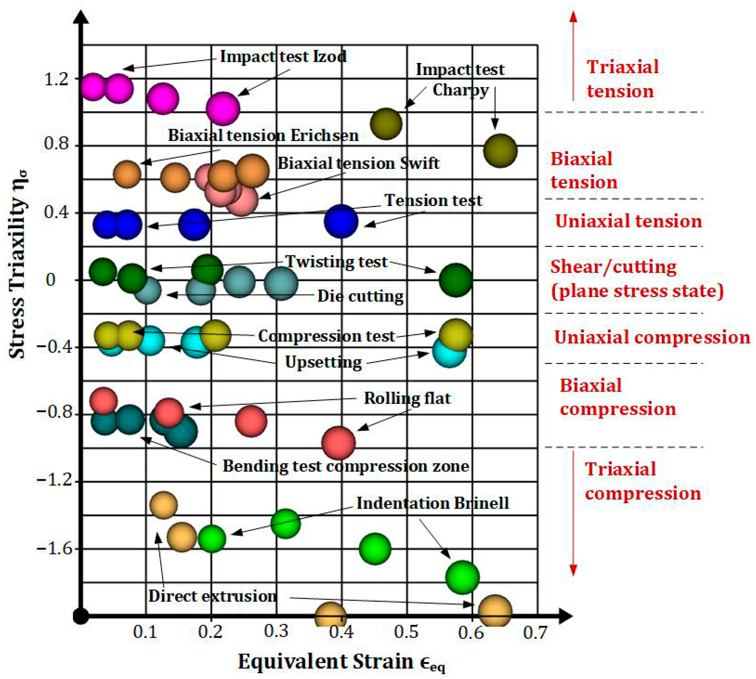
In plastic deformation processes, the stress–strain state is also influenced by the degree of deformation, as measured by the equivalent strain ϵ e q , which is a key parameter for describing the strain state in simulation modeling. In addition to the process’s ability to achieve certain degrees of strain without fracture, adding an abscissa axis with the values of ϵ e q to a plot with the ordinate of η σ (Figure 2) shows whether the deformation process is stationary or whether the stress state changes during plastic deformation.
The typical values of the stress triaxiality parameter, which distinguish the type of deformation processes based on the stress state, are as follows (Figure 2):   η σ 0 for the heterogeneous plane stress state of shear/cutting and for the twisting test, except when die-cutting values of −0.24 are reached;   η σ + 0.35 for uniaxial tension; and   η σ 0.33 for uniaxial compression, but reached at −0.38 during upsetting.
The plane stress states are located immediately above/below the uniaxial ones (Figure 2), namely, η σ 0.65 for biaxial tension; η σ 0.65 for biaxial compression.
The triaxial stress states originate from the plane stress state region and are not limited by the top or bottom of the graph (Figure 2), as follows: η σ 1.00 for triaxial tension (for example, in an impact test, it has a value of 1.15); η σ 1.00 for triaxial compression (for example, in direct extrusion, it reaches up to −2.00).
For the application of stress triaxiality η σ , the equivalent plastic strain ϵ e q groups deformation processes along lines of dots (Figure 2), which depend on the increasing degree of actual strain and are arranged one above the other depending on the type of stress state η σ . The lines characterizing the deformation processes are parallel or inclined lines, depending on the change in the stress state at different equivalent strain ϵ e q .

3.2. Classification of Processes Based on Stress–Strain State

Using the equivalent strain ϵ e q as the axis in the η σ ϵ e q diagram does not clearly distinguish the deformation processes, which are represented as overlapping lines (Figure 2). The classification of processes based on the stress–strain state must include a parameter that determines not only the type of stresses but also the type of strain state.
The inclusion of the strain rigidity coefficient α r i g (14) of the mode finalizes the classification of deformation processes for testing and pressure processing, allowing individual processes to be classified not only by the type of stress state but also by the type of strain state. An example of a classification of typical deformation processes in material testing and metal forming under pressure is presented in Table 1.
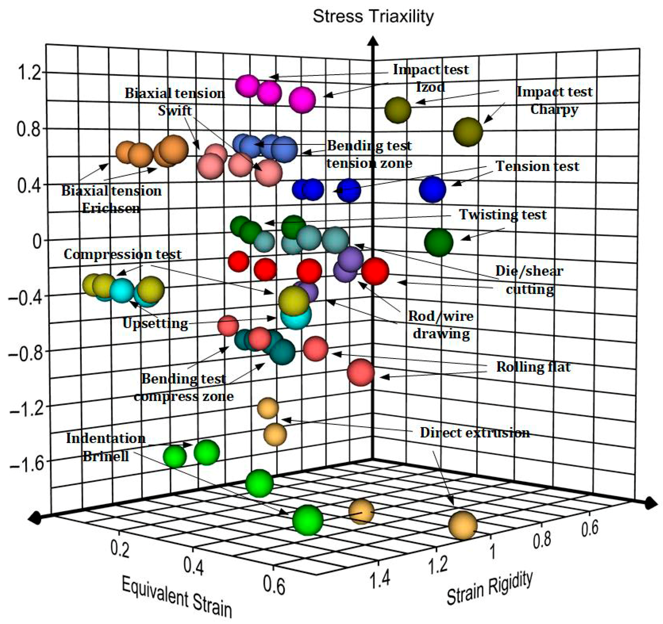
In addition to the graphical determination using the stress triaxiality parameter η σ and the equivalent strain ϵ e q , the ratio between the maximum shear and linear strains, which represents the strain rigidity coefficient α r i g of the mode, can also be included. The equivalent strain ϵ e q can be represented as a third axis in a 3D representation of the stress–strain state (Figure 3) or as depth in a 2D representation of the diagram η σ α r i g (Figure 4). The addition of a third axis adds depth to the 2D image but does not allow for clear differentiation and grouping of the individual deformation processes in the 3D diagram (Figure 3).
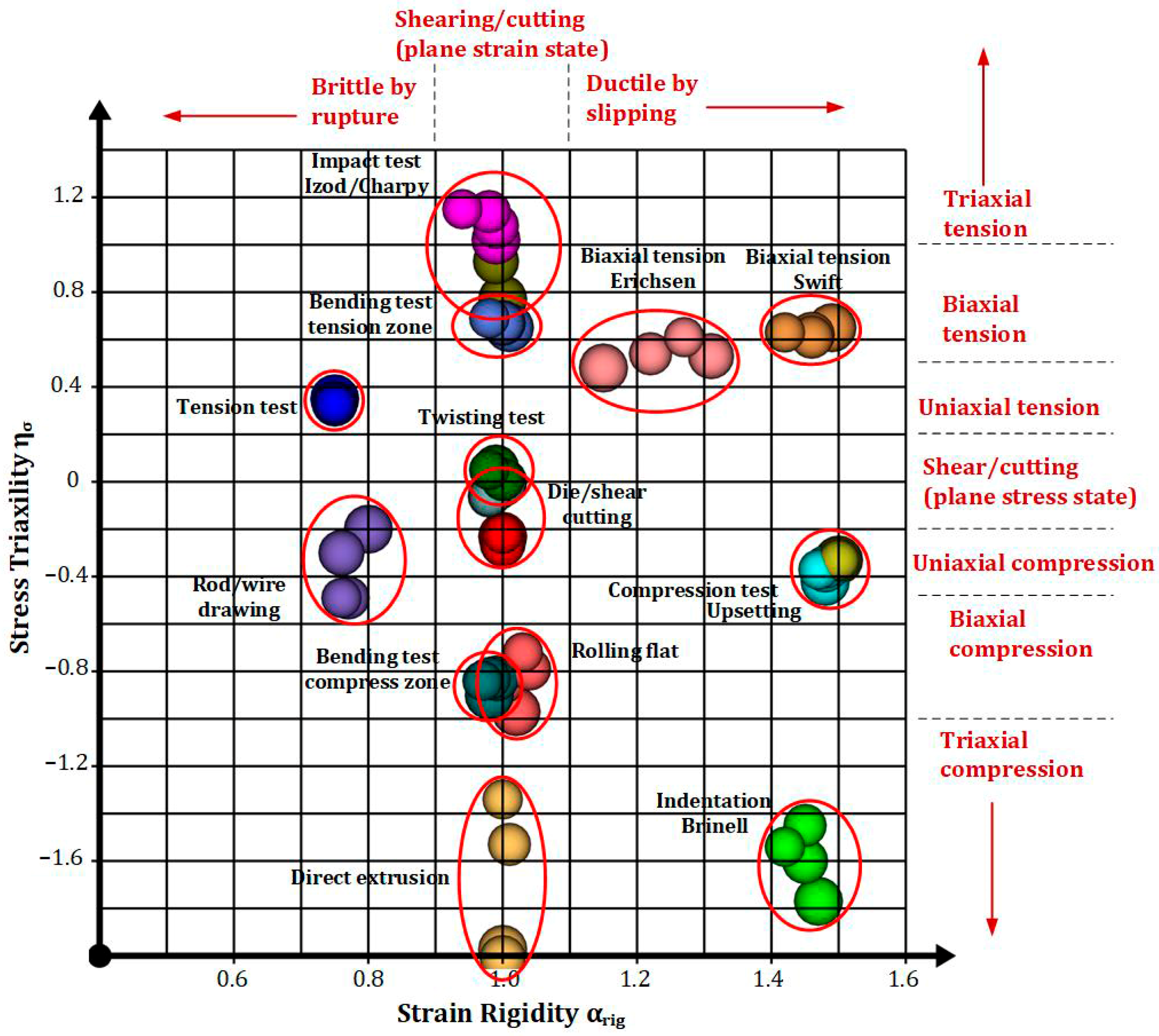
Creating a 2D diagram with the ordinate axis representing the stress triaxiality parameter η σ and the abscissa axis representing the strain rigidity coefficient α r i g allows for the visual differentiation of distinct zones that group various testing and pressure processing processes (Figure 4). The graphical 2D representation of the values in Table 1 allows for the identification of individual deformation processes in terms of their stress–strain state.
The ratio of maximum shear to maximum linear strains, defined by α r i g , also groups deformation processes according to the type of strain state, i.e., according to the type of fracture (Table 1), as follows: α r i g 0.75 —stretching, causing brittle fracture by rupture; α r i g 1.00 —deformation by shearing/cutting; and α r i g 1.50 —contraction, causing plastic fracture by slipping. While ζ ϵ varies between −1 (elongation) and +1 (contraction), and takes on values ζ ϵ 0 during shear (twisting), then α r i g ranges between 0.75 (stretching) and 1.5 (contraction), taking on values close to one during deformation shearing. However, the use of the strain rigidity α r i g to determine the strain state makes clear physical sense when determining strain shearing, since the maximum shear strain γ m a x is equal to the maximum linear strain ϵ m a x .
The third axis or the magnitude of the equivalent strain ϵ e q can be represented implicitly as an increasing size of the spheres/balls. Adding new spheres that represent the degree of strain as quasi-depth in the 2D plot indicates whether the deformation process is stationary (i.e., whether the circles overlap) or whether the stress state changes during the deformation process (i.e., whether the circles are separated from each other) (Figure 4).
When the degree of strain is implicitly accounted for, the static grouping of strain processes in the 2D plot of circles transforms into ellipsoidal zones with varying lengths and inclinations of the major axes (Figure 4). Potential applications of this classification include selecting an appropriate plastic deformation mode to achieve certain deformations, similar to the procedure for material selection in mechanical design.
It is clear that stationary processes form circles with a relatively small radius, whereas processes with a varying stress–strain state form ellipses as the degree of plastic strain increases (Figure 4).

3.3. Separation of Testing and Processing by Plastic Deformation Processes

The distinction between mechanical modes of deformation processes—such as those used for materials testing and those used for processing by plastic deformation—is purely arbitrary; however, the chosen classification method allows their specific characteristics to be highlighted.
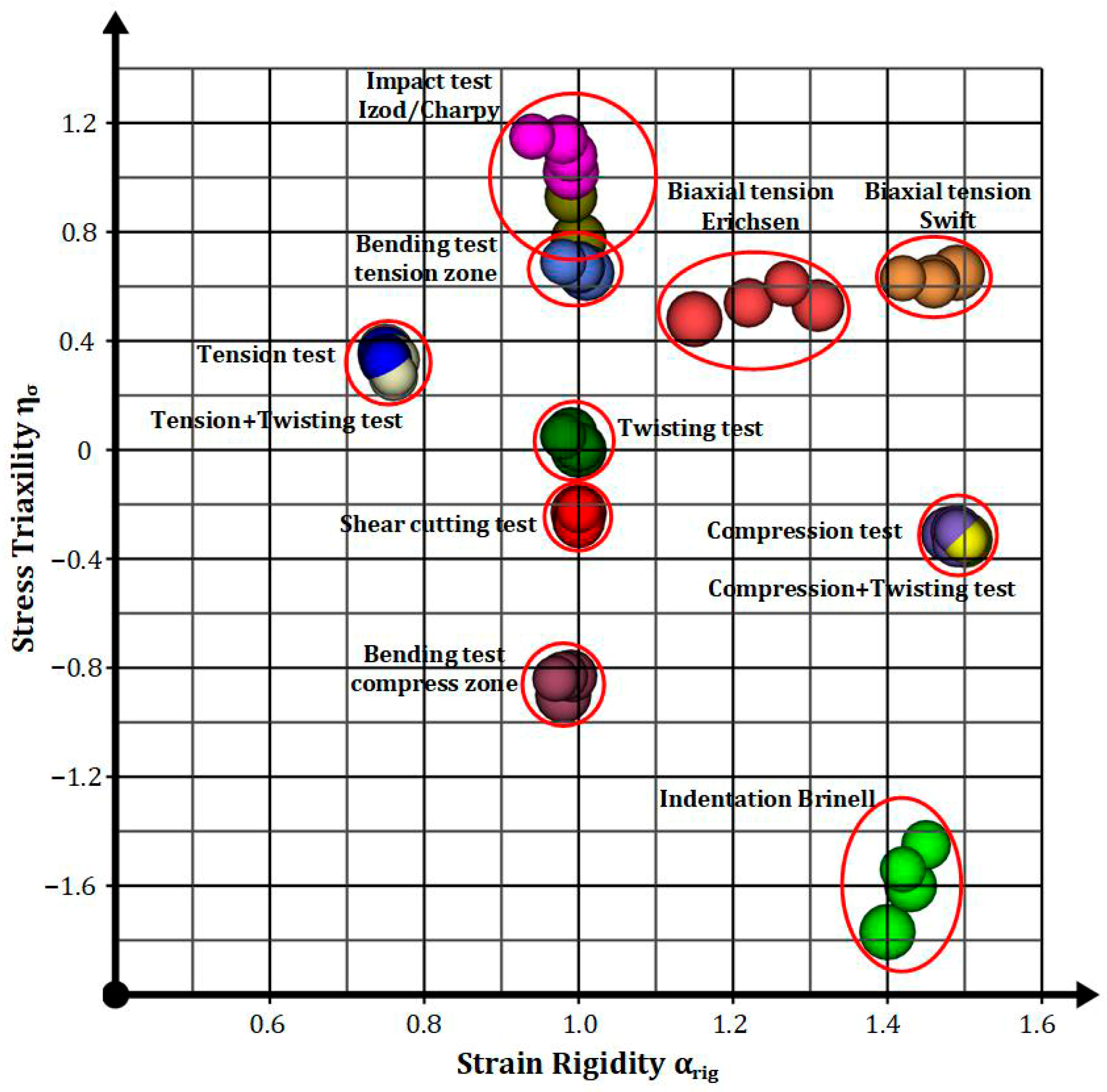
Deformation processes in material testing involving uniaxial or plane deformation modes are located in the middle and upper parts of the diagram (with the exception of indentation testing) (Figure 5). The static test modes for uniaxial tension and compression, as well as the biaxial mode for pure torsion and shear, are arranged such that their stress–strain state does not depend on the degree of strain; that is, they form circles with a small radius. This static behavior persists even under a combined deformation mode (tension + torsion and compression + torsion).
The static biaxial tension tests (Erichsen and Swift) are performed with a gradual change in the strain rigidity, and the triaxial tension in impact test (Charpy and Izod impact bending) is performed by changing the stress triaxiality in the notch (Figure 5).
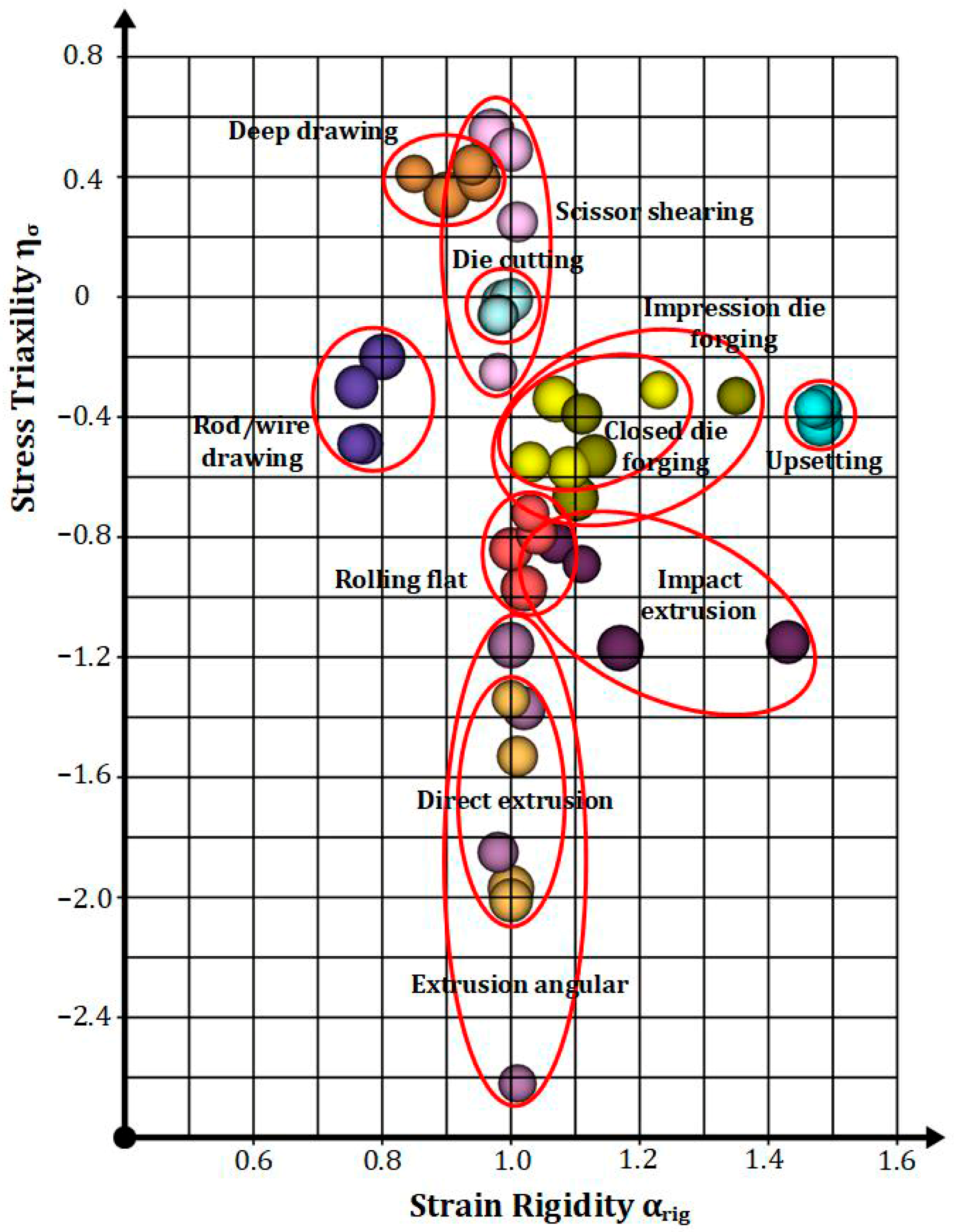
Processes for processing metals/alloys through plastic deformation are characterized by a variable stress–strain state that depends on the stage of deformation, i.e., on the degree of strain realized. With the exception of sheet metal shearing operations and deep drawing, they are concentrated mainly in the lower and middle parts of the diagram at negative values of the stress triaxiality parameter (Figure 6).
Figure 6 illustrates just one of the many processes involving severe plastic deformation (equal channel angular extrusion) to indicate the location of the mechanical mode with a distinctly negative spherical stress tensor. The classification of the remaining SPD processes would occupy the lower part of the graph, but their arrangement has been omitted in order to focus solely on classical processing by plastic deformation processes and to preserve the concept of verifying the graph itself.
All metalworking processes involving plastic deformation exhibit a progression through the various stages of deformation, as evidenced by the elongation of their elliptical zones. Unlike the testing, some of these processes inherently include and/or fully encompass other processes; that is, at a certain stage, they represent a variation in those processes in terms of their stress–strain state. These include processes for bulk deformation, such as direct and equal-channel angular extrusion, as well as various types of die forging (Figure 6). Similar grouping also includes cutting operations in sheet metal forming processes, such as shearing and die cutting, and for higher degrees of strain, the deep drawing process partially overlaps with this group (Figure 6).
As shown in the graphical representation using a plot with the ordinate axis representing the stress triaxiality parameter η σ and the abscissa axis representing the strain rigidity coefficient α r i g , supplemented (in depth) by accounting for the degree of strain ϵ e q , there is a distinct difference between the types of zones of the material testing processes groups (Figure 5) and those for processing by plastic deformation (Figure 6). These differences only emphasize the characteristic features of the structure and purpose of the two types of deformation processes, which at first glance appear to be identical.

4. Conclusions

  • A relationship has been identified that determines the value of the strain rigidity coefficient α r i g , which represents a further development of the idea of classifying strain state by supplementing the strength theory, of the following form:
    γ m a x ϵ m a x = 3 4 σ 1 σ 3 σ 1 ½ σ 2 + σ 3 ,
    providing a more direct relationship between the maximum shear strain γ m a x and the maximum linear strain ϵ m a x , grouping the deformation processes according to the type of fracture caused.
  • Virtual solutions have been developed for the main deformation processes involved in processes for testing and processing by plastic deformation of metals and alloys, which have been implemented through simulation modeling within the software platform Quantor Form 8.2.4.
  • A classification of typical deformation processes is proposed through the quantitative determination of the stress triaxiality parameter η σ and the strain rigidity coefficient α r i g , taking into account the degree of equivalent strain ϵ e q achieved.
  • It has been established that the graphical representation of diagrams η σ α r i g allows for the classification of deformation processes by determining the type of stress–strain state of the corresponding mechanical mode using simulation modeling.
  • Through simulation modeling using the appropriate virtual tools, it has been confirmed that the deformation processes during the testing of metals and alloys (using uniaxial or plane strain mode) are located in the middle and upper regions of the η σ α r i g diagrams and are organized in such a way that their stress–strain state remains unchanged under various degrees of equivalent strain ϵ e q before they lose stability.
  • Through simulation modeling using the appropriate virtual tools, it has been confirmed that the fundamental processes of processing by plastic deformation of metals and alloys are characterized by a variable stress–strain state, which depends on the degree of strain, as they encompass and/or fully cover other processes; i.e., at a certain stage, they represent a variant of those processes.

Author Contributions

Conceptualization, V.K. and R.D.; methodology, V.K.; software, V.K.; validation, R.D. and V.K.; formal analysis, V.K.; investigation, V.K.; resources, R.D.; data curation, R.D.; writing—original draft preparation, V.K.; writing—review and editing, V.K. and R.D.; visualization, R.D.; supervision, V.K.; project administration, V.K.; funding acquisition, R.D. All authors have read and agreed to the published version of the manuscript.

Funding

This work has been accomplished with financial support by the European Regional Development Fund within the Operational Programme “Bulgarian national recovery and resilience plan”, procedure for direct provision of grants “Establish of a network of research higher education institutions in Bulgaria”, and under Project BG-RRP-2.004-0005 “Improving the research capability anD quality to achieve intErnAtional recognition and reSilience of TU-Sofia (IDEAS)”.

Data Availability Statement

The original contributions presented in this study are included in the article. Further inquiries can be directed to the corresponding author.

Acknowledgments

The research and preparation of this article were funded by Project BG-RRP2.004 0005 “Improving the research capacity and quality to achieve intErnAtional recognition and reSilience of TU-Sofia (IDEAS)”. The software used for this study is the computer-aided engineering product Quantor Form 8.2.4, designed for the simulation modeling of plastic deformation processes in metals and their alloys.

Conflicts of Interest

The authors declare no conflicts of interest.

Abbreviations

The following abbreviations are used in this manuscript:
σ 1 ,   σ 2 ,   σ 3 principal normal stresses
τ 12 ,   τ 23 ,   τ 13 principal shear stresses
σ e q von Mises equivalent stress
σ m mean (hydrostatic) stress
ζ σ stress Lode–Nadai parameter
J 1 ,   J 2 ,   J 3 deviatoric stress tensor invariants
ϵ 1 ,   ϵ 2 ,   ϵ 3 principal true strains
γ 12 ,   γ 23 ,   γ 13 principal shear strains
ζ ϵ strain Lode–Nadai parameter
ν Poisson’s ratio
G second-order modulus of plasticity
η σ stress triaxiality
α r i g strain rigidity coefficient

References

  1. Hill, R. The Mathematical Theory of Plasticity; Oxford University Press: Oxford, UK, 1998. [Google Scholar] [CrossRef]
  2. Storozhev, M.; Popov, E. Teopия oбpaбoтки мeтaллoв дaвлeниeм [Theory of Metal Pressure Processing], 4th ed.; Meshterin, V., Ed.; Mashinostroenie Press: Moscow, Russia, 1977. (In Russian) [Google Scholar]
  3. Chakrabarty, J. Theory of Plasticity, 3rd ed.; Elsevier Butterworth-Heinemann: Oxford, UK, 2006. [Google Scholar]
  4. Kalpachjian, S.; Schmid, S. Manufacturing Processes for Engineering Materials, 5th ed.; Pearson Education Inc.: London, UK; Prentice Hall: Hoboken, NJ, USA, 2008. [Google Scholar]
  5. Genov, J.; Kamburov, V. Oбpaбoтвaнe нa мeтaлитe чpeз плacтичнa дeφopмaция [Processing of Metals by Plastic Deformation]; Tontchev, N., Ed.; Technical University of Sofia Press: Sofia, Bulgaria, 2019. (In Bulgarian) [Google Scholar]
  6. Hristov, S. Изпитвaнe и дeφeктocкoпия нa мeтaлитe [Testing and Non-Destructive Testing of Metals]; Higher Institute of Mechanical and Electrical Engineering Press: Sofia, Bulgaria, 1988. (In Bulgarian) [Google Scholar]
  7. Kisyov, I. Cъпpoтивлeниe нa мaтepиaлитe [Strength of Materials]; Popov, B., Ed.; State Publishing House Technika: Sofia, Bulgaria, 1970. (In Bulgarian) [Google Scholar]
  8. Friedman, Y.B. Mexaничecкиe cвoйcтвa мeтaллoв [Mechanical Properties of Metals]; Mashinostroenie Press: Moscow, Russia, 1974. (In Russian) [Google Scholar]
  9. Dowling, N. Mechanical Behavior of Materials: Engineering Methods for Deformation, Fracture and Fatique, 4th ed.; Pearson Educational Ltd.: London, UK, 2013. [Google Scholar]
  10. Gere, J.M.; Goodno, B.J. Mechanics of Materials, 8th ed.; Global Engineering: Shelby Township, MI, USA, 2013. [Google Scholar]
  11. White, G.N.; Drucker, D.C. Effective stress and effective strain in relation to stress theories of plasticity. J. Appl. Phys. 1950, 21, 1013–1021. [Google Scholar] [CrossRef]
  12. Hill, R. A remark on diagonal streaming in plane plastic strain. J. Mech. Phys. Solids 1966, 14, 245–248. [Google Scholar] [CrossRef]
  13. Alexandrov, S.; Rynkovskaya, M.; Li, Y. Principal Stress Trajectories in Plasticity under Plane Strain and Axial Symmetry. Symmetry 2023, 15, 981. [Google Scholar] [CrossRef]
  14. Mises, R. Mechanik der festen Körper im plastisch-deformablen Zustand. Nachrichten Ges. Wiss. Gött. Math.-Phys. Kl. 1913, 1, 582–592. [Google Scholar]
  15. Ford, H. Advanced Mechanics of Materials; Longmans: London, UK, 1963. [Google Scholar]
  16. Lode, W. Versuche über den Einfluß dermittleren Hauptspannung auf das Fließen der Metalle Eisen, Kupfer und Nickel. Z. Phys. 1926, 36, 913–939. [Google Scholar] [CrossRef]
  17. Kim, J.; Nguyen, P.V.; Hong, J.G.; Kim, Y.S. Stress-Invariants-Based Anisotropic Yield Functions and Its Application to Sheet Metal Plasticity. Metals 2023, 13, 142. [Google Scholar] [CrossRef]
  18. Bao, Y.B.; Wierzbicki, T. On fracture locus in the equivalent strain and stress triaxiality space. Int. J. Mech. Sci. 2004, 46, 81–98. [Google Scholar] [CrossRef]
  19. Bruhns, O.T. Some remarks on Lode angle and Lode parameter. Proc. Appl. Math. Mech. 2024, 2, e202400004. [Google Scholar] [CrossRef]
  20. Peng, J.; Zhou, P.; Wang, Y.; Dai, Q.; Knowles, D.; Mostafavi, M. Stress Triaxiality and Lode Angle Parameter Characterization of Flat Metal Specimen with Inclined Notch. Metals 2021, 11, 1627. [Google Scholar] [CrossRef]
  21. Xing, M.; Liu, Y.; Lu, J.; Huang, X.; Wang, X.; Xue, J.; Zhang, F.; Du, F. Fracture Criterion Calibration and Finite Element Simulation in SUS304 Stainless Steel. Materials 2024, 17, 5711. [Google Scholar] [CrossRef] [PubMed]
  22. Peng, J.; Wang, Y.; Dai, Q.; Liu, X.; Liu, L.; Zhang, Z. Effect of Stress Triaxiality on Plastic Damage Evolution and Failure Mode for 316L Notched Specimen. Metals 2019, 9, 1067. [Google Scholar] [CrossRef]
  23. Huang, J.; Guo, Y.; Qin, D.; Zhou, Z.; Li, D.; Li, Y. Influence of stress triaxiality on the failure behavior of Ti-6Al-4V alloy under a broad range of strain rates. Theor. Appl. Fract. Mech. 2018, 97, 48–67. [Google Scholar] [CrossRef]
  24. González, Á.; Celentano, D.; Cruchaga, M.; Ponthot, J.-P. The Triaxiality Effect on Damage Evolution in Al-2024 Tensile Samples. Metals 2024, 14, 1103. [Google Scholar] [CrossRef]
  25. Zhang, H.; Zhang, H.; Li, F.; Cao, J. A Novel Damage Model to Predict Ductile Fracture Behavior for Anisotropic Sheet Metal. Metals 2019, 9, 595. [Google Scholar] [CrossRef]
  26. Baruscotti, A.; Miori, N.; Concli, F. Determination of the Fracture Locus of a Cor-Ten Steel at Low and High Triaxiality Ranges. Appl. Sci. 2025, 15, 3569. [Google Scholar] [CrossRef]
  27. Rickhey, F.; Hong, S. Stress Triaxiality in Anisotropic Metal Sheets—Definition and Experimental Acquisition for Numerical Damage Prediction. Materials 2022, 15, 3738. [Google Scholar] [CrossRef] [PubMed]
  28. Segal, V. Review: Modes and Processes of Severe Plastic Deformation (SPD). Materials 2018, 11, 1175. [Google Scholar] [CrossRef] [PubMed]
  29. Kamburov, V. Teopeтични acпeкти и виpтyaлни peшeния зa интeнзивнa плacтичнa дeφopмaция c peдyциpaни и aктивни cили нa тpиeнe [Theoretical Aspects and Virtual Solutions for Severe Plastic Deformation with Reduced and Active Friction Forces]; Genov, J., Ed.; Copy Print Studio: Sofia, Bulgaria, 2021. (In Bulgarian) [Google Scholar]
  30. Alomari, Q.A.; Yosef, T.Y.; Bielenberg, R.W.; Faller, R.K.; Negahban, M.; Zhang, Z.; Li, W.; Humphrey, B.M. Material Characterization and Stress-State-Dependent Failure Criteria of AASHTO M180 Guardrail Steel: Experimental and Numerical Investigation. Materials 2025, 18, 2523. [Google Scholar] [CrossRef] [PubMed]
  31. Friedlein, J.; Böhnke, M.; Schlichter, M.; Bobbert, M.; Meschut, G.; Mergheim, J.; Steinmann, P. Material Parameter Identification for a Stress-State-Dependent Ductile Damage and Failure Model Applied to Clinch Joining. J. Manuf. Mater. Process. 2024, 8, 157. [Google Scholar] [CrossRef]
Figure 1. The true stress–strain curves during testing of deformable work-hardening AA7075 (a) in uniaxial tension tests; (b) in pure twisting test (QForm 8.2.4).
Metals 16 00445 g001
Figure 2. Graphical 2D representation of plastic deformation processes as a function of the stress triaxiality parameter η σ and the equivalent strain ϵ e q (QForm 8.2.4—alloy AA7075).
Metals 16 00445 g002
Figure 3. Graphical 3D representation of plastic deformation processes as a function of the stress triaxiality parameter η σ , the equivalent strain ϵ e q and the strain rigidity coefficient α r i g (QForm 8.2.4—alloy AA7075).
Metals 16 00445 g003
Figure 4. Graphical representation of the stress–strain state of deformation processes, defined by the stress triaxiality parameter η σ and the strain rigidity coefficient α r i g (QForm 8.2.4—alloy AA7075).
Metals 16 00445 g004
Figure 5. Graphical representation of the stress–strain state of material testing processes, determined by the stress triaxiality parameter η σ and the strain rigidity coefficient α r i g (QForm 8.2.4—alloy AA7075).
Metals 16 00445 g005
Figure 6. Graphical representation of the stress–strain state of processing operations by plastic deformation, determined the stress triaxiality parameter η σ and the strain rigidity coefficient α r i g (QForm 8.2.4—alloy AA7075).
Metals 16 00445 g006
Table 1. Classification of plastic deformation processes based on the stress triaxiality parameter η σ and the strain rigidity coefficient α r i g (QForm 8.2.4—alloy AA7075).
The Stress State ModeExample of a Deformation ProcessStress Triaxiality
Parameter η σ
Strain Rigidity
Coefficient α r i g
triaxial tensionimpact test (Izod)1.00 ÷ 1.150.97
impact test (Charpy)0.70 ÷ 0.931.00
biaxial tensiontension zone in bending0.65 ÷ 0.691.00
biaxial tension test (Erichsen)0.63 ÷ 0.651.24
biaxial tension test (Swift)0.48 ÷ 0.611.46
uniaxial tensiontension test0.330.75
heterogeneous plane statepure twisting test0.01 ÷ 0.050.99
shear/cutting test−0.22 ÷ −0.271.00
die-cutting−0.11 ÷ −0.330.99
uniaxial compressioncompression test−0.331.50
upsetting−0.36 ÷ −0.421.48
biaxial compressioncompression zone in bending−0.83 ÷ −0.900.98
flat rolling−0.72 ÷ −0.971.02
triaxial compressiondirect extrusion−1.34 ÷ −2.011.00
equal-channel angular extrusion−1.37÷ −2.621.00
Disclaimer/Publisher’s Note: The statements, opinions and data contained in all publications are solely those of the individual author(s) and contributor(s) and not of MDPI and/or the editor(s). MDPI and/or the editor(s) disclaim responsibility for any injury to people or property resulting from any ideas, methods, instructions or products referred to in the content.