Ductile Fracture Prediction for Ti6Al4V Alloy Based on the Shear-Modified GTN Model and Machine Learning

Abstract

To investigate the failure behavior of Ti6Al4V alloy under complex stress states, this study designed tensile specimens with different notches to achieve high, medium, and low stress triaxiality conditions. By adjusting the width of the notch spacing of the specimens, the failure mode can be transformed from tension-dominated fracture to shear stress-dominated fracture, which enables further examination of the damage model’s effectiveness. A shear-modified Gurson–Tvergaard–Needleman (GTN) model was employed to predict the failure behavior under various stress states. For calibrating the GTN parameters, a machine learning approach was adopted. Back propagation (BP) neural networks were used to construct surrogate models for predicting the fracture strains of three typical specimens, and genetic algorithms (GAs) were integrated for optimization, to minimize the discrepancy in fracture strains between experimental results and finite element analysis (FEA). Finally, an optimal set of parameters was determined. This set of parameters can effectively predict the failure behavior of all specimens, including not only the stress–strain curves, but also the failure modes (fracture locations).

1. Introduction

Titanium alloys are vital structural materials widely used in aerospace, mechanical engineering, marine, and biomedical sectors due to their high strength-to-density ratios, excellent corrosion resistance, and superior mechanical properties [1,2,3]. However, during service, components experience complex loading, leading to the initiation and accumulation of localized micro-damage. This damage accumulation acts as a precursor to crack nucleation and propagation, ultimately becoming the dominant failure mechanism and potentially causing catastrophic in-service failures [4,5,6]. Thus, a thorough understanding of titanium alloy deformation and damage accumulation under various stress states is crucial. Furthermore, establishing an effective damage constitutive model to predict the failure behavior of titanium alloy structures under complex loading conditions is of significant engineering importance for ensuring their safety and reliability [5,7].

Current models for ductile fracture fall into two primary categories, based on their construction approach: continuous damage mechanics (CDM) [8,9,10,11] models and phenomenological mesoscopic damage models [12,13,14,15]. CDM, also termed macroscopic damage mechanics, is grounded in continuum mechanics and thermodynamics [16,17]. It conceptualizes microstructural changes during plastic deformation as an irreversible dissipative process. These models primarily focus on damage’s impact on macroscopic mechanical properties and its evolution, employing internal variables to bridge micro/mesoscopic damage processes with macroscopic analysis [18,19,20]. Kachanov et al. [21] introduced a damage quantification method comparing effective load-bearing area to original surface area to determine fracture onset. A key limitation, however, is the model’s inability to geometrically characterize internal damage evolution.

Mesoscopic damage models can be further divided into uncoupled and coupled types, based on the relationship between mesoscopic void evolution and macroscopic material degradation [22,23,24]. The void growth model (VGM) is a widely used uncoupled mesoscopic damage model [14]. It neglects the degradation of material mechanical properties during void evolution and calculates the fracture index (void volume fraction, VVF) based on the mechanical properties of undamaged materials. While uncoupled mesoscopic damage models feature simple parameters that are easy to calibrate, their accuracy is often limited [24]. In contrast, the Gurson–Tvergaard–Needleman (GTN) model stands as a classic coupled damage model, initially proposed by A. L. Gurson and later refined by V. Tvergaard and A. Needleman [12,13]. It fully accounts for the complete evolution process of microvoids, including nucleation, growth, and coalescence, and has been widely applied in the simulation of ductile fracture.

However, although the GTN model exhibits high accuracy in simulating fracture behavior under medium and high stress triaxiality conditions, it fails to effectively predict fracture behavior under low stress states, due to its inability to describe void evolution processes under shear stress [25,26,27,28], as shown in Figure 1. In CDM, the Lode angle (i.e., the third invariant of the deviatoric stress tensor) is often introduced to modify the damage evolution equation, thereby improving its accuracy under low stress triaxiality conditions [23,29,30]. Similarly, Nahshon and Hutchinson [31] extended the GTN model by utilizing the third invariant of stress to distinguish shear-dominated states, incorporating the effective damage accumulation induced by the void shear mechanism. Xue [32] defined a new shear damage variable based on a unity cell analysis and combined it with the VVF to construct a total damage variable in the modified GTN model. These optimizations have effectively enhanced the applicability of the GTN model under low stress triaxiality conditions [25,26,27,33,34,35].

The calibration of parameters in the GTN model is always a challenging task, and the introduction of shear correction terms has further increased the number of parameters. Researchers have employed various mesoscopic analysis methods, such as X-ray tomography and scanning electron microscopy (SEM), to directly determine the parameters in the GTN model [5,36,37], as shown in Figure 2. For instance, Cao et al. [38] quantified the initial, critical, and final void volume fractions of 6061 aluminum alloy during tensile processes through in situ X-ray micro-tomography and SEM tests. However, the entire testing process is extremely costly and time-consuming. The inverse analysis method, which calibrates model parameters by matching FEA results with experimental results from typical tests under simple stress states (such as uniaxial tension), is also a widely accepted approach for identifying GTN model parameters [7,25,34]. For example, Ding et al. [34] used a FEA inversion method to determine parameters related to the hardening law, tensile damage, and shear damage in the shear-modified GTN model. Nevertheless, traditional inverse analysis requires multiple iterations of FEA calculations, with parameter adjustments in each iteration, making it quite time-consuming. Additionally, parameter adjustment is prone to falling into local optimal solutions. Machine learning methods, such as neural networks and genetic algorithms (GA), as novel approaches, are being increasingly widely applied in the calibration of damage models with multiple parameters [23,33,39,40,41,42].

In this study, tensile specimens with different notch configurations were designed to achieve high, medium, and low stress triaxiality states. The shear-modified GTN model was adopted to simulate the failure behavior of these notched specimens. A parameter calibration framework integrating back propagation (BP) neural networks and GAs was proposed: surrogate models for calculating the fracture strains of three typical specimens were constructed using BP neural networks, and GAs were employed to minimize the discrepancy in fracture strains between experimental results and FEA. An optimal set of parameters was determined, and the validity of these parameters was verified using the remaining specimens.

2. Materials and Methods

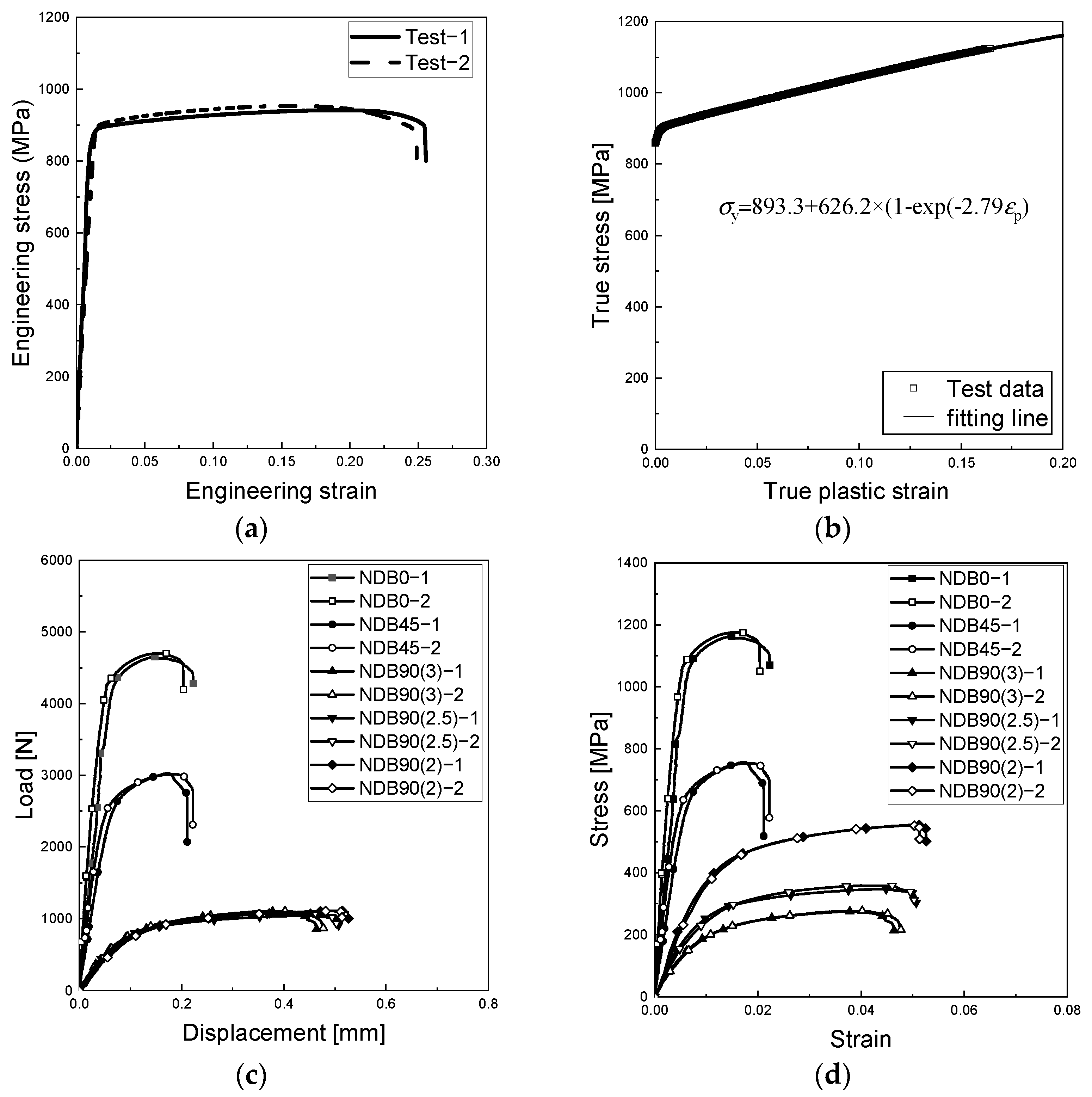
Titanium alloys are widely used structural materials due to their excellent mechanical properties. Among them, Ti-6Al-4V, as the most widely used and technologically mature titanium alloy, accounts for approximately 55% of the total application of structural materials [1]. In this study, all tensile specimens were obtained from 2 mm thick Ti6Al4V sheets. To simplify the model, anisotropic behavior, which Ti6Al4V may exhibit due to its microstructure, was not explicitly incorporated. However, to minimize the impact of anisotropy, all specimens were cut in the same orientation. The chemical composition of Ti6Al4V is listed in

Table 1. Chemical composition of Ti6Al4V sheet (weight %).

Element	Al	V	Fe	C	Sn	O	N	Ti
Wt (%)	5.8~6.5	3.8~4.5	≤0.30	≤0.08	≤0.07	0.10~0.15	≤0.05	rest

. Smooth dog bone (SDB) and notched dog bone (NDB) specimens with various notch geometries were used to investigate the mechanical and fracture properties, as shown in Figure 3. SDB specimens (Figure 3a) were tested to obtain the yielding and hardening properties, as shown in Figure 4a. The resulting Young’s modulus, yield strength, and tensile strength were determined to be 109.5 GPa, 893.3 MPa, and 953.2 MPa, respectively. The hardening model of Voce was applied to fit the stress–strain curve, as displayed in Figure 4b.

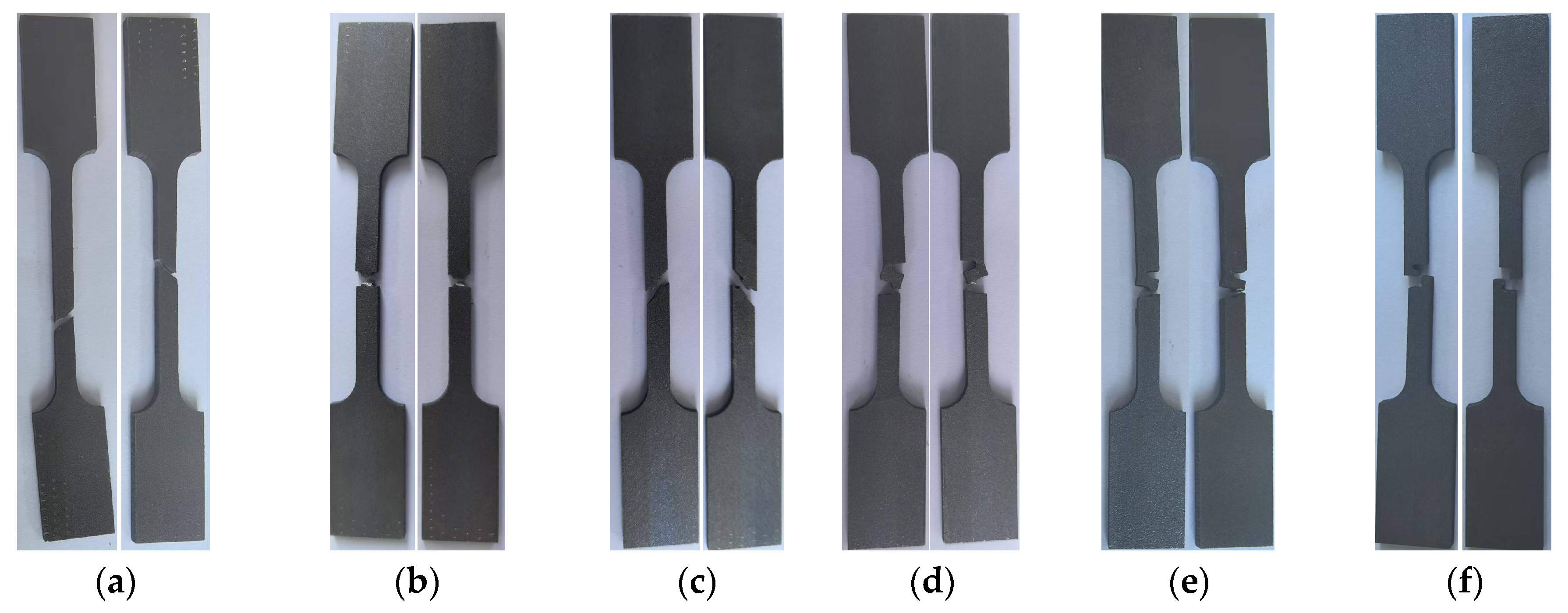
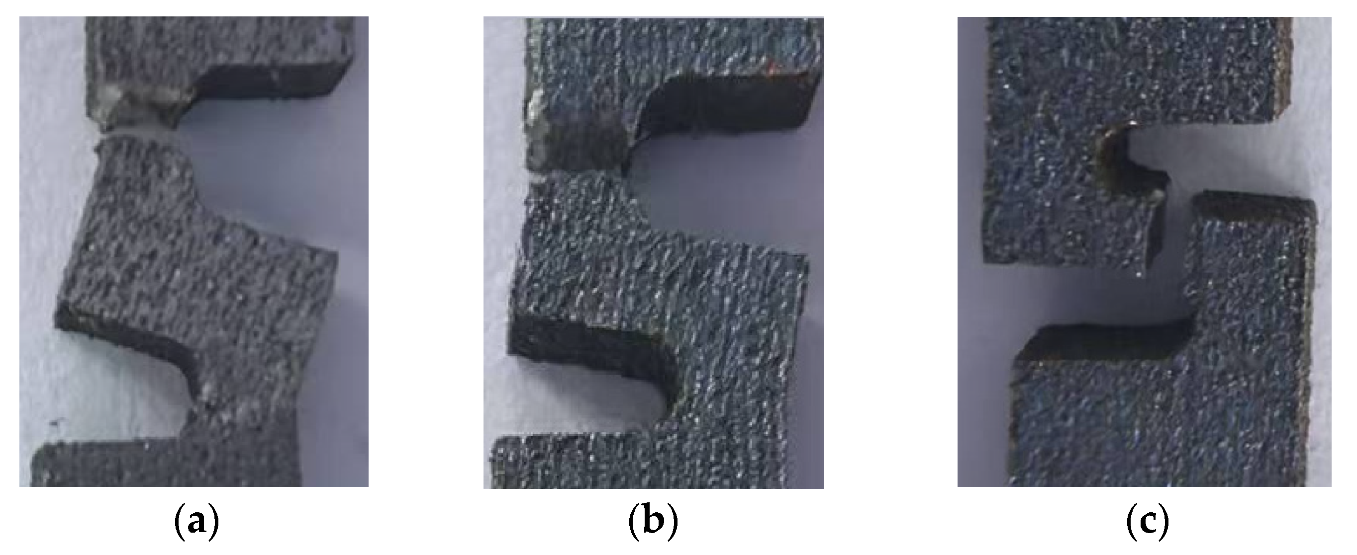
The notch geometries of NDB specimens were designed to cover various stress triaxiality conditions. In addition, the specimens of (d), (e), (f), with varying notch spacings, were used to distinguish whether shear stress dominated the void growth process. The loading rate was controlled by the crosshead at a velocity of 1 mm/min to maintain quasi-static conditions. Displacement was measured using a 10 mm gauge length extensometer with an accuracy of ±0.5 µm, while force was recorded via a 10 kN capacity load transducer accurate to ±0.1% of full scale. The resulting load–displacement curves are presented in Figure 4c. The stress–strain curves for all the notched specimens are displayed Figure 4d, where the strain represents the average value within the gauge section measured by the extensometer, and the stress is calculated as the load divided by the effective cross-sectional area at the notch. Although it is standard practice to conduct triplicate tests for mechanical characterization, two tests were performed for each of the six specimen geometries in this study, as both tests demonstrated good consistency and were deemed sufficient for comparative analysis. Figure 5 displays the fracture specimens. As observed, the specimens of NDB90(3), NDB90(2.5), and NDB90(2), with progressively decreasing notch spacing, exhibited a transition in failure location, shifting from tension-dominated fracture to shear-dominated fracture, as shown in Figure 6.

3. Shear-Modified GTN Model

A GTN model simulates ductile fracture by modeling the formation, growth, and coalescence of microvoids [13]. It integrates the void volume fraction (VVF) into the yield function, directly accounting for void evolution’s impact on plastic behavior.

$$\mathsf{\Phi }={({\displaystyle \frac{{\sigma }_{eq}}{{\sigma }_y}})}^2+2q_1{f}^{*}cosh({\displaystyle \frac{3q_2{\sigma }_m}{2{\sigma }_y}})-1-{(q}_1{f^{*})}^2$$

(1)

where $q_1$ and $q_2$ are parameters relating to the hardening of the material; ${\sigma }_{eq}$ and ${\sigma }_m$ are the Huber–von Mises stress and the hydrostatic stress; ${\sigma }_y$ is the yield stress of the material; and $f^{*}$ is a function of the VVF (f), as follows:

$$f^{*}=\left\{\begin{array}{c} f { f}_0\le f\le f_c\\ f_c+k(f-f_c) f_c<f \end{array}\right.$$

(2)

where $f_0$ is the initial VVF, and $f_c$ is the critical VVF for void coalescence. When the VVF reaches $f_c$, the interaction between microvoids occurs, and the void growth will be accelerated by a factor $k$, as follows:

$$k={\displaystyle \frac{f_u^{*}-f_c}{f_F-f_c}}$$

(3)

where $f_u^{*}$ = 1/$q_1$, and $f_F$ defines the VVF at final failure of the material. In the conventional GTN model, VVF of the material increases, due to either the nucleation of new voids at material defects,$d{f}_{nucl}$, or the growth of the voids pre-existing in the material, $d{f}_{gr}$, as follows:

$$d{f}_{nucl}={\displaystyle \frac{f_N}{s_N\sqrt{2\pi }}}exp[-{\displaystyle \frac{1}{2}}{({\displaystyle \frac{{\epsilon }_m^p-{\epsilon }_N}{s_N}})}^2]d{\epsilon }_m^p$$

(4)

$$d{f}_{gr}=(1-f)d{\mathsf{\epsilon }}^{\mathit{p}}:\mathbf{I}$$

(5)

where $f_N$ is the the possible nucleated VVF; ${\epsilon }_m^p$ is the equivalent plastic strain of the matrix; ${\epsilon }_N$ and $s_N$ are the average equivalent plastic strain and the standard deviation of the nucleation strain during nucleation; ${\mathsf{\epsilon }}^{\mathit{p}}$ is the plastic strain tensor; and I is the second-order unit vector.

In the conventional GTN model, the growth rate of VVF vanishes when the hydrostatic stress is zero. This indicates that no damage should develop under zero stress triaxiality, contradicting the observed phenomenon of shear fracture in materials [26,27]. To address this limitation, Nahshon and Hutchinson [31] developed the shear-modified GTN model. This model incorporates the influence of shear damage on void volume by introducing the driving effect of shear stress on void evolution, in addition to the original mechanisms of void nucleation and growth.

$$df=d{f}_{nucl}+d{f}_{gr}+d{f}_s$$

(6)

where $d{f}_s$ is the shear-induced increment of VVF. It can be calculated as follows:

$$d{f}_s=k_{w}fw(\sigma ){\displaystyle \frac{\mathit{s}:d{\mathsf{\epsilon }}^{\mathit{p}}}{{\sigma }_{eq}}}$$

(7)

where $k_w$ is the shear damage parameter, and s is the deviatoric stress tensor. $w\left(\sigma \right)$ represents a stress state weighting function, expressed as follows:

$$w(\sigma )=1-{({\displaystyle \frac{27J_3}{2{\sigma }_{eq}^3}})}^2$$

(8)

where $J_3$ is the third invariant of the deviatoric stress tensor, which governs the activation of shear damage. $w\left(\sigma \right)$ ranges continuously between 0 and 1, vanishing ($w\left(\sigma \right)$ = 0) during uniaxial tension, where $J_3=2{\sigma }_{eq}^3/27$, and reaching unity ($w\left(\sigma \right)$ = 1) under pure shear ($J_3$ = 0). Consequently, $f_s$ is suppressed in tensile states, but dominates in shear-driven failure. This extension resolves the conventional GTN model’s limitation in predicting ductile fracture under low stress triaxiality loading. This constitutive model was numerically implemented in Abaqus/Explicit via a user-defined VUMAT subroutine.

4. Finite Element Analysis

4.1. Finite Element Modeling

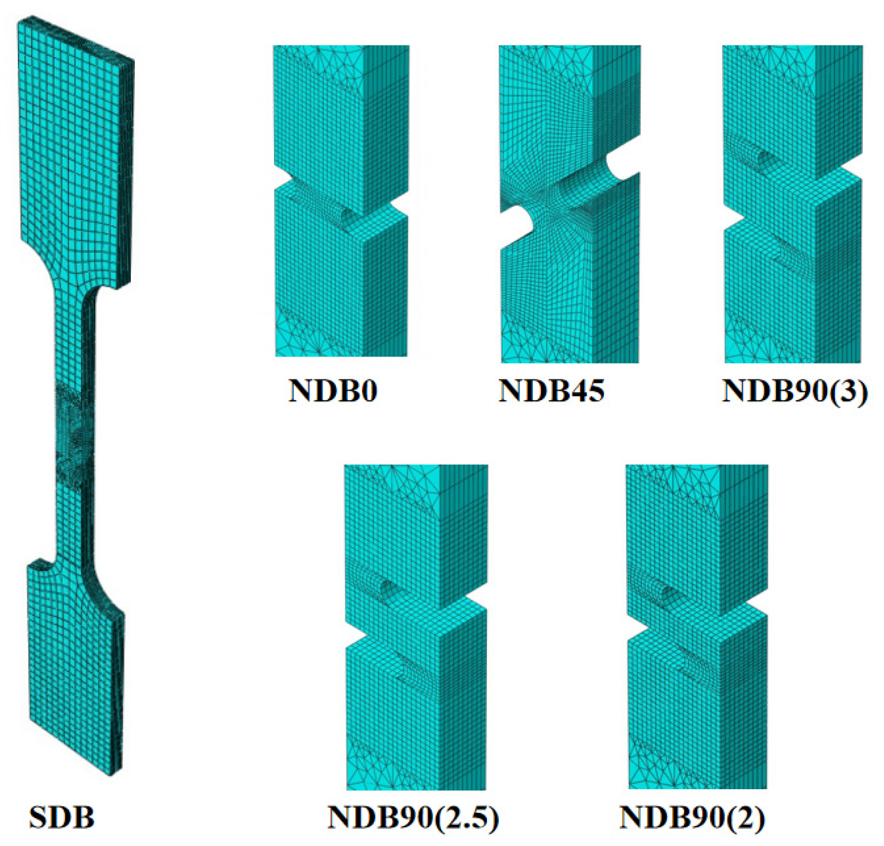
3D FEA models of SDB and NDB specimens were constructed in ABAQUS/CAE. The dimensions were the same as those given in Figure 1. As shown in Figure 7, the gauge section was discretized using C3D8R elements (8-node linear brick elements with reduced integration). The C3D8R element was chosen for its computational efficiency and ability to capture large plastic deformation without volumetric locking. A convergence study was carried out by progressively refining the mesh until the change in equivalent strain was negligible. A mesh size of 0.2 mm was ultimately selected. Boundary conditions followed those applied in the test setting. Material properties were defined with the Abaqus user material subroutine VUMAT. To obtain the quasi-static state, semi-automatic mass scaling was used with the target time increment of 10⁻⁴ at the beginning of the step. The ratio of kinetic to internal energy was kept below 1%.

4.2. Determination of Parameters

The GTN model is a multi-parameter coupled fracture model, and extensive studies have been carried out on the determination of its parameters. The yield surface function constants $q_1$ and $q_2$ are generally taken as 1.0 and 1.5, respectively. For the critical VVF ($f_c$), the following empirical formula is often used to calculate its value [34,43]:

$$f_c=0.0186ln\left(f_0\right)+0.1508$$

(9)

It has been reported that the VVF at the final failure of the material ($f_F$) is not sensitive to other parameters, but depends on the initial VVF ($f_0$) and can be determined by the following empirical equation, proposed by Zhang [44]:

$$f_F=0.15+2f_0$$

(10)

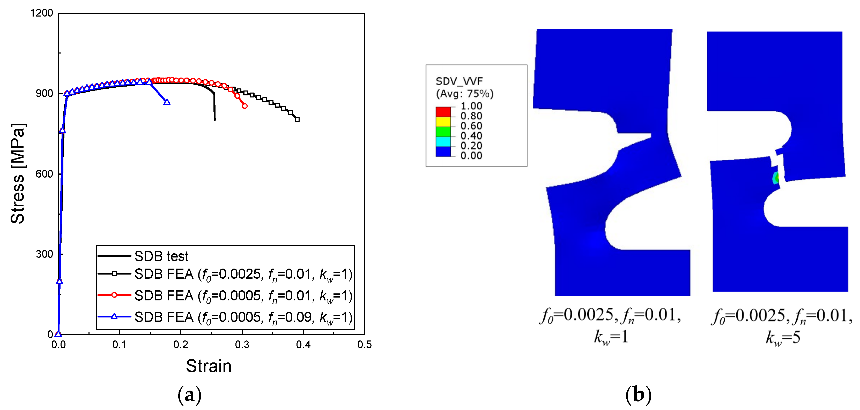
For void nucleation, the three following parameters are involved: the possible nucleated VVF ($f_N$), the average equivalent plastic strain (${\epsilon }_N$), and the standard deviation of the nucleation strain ($s_N$). To simplify parameter calibration, ${\epsilon }_N$ and $s_N$ were determined as 0.3 and 0.1, according to relevant studies [33]. Thus, only $f_0$, $k_w$, and $f_N$ needed to be determined for the shear-modified GTN model. These three parameters not only affect the stress–strain curve, but also influence the specific failure location of the specimen, as shown in Figure 8. It can be observed that, since $f_0$ is correlated with both $f_c$ and $f_F$, a larger $f_0$ obtained greater fracture strain, with all other parameters being equal. Furthermore, increasing the value of $k_w$ shifted the failure mode of specimen NDB90(2) from tension-dominated to shear-dominated, as illustrated in Figure 8b.

Due to the strong nonlinear influence of these three parameters on fracture strain, this study first obtained fracture strain values for various specimens under different parameter combinations through FEA. Subsequently, a surrogate model for fracture strain prediction was established using a BP neural network. Building on this foundation, the optimal values for $f_0$, $k_w$, and $f_N$ could be determined by coupling the model with a GA. The overall framework is shown in Figure 9. According to related research papers [7,33,34], the value ranges of the three parameters are shown in

Table 2. Value range for parameters of $f_0$, $f_N$, and $k_w$.

Parameter	${\mathit{f}}_0$	${\mathit{f}}_{\mathit{N}}$	${\mathit{k}}_{\mathit{w}}$
Range	0.0005–0.005	0.01–0.09	1–5

. Meanwhile, considering optimization efficiency and the stress state of specimens, three specimens—NDB0, SDB, and NDB90(2)—were selected to establish the surrogate models and optimize the model parameters. These specimens correspond to high, medium, and low levels of triaxial stress states, respectively.

To construct the surrogate model, 25 sets of parameters were generated using Latin Hypercube Sampling (LHS) [45] within the parameter ranges. The fracture strains corresponding to each set of $f_0$, $f_N$, and $k_w$ were calculated based on FEA with a shear-modified GTN model. Three BP neural networks corresponding to three specimens were constructed. The networks adopted the 3-5-1 architecture: three input neurons (corresponding to the three parameters $f_0$, $f_N$, and $k_w$), five neurons in a single hidden layer, and one output neuron that predicts the fracture strain. The hidden layer employs hyperbolic tangent activation functions, while the output layer uses a linear activation function. The training process used the Levenberg–Marquardt back propagation algorithm. The networks were trained for a maximum of 1000 epochs with a learning rate of 0.01, and the training stopped automatically if the validation loss did not improve for 20 consecutive iterations. To rigorously evaluate model performance, the dataset was randomly split into training and validation subsets in an 80%:20% ratio. The correlation analysis for these three networks showed correlation coefficients of 0.97, 0.97 and 0.96, respectively, with all root mean square error (RMSE) values below 0.002, which validates that these modes can be effectively used for subsequent parameter calibration.

After establishing the BP surrogate model, the subsequent task involved determining the three parameters in the shear-modified GTN model. This parameter identification process can be mathematically formulated as an optimization problem based on a GA, expressed as follows:

$$\begin{gathered} \mathrm{Find} f_0, f_N, k_w \\ \mathit{Minimize} F(x)={({\epsilon }_{NDB0}^{BP}-{\epsilon }_{NDB0}^{Test})}^2+{({\epsilon }_{SDB}^{BP}-{\epsilon }_{SDB}^{Test})}^2+{({\epsilon }_{NDB90}^{BP}-{\epsilon }_{NDB90}^{Test})}^2 \\ \mathit{s.t.} 0.0005\le f_0\le 0.005, 0.01\le f_N\le 0.09, 1\le k_w\le 5 \end{gathered}$$

(11)

where F(x) is the fitness function; ${\epsilon }_{NDB0}^{BP}$, ${\epsilon }_{SDB}^{BP}$, and ${\epsilon }_{NDB90}^{BP}$ are the values of fracture strain for NDB0, SDB, and NDB90(2) specimens predicted by BP surrogate models; ${\epsilon }_{NDB0}^{Test}$, ${\epsilon }_{SDB}^{Test}$, and ${\epsilon }_{NDB90}^{Test}$ are the values of fracture strain for NDB0, SDB, and NDB90(2) specimens obtained from test. The GA was configured with a population size of 100 and a maximum of 200 generations. The crossover fraction was set to 0.8. The optimization process was set to terminate when the average change in the fitness value was less than 1 × 10⁻⁶ over consecutive generations. The flowchart to determine the parameters by GA is shown in Figure 9, and the final calibrated parameters are shown in

Table 3. Calibrated parameters in shear-modified GTN model.

Parameter	${\mathit{q}}_1$	${\mathit{q}}_2$	${\mathit{f}}_0$	${\mathit{f}}_{\mathit{c}}$	${\mathit{f}}_{\mathit{F}}$	${\mathit{f}}_{\mathit{N}}$	${\mathsf{\epsilon }}_{\mathit{N}}$	${\mathit{s}}_{\mathit{N}}$	${\mathit{k}}_{\mathit{w}}$
value	1	1.5	0.0032	0.044	0.156	0.383	0.3	0.1	3.25

.

4.3. FEA Results and Discussions

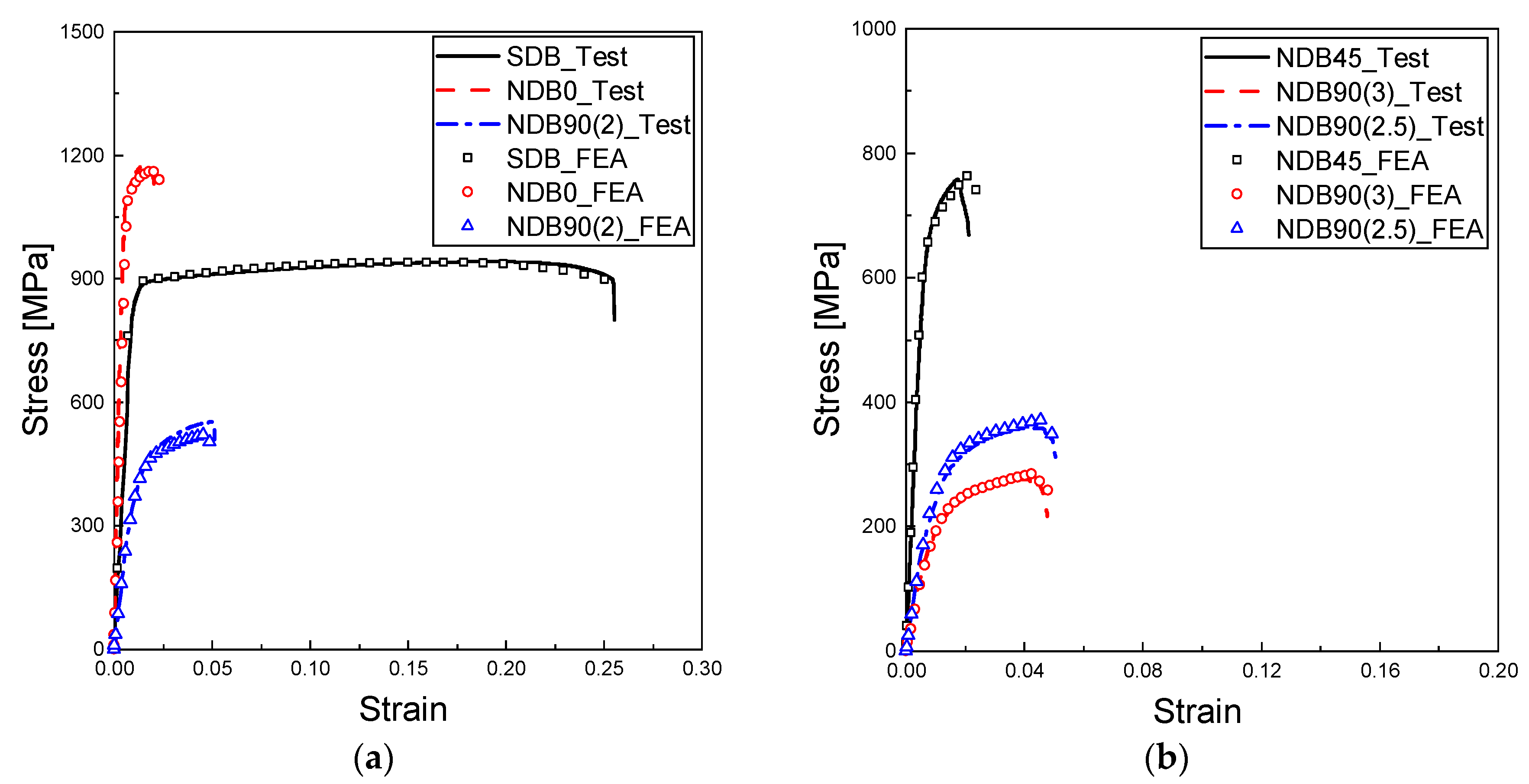
The parameters listed in Table 3 were applied to the FEA to simulate the fracture behavior of these specimens. The fracture strain determined from BP surrogate models and FEA are given in

Table 4. Comparison of fracture strains from BP surrogate and FEA.

Specimen	Surrogate-Predicted Strain	FEA-Predicted Strain	Error (%)
SDB	0.2510	0.250	0.4
NDB0	0.0226	0.0230	1.8
NDB90(2)	0.0491	0.0486	1.0

. It can be seen that the fracture strain values obtained from the surrogate models are essentially consistent with those from FEA, further validating the effectiveness of the surrogate models. The stress–strain curves for NDB0, SDB, and NDB90(2) specimens determined from the FEA are compared to those obtained from tensile tests, as shown in Figure 10a. It can be observed that the stress–strain curves from FEA generally agree with the experimental curves. Furthermore, these same parameters were also used to simulate specimens NDB45, NDB90(2.5), and NDB90(3). Figure 10b presents a comparison of the corresponding stress–strain curves with experimental results, which also demonstrates good agreement. To quantitatively evaluate the prediction accuracy of FEA, the fracture strains obtained from the test and simulations are compared in

Table 5. Comparison of fracture strains from test and FEA.

Specimen	Mean Experimental Strain (±STD)	FEA-Predicted Strain	Error (%)
SDB	0.2522 ± 0.0034	0.250	0.8
NDB0	0.0212 ± 0.0010	0.0230	8.5
NDB90(2)	0.0521 ± 0.0007	0.0486	6.7
NDB45	0.0217 ± 0.0006	0.0238	9.7
NDB90(2.5)	0.0505 ± 0.0002	0.0484	4.2
NDB90(3)	0.0471 ± 0.0006	0.0478	1.5

. The maximum error between the simulated and experimental values is 9.7%. Considering the inherent scatter in the experimental data, it can be concluded that the simulation results are in good agreement with the experimental measurements.

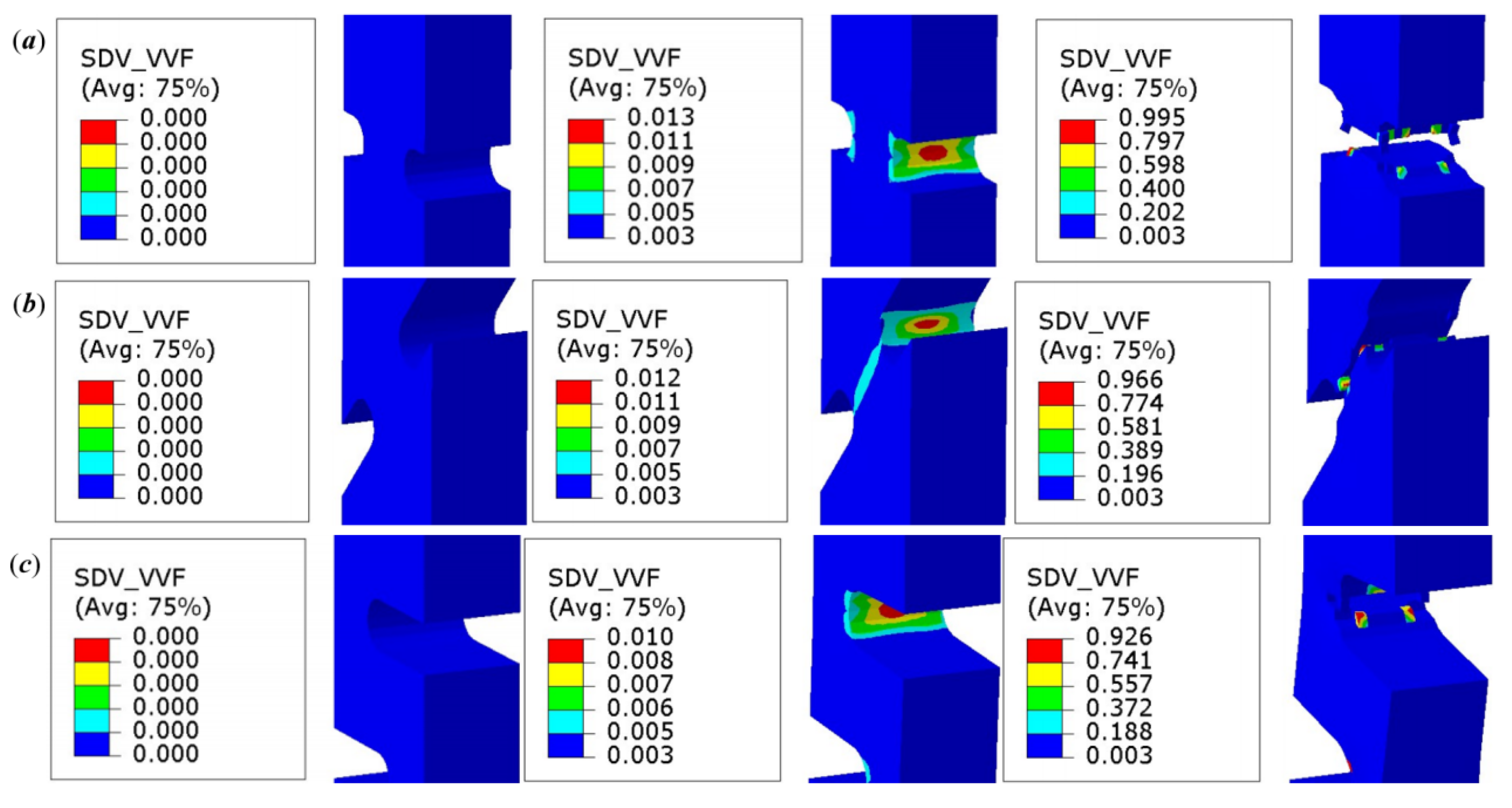
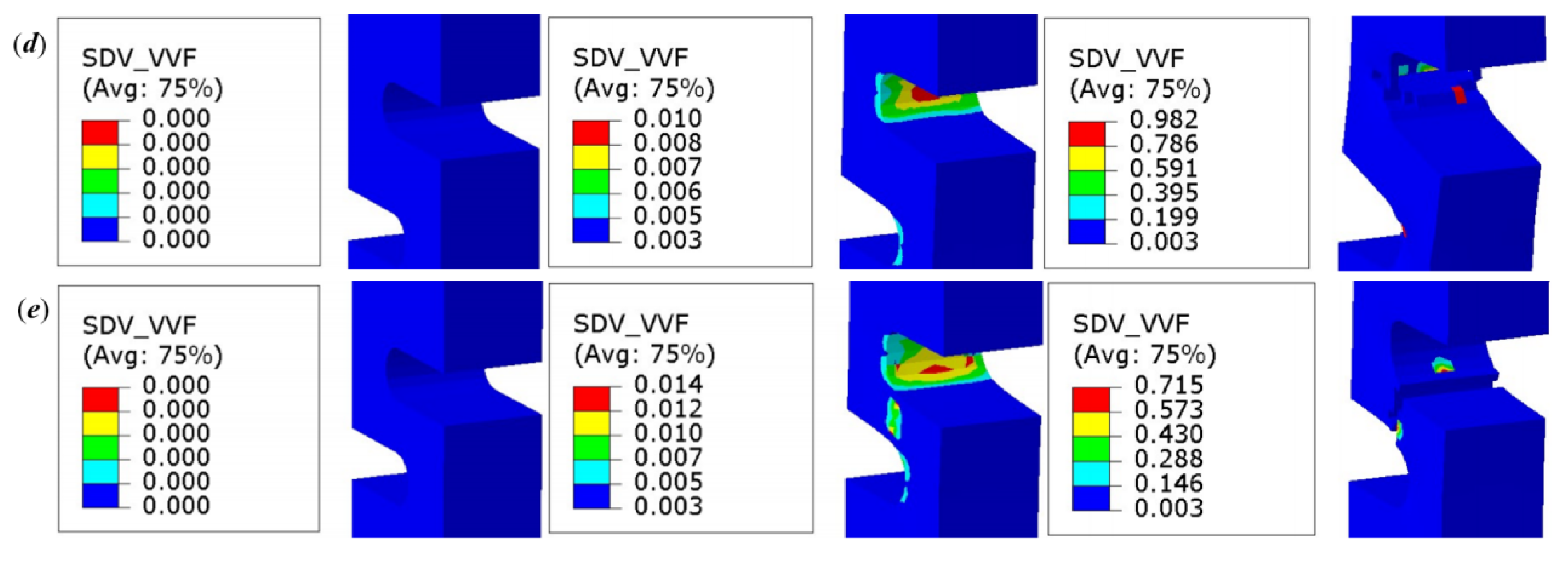
Figure 11 shows the void growth process within each specimen during tensile loading. It can be observed that, due to stress concentration at the notches, voids initially nucleate at these stress concentration points and subsequently propagate inwards through the specimen. It is important to note that, for the three specimens NDB90(2), NDB90(2.5), and NDB90(3), the location of void concentration shifts significantly due to differences in their cross-sectional areas between notches. For specimens NDB90(2.5) and NDB90(3), which are shown in Figure 11c,d and have larger notch spacings, the void growth induced by shear stress in the mid-section is less significant compared to the void growth in the sides under tensile stress. Consequently, failure occurs at the sides. In contrast, for the NDB90(2) specimen, which is shown in Figure 11e and has a smaller notch spacing, the shear-induced void growth in the mid-section is more significant relative to the tensile stress-induced growth in the sides, leading to failure occurring in the middle. This failure location behavior is consistent with the experimental observations for these three specimens, as displayed in Figure 12. This demonstrates that this set of parameters can not only effectively predict the stress–strain curves, but also distinguish failure modes and determine the specific failure locations.

5. Conclusions

This study employed a shear-modified GTN model to simulate the failure behavior of titanium alloy under various stress states. Some model parameters were referenced from the literature, while the remaining three parameters were calibrated using machine learning. Based on the aforementioned studies, the following conclusions can be drawn:

(1)

Tensile tests were performed on specimens featuring various notch geometries to investigate their failure characteristics under different stress states. Specifically, within the NDB90 series, modifications to the cross-sectional area demonstrated two dominant failure mechanisms: tensile-dominated fracture at the notch sides, and shear-dominated failure at the center. These provide the experimental foundation for establishing the shear-modified GTN model and validating its efficacy.

(2)

The shear-modified GTN model involves multiple parameters requiring determination. In this study, the quantitative relationships between $f_0$, $f_c$, and $f_F$ were adopted, while the probability parameters governing void nucleation were established based on the relevant literature. The remaining parameters $f_0$, $f_N$, and $k_w$ were determined using a machine learning approach. FEA results obtained under various parameter combinations were utilized to construct a surrogate model via a BP neural network. Subsequently, an optimal combination of $f_0$, $f_N$, and $k_w$ was identified using a GA method.

(3)

FEA was performed on these specimens to simulate their failure behavior using the optimal parameters determined via machine learning. The fracture strain obtained from FEA for each specimen exhibited a maximum error of less than 10% when compared to the mean fracture strain measured experimentally. Furthermore, the stress–strain curves determined by FEA showed substantial agreement with those obtained from the tests. Additionally, the model effectively differentiated between failure modes and accurately predicted the fracture locations within the NDB90 specimen series. These results validate the efficacy of the proposed model in predicting the failure of Ti6Al4V titanium alloy structures under complex stress states. It should be noted, however, that the generalizability of the shear-modified GTN model and the identified parameters to other material systems has not been verified and may require further investigation and model adaptation. Nevertheless, the current model demonstrates strong potential for critical applications involving titanium components across aerospace, mechanical engineering, and marine structures.

References

1. Wu, X.; Lu, Y.; Wang, M.; Wen, M.; Fu, L.; Ma, S.; Shan, A. Comparative Study the Effect of β-Phase Ratio on Mechanical Properties of Ti-4Al-2.5V-1.5Fe and Ti-6Al-4V Alloys by Heavy Warm Rolling Followed by Annealing. J. Alloys Compd. 2025, 1033, 181274. [Google Scholar] [CrossRef]
2. Seo, S.; Jung, M.; Park, J. Microstructure Control for Enhancing the Combination of Strength and Elongation in Ti-6Al-4V through Heat Treatment. Metals 2024, 14, 985. [Google Scholar] [CrossRef]
3. Xiong, Y.; Duan, W. Predictive Capability Evaluation of Micrograph-Driven Deep Learning for Ti6Al4V Alloy Tensile Strength under Varied Preprocessing Strategies. Metals 2025, 15, 586. [Google Scholar] [CrossRef]
4. Čolić, K.; Kostić, S.M.; Sedmak, S.; Gubeljak, N.; Grbović, A. Structural Integrity and Life Assessment of Ti-6Al-4V Orthopaedic Implants. Metals 2025, 15, 333. [Google Scholar] [CrossRef]
5. Zhang, T.; Lu, K.; Zhang, Z.; Shang, X.; Wang, Q. Experimental Investigations on Parameter Identification and Failure Predictions of Titanium Alloy by Gurson–Tvergaard–Needleman Model. Theor. Appl. Fract. Mech. 2023, 127, 104058. [Google Scholar] [CrossRef]
6. Kim, S.; Kam, D.-H.; Lee, K.-A. Characterization of the Microstructure and Mechanical Properties of Ti-6Al-4V Alloy Fabricated by Wire-Arc Additive Manufacturing: Insights into Fracture Behavior and Strengthening Mechanism. Mater. Sci. Eng. A 2025, 939, 148399. [Google Scholar] [CrossRef]
7. Yang, X.; Li, Y.; Jiang, W.; Duan, M.; Chen, D.; Li, B. Ductile Fracture Prediction of Additive Manufactured Ti6Al4V Alloy Based on an Extended GTN Damage Model. Eng. Fract. Mech. 2021, 256, 107989. [Google Scholar] [CrossRef]
8. Dhar, S.; Dixit, P.M.; Sethuraman, R. A Continuum Damage Mechanics Model for Ductile Fracture. Int. J. Press. Vessels Pip. 2000, 77, 335–344. [Google Scholar] [CrossRef]
9. Chaboche, J.L. Continuum Damage Mechanics: Part I—General Concepts. J. Appl. Mech. 1988, 55, 59–64. [Google Scholar] [CrossRef]
10. Chaboche, J.L. Continuum Damage Mechanics: Part II—Damage Growth, Crack Initiation, and Crack Growth. J. Appl. Mech. 1988, 55, 65–72. [Google Scholar] [CrossRef]
11. Lemaitre, J. A Continuous Damage Mechanics Model for Ductile Fracture. J. Eng. Mater. Technol. 1985, 107, 83–89. [Google Scholar] [CrossRef]
12. Tvergaard, V.; Needleman, A. Analysis of the Cup-Cone Fracture in a Round Tensile Bar. Acta Metall. 1984, 32, 157–169. [Google Scholar] [CrossRef]
13. Tvergaard, V. Influence of Voids on Shear Band Instabilities under Plane Strain Conditions. Int. J. Fract. 1981, 17, 389–407. [Google Scholar] [CrossRef]
14. Yan, R.; Xin, H.; Veljkovic, M. Ductile Fracture Simulation of Cold-Formed High Strength Steel Using GTN Damage Model. J. Constr. Steel Res. 2021, 184, 106832. [Google Scholar] [CrossRef]
15. Kanvinde, A.M.; Deierlein, G.G. The Void Growth Model and the Stress Modified Critical Strain Model to Predict Ductile Fracture in Structural Steels. J. Struct. Eng. 2006, 132, 1907–1918. [Google Scholar] [CrossRef]
16. Yu, F.; Hendry, M.T.; Jar, P.-Y.B.; Li, S.; Li, Z. A Coupled Stress-Triaxiality-Dependent Damage Viscoplasticity Model on Crack Initiation and Propagation in High-Strength Rail Steel. Theor. Appl. Fract. Mech. 2020, 109, 102769. [Google Scholar] [CrossRef]
17. Wang, H.; Shen, T.; Yu, F.; Zheng, R. Ductile Fracture of Hydrostatic-stress-insensitive Metals Using a Coupled Damage-plasticity Model. Fatigue Fract. Eng. Mater. Struct. 2021, 44, 967–982. [Google Scholar] [CrossRef]
18. Gonçalves, P.T.; Arteiro, A.; Rocha, N. End-to-End Simulation of Linerless Composite Pressure Vessels Using 3D Continuum Damage Models. J. Compos. Sci. 2024, 8, 504. [Google Scholar] [CrossRef]
19. Bonora, N. A Nonlinear CDM Model for Ductile Failure. Eng. Fract. Mech. 1997, 58, 11–28. [Google Scholar] [CrossRef]
20. Fang, B.; Lu, A.; Sun, J.; Li, X.; Shen, T. The Simulation of Extremely Low Cycle Fatigue Fracture Behavior for Pipeline Steel (X70) Based on Continuum Damage Model. Metals 2023, 13, 1238. [Google Scholar] [CrossRef]
21. Kachanov, L.M. Rupture Time under Creep Conditions. Int. J. Fract. 1999, 97, 11–18. [Google Scholar] [CrossRef]
22. Zhang, Y.; Zheng, J.; Shen, F.; Li, D.; Münstermann, S.; Han, W.; Huang, S.; Li, T. Ductile Fracture Prediction of HPDC Aluminum Alloy Based on a Shear-Modified GTN Damage Model. Eng. Fract. Mech. 2023, 291, 109541. [Google Scholar] [CrossRef]
23. Li, Y.; Sun, X.; Hu, X.; Cheng, Y.; Xue, F. Uncoupled Ductile Fracture Initiation Model for 5052 Aluminum Alloy with Machine Learning Assisted Identification of the Material Parameters. Eng. Fract. Mech. 2025, 320, 111090. [Google Scholar] [CrossRef]
24. Peng, Z.; Zhao, H.; Li, X. New Ductile Fracture Model for Fracture Prediction Ranging from Negative to High Stress Triaxiality. Int. J. Plast. 2021, 145, 103057. [Google Scholar] [CrossRef]
25. Wei, M.; Lai, X.; Cheng, S.; Ye, X.; Gang, T.; Chen, L. The Extended GTN Model for Stiffness Degradation Prediction Based on Voids Evolution Mechanism. Mater. Today Commun. 2025, 45, 112361. [Google Scholar] [CrossRef]
26. Min, F.; Gao, K.; Zhang, X.; Wei, W.; Qi, P.; Wu, X.; Wen, S.; Huang, H.; Nie, Z.; Zhou, D. A Shear Modified GTN Model Based on Stress Degradation Method for Predicting Ductile Fracture. Model. Simul. Mater. Sci. Eng. 2023, 31, 85004. [Google Scholar] [CrossRef]
27. Malcher, L.; Andrade Pires, F.M.; César De Sá, J.M.A. An Extended GTN Model for Ductile Fracture under High and Low Stress Triaxiality. Int. J. Plast. 2014, 54, 193–228. [Google Scholar] [CrossRef]
28. Min, F.; Gao, K.; Huang, H.; Wen, S.; Wu, X.; Nie, Z.; Zhou, D.; Gao, X. Application of the Modified GTN Model in Predicting Taylor Impact Fracture of 7XXX Aluminum Alloy. Comput. Struct. 2024, 301, 107457. [Google Scholar] [CrossRef]
29. Peng, Z.; Zhao, H.; Li, X.; Yuan, L.; Zhu, T. Ductile Fracture of X80 Pipeline Steel over a Wide Range of Stress Triaxialities and Lode Angles. Eng. Fract. Mech. 2023, 289, 109470. [Google Scholar] [CrossRef]
30. Zhang, K.; Badreddine, H.; Saanouni, K. Ductile Fracture Prediction Using Enhanced CDM Model with Lode Angle-Dependency for Titanium Alloy Ti-6Al-4V at Room Temperature. J. Mater. Process. Technol. 2020, 277, 116462. [Google Scholar] [CrossRef]
31. Nahshon, K.; Hutchinson, J.W. Modification of the Gurson Model for Shear Failure. Eur. J. Mech. A. Solids 2008, 27, 1–17. [Google Scholar] [CrossRef]
32. Xue, L. Constitutive Modeling of Void Shearing Effect in Ductile Fracture of Porous Materials. Eng. Fract. Mech. 2008, 75, 3343–3366. [Google Scholar] [CrossRef]
33. Zhai, Q.; Tang, R.; Liu, Z.; Zhu, P. A Novel Method for Predicting Mechanical Properties of Megacasting Alloy Based on the Modified GTN Model and Machine Learning. Eng. Fail. Anal. 2025, 174, 109536. [Google Scholar] [CrossRef]
34. Ding, X.; Wei, X.; Zhang, X.; Hou, Y.; Zhao, F. Ductile Fracture Prediction of Titanium Foil Based on Shear-Modified GTN Damage Model Considering Size Effect. Eng. Fract. Mech. 2025, 323, 111200. [Google Scholar] [CrossRef]
35. Tian, H.; Zhao, J.; Zhao, R.; He, W.; Meng, B.; Wan, M. The Modified GTN Model for Fracture of Nickel-Based Superalloys Considering Size Effect and Healing Effect in Pulsed Current Assisted Deformation. Int. J. Plast. 2023, 167, 103656. [Google Scholar] [CrossRef]
36. Yildiz, R.A.; Yilmaz, S. Experimental Investigation of GTN Model Parameters of 6061 al Alloy. Eur. J. Mech. A. Solids 2020, 83, 104040. [Google Scholar] [CrossRef]
37. Gholipour, H.; Biglari, F.R.; Nikbin, K. Experimental and Numerical Investigation of Ductile Fracture Using GTN Damage Model on In-Situ Tensile Tests. Int. J. Mech. Sci. 2019, 164, 105170. [Google Scholar] [CrossRef]
38. Cao, T.-S.; Maire, E.; Verdu, C.; Bobadilla, C.; Lasne, P.; Montmitonnet, P.; Bouchard, P.-O. Characterization of Ductile Damage for a High Carbon Steel Using 3D X-Ray Micro-Tomography and Mechanical Tests—Application to the Identification of a Shear Modified GTN Model. Comput. Mater. Sci. 2014, 84, 175–187. [Google Scholar] [CrossRef]
39. Chen, D.; Li, Y.; Yang, X.; Jiang, W.; Guan, L. Efficient Parameters Identification of a Modified GTN Model of Ductile Fracture Using Machine Learning. Eng. Fract. Mech. 2021, 245, 107535. [Google Scholar] [CrossRef]
40. Zhang, T.; Shuai, Y.; Wang, H.; Wang, J.; Lv, Z.; Zhang, Y.; Tian, Y.; Shuai, J.; Zhang, L. An Efficient Method for Determining the Constitutive Relationships of Pipeline Girth Welded Joints Based on Micro-Area Material Testing and Machine Learning. Int. J. Press. Vessels Pip. 2025, 217, 105570. [Google Scholar] [CrossRef]
41. Lu, S.; Zhang, X.; Hu, Y.; Chu, J.; Kan, Q.; Kang, G. Machine Learning-Based Constitutive Parameter Identification for Crystal Plasticity Models. Mech. Mater. 2025, 203, 105263. [Google Scholar] [CrossRef]
42. Marques, A.E.; Parreira, T.G.; Pereira, A.F.G.; Ribeiro, B.M.; Prates, P.A. Machine Learning Applications in Sheet Metal Constitutive Modelling: A Review. Int. J. Solids Struct. 2024, 303, 113024. [Google Scholar] [CrossRef]
43. Benseddiq, N.; Imad, A. A Ductile Fracture Analysis Using a Local Damage Model. Int. J. Press. Vessels Pip. 2008, 85, 219–227. [Google Scholar] [CrossRef]
44. Zhang, Z.L.; Thaulow, C.; Èdegard, J. A Complete Gurson Model Approach for Ductile Fracture. Eng. Fract. Mech. 2000, 67, 155–168. [Google Scholar] [CrossRef]
45. Zhou, Y.; Shen, T.; Du, J. Simulation Analysis and Optimization Design of Dome Structure in Filament Wound Composite Shells. Polymers 2025, 17, 1421. [Google Scholar] [CrossRef]
Figure 1. (a) Schematic representation of the process of nucleation, growth, and coalescence of micro voids, as well as the relationship with the macroscopic load; (b) the deformed configuration of void under shear stress. Reprinted with permission from ref. [27]. Copyright 2025 Elsevier.
Metals 15 00995 g001
Figure 2. (a) A 3D view of damage in the controlled volume at the specimen center at different strain levels; (b) inclusion and elongated cavities obtained with the ID19 beamline observation. Reprinted with permission from ref. [38]. Copyright 2025 Elsevier.
Metals 15 00995 g002
Figure 3. Geometries of the smooth dog bone (SDB) and notched dog bone (NDB) specimens with various notch geometries (unit: mm)): (a) SDB; (b) NDB0; (c) NDB45; (d) NDB90(3); (e) NDB90(2.5); and (f) NDB90(2).
Metals 15 00995 g003
Figure 4. Stress–strain curves obtained from the tensile tests: (a) engineering stress–strain curves of SDB specimen; (b) True stress–plastic strain curves of SDB specimens fitted by Voce hardening model; (c) load–displacement curves of NDB specimens with various notch geometries; and (d) average stress–strain curves of NDB specimens with various notch geometries.
Metals 15 00995 g004
Figure 5. Pictures of specimens after tensile tests: (a) SDB; (b) NDB0; (c) NDB45; (d) NDB90(3); (e) NDB90(2.5); and (f) NDB90(2).
Metals 15 00995 g005
Figure 6. Failure locations for NDB specimens with various notch spacings: (a) NDB90(3); (b) NDB90(2.5); and (c) NDB90(2).
Metals 15 00995 g006
Figure 7. FEA models for SDB and NDB specimens.
Metals 15 00995 g007
Figure 8. FEA results with various parameter values in shear-modified GTN model: (a) FEA results for stress–strain curves; (b) FEA results for failure locations.
Metals 15 00995 g008
Figure 9. Framework for calculation of parameters of f 0 , f N , and k w based on BP neural network and GA.
Metals 15 00995 g009
Figure 10. Comparisons of stress–strain curves from test and FEA: (a) SDB, NDB0, and NDB90(2) specimens; (b) NDB45, NDB90(3), and NDB90(2.5) specimens.
Metals 15 00995 g010
Figure 11. Void growth in NDB specimens: (a) NDB0 specimen; (b) NDB45 specimen; (c) NDB90(3) specimen; (d) NDB90(2.5) specimen; and (e) NDB90(2) specimen.
Metals 15 00995 g011aMetals 15 00995 g011b
Figure 12. Comparison of failure locations in FEA and tests: (a) NDB90(3) specimen; (b) NDB90(2.5) specimen; and (c) NDB90(2) specimen.
Metals 15 00995 g012