Optimization of L-PBF Process Parameters: A Multi-Objective Framework for Variance Reduction and Mechanical Strength Enhancement Using Linear Programming and Multi-Objective Methods

Abstract

A new approach to the multi-criteria optimization of L-PBF process parameters in the face of high variability is proposed, based on the application of the reward function (RF), which is essentially the inverse of the Taguchi quality loss function (QLF). The RF is defined as the logarithm of the ratio of the design parameter value to the minimum target parameter value. For values below 1, the RF becomes sharply negative. Logarithmic additivity enables the optimization of the target function to be defined as a sum of reward functions for the optimization criteria, each with a corresponding weight coefficient. This makes it possible to formulate the optimization problem in terms of linear programming. This approach was tested in the optimization of the L-PBF technological modes of AISI 321 powder, leading to a 6.7% increase in productivity. The mechanical properties of the samples obtained were not inferior to those of the alloyed samples using the previously recommended process parameters in terms of ultimate strength, and they exceeded the latter by 5% in terms of conditional yield strength. Process variability significantly decreased; the RMS of ultimate strength decreased nine-fold, conditional yield strength decreased ten-fold, and relative elongation decreased two-fold.

1. Introduction

Laser powder bed fusion (L-PBF) is an additive manufacturing technique that employs high-power lasers to melt metallic powders into three-dimensional objects [1]. The quality of L-PBF parts is affected by various process parameters, including laser power (P), scanning speed (V), hatch spacing (h), and layer thickness (t) [2,3]. These parameters can be combined into a single indicator known as volume energy density (EV) [4]:

$$EV={\displaystyle \frac{P}{V·h·t}}$$

(1)

Microstructural defects, such as gas and lack-of-fusion pores, significantly influence the mechanical properties of L-PBF parts [2,5]. While optimizing parameters can reduce porosity, achieving the desired microstructure, strength, and ductility simultaneously remains challenging [5,6,7]. Additionally, reducing porosity may slow production speed [5,8].

The quality of L-PBF materials is determined by both porosity and mechanical properties, including yield strength (σ0.2), ultimate tensile strength (σv), and elongation at break (δ). Optimizing these characteristics often requires trade-offs due to the varying importance of product requirements. Furthermore, the relationship between mechanical properties and microstructural defects can be weak or negative [9]. Most studies focus on optimizing a single characteristic, with limited research on simultaneous optimization of multiple properties, presenting a significant challenge [9,10,11,12].

To determine optimal processing parameters, AM models and design-of-experiments (DoE) methods are essential. The literature reveals many studies on design-of-experiments (DoE) methods (e.g., Taguchi, half-factorial, central composite) and analysis of variance (ANOVA) for defining important parameters [13,14,15,16,17,18,19,20,21,22,23,24,25,26,27,28,29,30,31,32,33,34]. Full factorial DoE involves equal replicates for all combinations of processing parameters, allowing precise responses for parameter effects and interactions [13]. However, full factorial DoE can be costly and time-consuming [14], necessitating fractional factorial DoE methods like Taguchi, which efficiently analyzes significant parameter interactions and main effects [15]. Taguchi offers a systematic approach to optimizing designs for quality and cost using orthogonal arrays [16]. The Taguchi method aims to optimize parameters for metal additive manufacturing, particularly directed energy deposition (DED), to reduce deviations and achieve target output values [17,18,19,20,21,22]. Manjunath et al. [18] optimized DED using the Taguchi L9 orthogonal design, achieving optimal interfacial adhesion with Colmonoy 52 alloy. Liu et al. [17] employed the L25 design to maximize density in AlSi10Mg parts by optimizing laser power, scanning speed, powder feed rate, and shielding gas flow. The method has been applied to various materials, including titanium alloys [19,20], nickel-based superalloys [21], and others. Key findings include the important influence of layer thickness and scanning speed on hardness and surface roughness [22] The response surface method (RSM) improves stochastic response values through design-of-experiments (DoE) and regression analysis [23]. Dada et al. [24] used full-factor DoE with RSM for L-PBF high-entropy alloys, while Pant et al. [25] modeled the DED process of 316L stainless steel with RSM. El-Sayed et al. [26] proposed optimal parameters for Ti-6Al-4V medical implants, concluding that higher density reduces surface roughness and porosity. Marmarelis et al. [27] combined Taguchi and RSM to study the effects of processing parameters on AlSi10Mg specimens, identifying hatch spacing as a significant factor.

Grey relational analysis (GRA) is often used alongside Taguchi’s method for multi-response and multifactor experiments. When an optimization problem involves multiple conflicting criteria, GRA can help to prioritize and weigh these criteria in order to find a balanced solution [28,29,30].

The impact of factors (independent parameters) on quality indicators is multidirectional. Therefore, the problem of optimizing technological modes is multifactorial and multi-criteria [31]. One method for solving such an optimization problem is linear programming. The idea behind this method is that, in order to reduce the dimensionality of the problem, a target function is formed from a linear combination of the optimization criteria. Furthermore, a constraint matrix consisting of inequalities is formed, including these criteria and the optimization parameters [32]. The linear programming method, due to its specificity—and linearity—shows good results near the vector of optimal process parameters. Accordingly, its efficiency depends on the type of target function that includes the required optimization criteria, i.e., the target design parameters or, in other words, its quality characteristics. The present study aims to develop a linear programming method for optimizing L-PBF parameters and justify the type of target function that is resistant to variation in the factors affecting the criteria. To this end, Taguchi’s approach is supposed to be used.

The variability of additive manufacturing is due to the significant number of factors that influence growing conditions, which results in a decrease in the quality of parts.

Taguchi pointed out that excessive variation in quality indicators is the root cause of poor quality. In other words, he emphasized the importance of reducing process variability relative to design parameters and of bringing the average values of process parameters to target values [33,34]. A quality loss function is used to quantify the quality loss, which depends on the mean square deviation $\sigma$ and the deviation of the product characteristic ${\overline{x}}_i$ from the target value ${\overline{x}}_{i0}$:

$$QLF=C_i({({\overline{x}}_i-{\overline{x}}_{i0})}^2+{\sigma }_i^2),$$

(2)

where ${\overline{x}}_i-{\overline{x}}_{i0}$ is the difference between average and target value; $\sigma$ is the variation characteristic, i.e., noise; $\mathrm{a}\mathrm{n}\mathrm{d}{C}_i$ is the quality loss impact factor.

Taguchi suggests that reducing the variation in product characteristics relative to their mean values will reduce quality losses. This reduction in variation is achieved by adjusting the mean value relative to the target value using a correction factor:

$$S/N_i=-10{log}_{10}\left[{\displaystyle \frac{{({\overline{x}}_i-{\overline{x}}_{i0})}^2}{{\sigma }_i^2}}\right]=-10{\mathit{log}}_{10}\left({\displaystyle \frac{QLF/C_i}{{\sigma }_i^2}}-1\right),$$

(3)

where ${\displaystyle \frac{{({\overline{x}}_i-{\overline{x}}_{i0})}^2}{{\sigma }_i^2}}$ is the signal-to-noise ratio indicator.

The signal-to-noise ratio depends on the quality characteristics that need to be optimized during the experiment (see [33]).

(a)

Taguchi used the logarithmic scale in decibels (dB) because this scale is the standard for most acoustic, radio, etc. measurements. It provides a uniform and comprehensible means of expressing and comparing parameter ratios.

(b)

It should also be noted that the logarithmic scale has the property of large negative values when the argument of the function becomes less than 1, which is very convenient when the argument of the logarithmic function is used as a constraint, for example, ${\displaystyle \frac{QLF}{C_i}}<2{\sigma }_i^2$.

In the generalizable target function, the quality characteristics and the process parameters should be represented in dimensionless form. This recommendation can also be referred to as a constraint. In this vein, we can introduce the concept of a safety factor to define the limits of deviations from quality targets. A similar approach is used in our structural analysis, where the margin of safety (MoS or MS) is defined.

The MS is a measure of satisfying design requirements (requirement verification). The margin of safety can be conceptualized to represent how much of the structure’s total capability is held “in reserve” during loading.

$$MS={\displaystyle \frac{designload}{minimumtargetloadfordesign-1}}$$

(4)

MS is a measure of structural capability; this definition of the margin of safetycommonly seen in textbooks [35,36] describes what additional load (beyond the design load) a part can withstand before failing. In effect, it is a measure of excess capability. MS is a measure of requirement verification; any agencies and organizations such as National Aeronautics and Space Administration (NASA) [37] and American Institute of Aeronautics and Astronautics (AIAA) [38] define the margin of safety including the design factor. In other words, the margin of safety is calculated after applying the design factor. In the case of a margin of 0, the part is at exactly the required strength (that is, the safety factor would equal the design factor).

Clearly, the concept of MS as a measure of requirement verification can be extended to any relevant quality characteristic (or design factor).

The present study solves the following problems in such a formulation:

• Development of a framework for multi-criteria optimization of additive manufacturing technological parameters using formalized quality indicators.
• Approval of the developed framework for multi-criteria optimization of technological parameters for L-PBF AISI 321 under conditions of increased variability.

The general strategy of the study is as follows:

Design of experiments (DoE) is performed using the Taguchi plan, with mechanical characteristics and surface roughness as the dependent variables, to identify target process parameters and investigate process variability.

If the Taguchi method cannot identify the target process parameters due to high variability, GRA is used to select one of the process parameters from the DoE results and designate it a target value.

Constraints and a target function are formed using margins of safety and previously obtained target values for design parameters.

The optimal L-PBF parameters are sought using the linear programming method with the target function, and the constraint matrix is formed in terms of the margins of safety.

2. Theoretical Foundations of the Optimization Method and Models

According to the technical requirements for the workpieces, a set of design factors (5) are established. These factors may include tensile strength, surface roughness, residual porosity and other parameters.

$$X_b=\left\{x_{bi}\right\},i=\dots I,$$

(5)

Suppose that, as a result of the technological process, we obtain a workpiece characterized by a set of technological quality parameters.

$$X=\left\{x_i\right\},i=\dots I$$

(6)

Let us apply the concepts of design factor and margin of safety to other quality parameters, as well as to structural analysis. Assuming that the workpiece meets the technical requirements and is therefore considered to be of good quality, the margin of safety for each factor must be greater than 0, in accordance with the following relationship (7):

$$\left.\begin{array}{c}M{S}_i={\displaystyle \frac{x_{ib}-x_i}{x_{ib}}}=1-{\displaystyle \frac{x_i}{x_{ib}}},\mathrm{w}\mathrm{h}\mathrm{e}\mathrm{n}{x}_i\le x_{ib}=x_{\mathrm{m}\mathrm{a}\mathrm{x}}\\ M{S}_i={\displaystyle \frac{x_i-x_{ib}}{x_{ib}}}={\displaystyle \frac{x_i}{x_{ib}}}-1,\mathrm{w}\mathrm{h}\mathrm{e}\mathrm{n}{x}_i\ge x_{ib}=x_{\mathrm{m}\mathrm{i}\mathrm{n}}\end{array}\right\}$$

(7)

Next, based on Taguchi’s approach, we introduce the reward function (RF), which is essentially the opposite of QLF and should increase if the margin of safety increases.

Using the property of the logarithmic function to decrease sharply at values of the argument less than 1, RF can be represented as a value proportional to the logarithm of MS + 1.

$$M{S}_i^1=M{S}_i+1={\left({\displaystyle \frac{designvalue}{mintargetfordesignvalue}}\right)}_i$$

(8)

$$R{F}_i=K_i+k_i\mathrm{l}\mathrm{n}\left(M{S}_i^1\right),$$

(9)

$k_i$ is the coefficient of influence of the i-th quality parameter, and $M{S}_i^1$ is the offset margin of safety.

When $M{S}_i^1=1$, $R{F}_i$ also takes on a nominal value of K_i, and k_i is the influence coefficient of the i-th quality characteristic.

Analysis of (9) shows that as we approach the zero critical value, the reward function decreases sharply due to an increase in process variability.

Based on Equation (1), it is clear that the reward function $R{F}_i$ for the i-th quality parameter depends on laser power (P), scanning speed (V), hatch spacing (h), and layer thickness (t).

$$R{F}_i=F(P/v,h,t)$$

(10)

Let us decompose the functional dependence (10) into a Taylor series with respect to the nominal (‘target’) state $F_0(P_0/v_0,h_0,t_0)$, retaining the first terms of the series. This represents the linear Equation (11) in the parameter plane.

$$\begin{array}{l}{F}_i=F_{0i}(P_0/v_0,h_0,t_0)+{{\displaystyle \frac{\partial F_i}{\partial (P/v)}}}_0\left(P/v-P_0/v_0\right)+{{\displaystyle \frac{\partial F_i}{\partial h}}}_0(h-h_0)+{{\displaystyle \frac{\partial F_i}{\partial t}}}_0(t-t_0)=\\ =F_{0i}+{(k_{P/v})}_i\left({\displaystyle \frac{P/v}{P_0/v_0}}-1\right)+{(k_h)}_i\left({\displaystyle \frac{h}{h_0}}-1\right)+{(k_t)}_i\left({\displaystyle \frac{t}{t_0}}-1\right)\end{array}$$

(11)

The coefficients ${(k_{P/v})}_i,{(k_h)}_i,{(k_t)}_i$ characterize the RF trend in relation to the variation of the factors and determine the inclination angles of the parameter plane (11) to the axes of the dimensionless parameters ${\displaystyle \frac{P/v}{P_0/v_0}},{\displaystyle \frac{h}{h_0}},{\displaystyle \frac{t}{t_0}}$.

Taking dependencies (9)–(11) into account, the reward function for the quality parameter i can be defined as follows:

$$R{F}_i=\ln K_i+{(k_{P/v})}_i\ln \left({\displaystyle \frac{P/v}{P_0/v_0}}\right)+{(k_h)}_i\ln \left({\displaystyle \frac{h}{h_0}}\right)+{(k_t)}_i\ln \left({\displaystyle \frac{t}{t_0}}\right)$$

(12)

In this case, the offset margin of safety for quality indicator i will depend on the following:

$$M{S}_{i\min }^1\le K_i{\left({\displaystyle \frac{P/v}{P_0/v_0}}\right)}^{k_{P/v}}{\left({\displaystyle \frac{h}{h_0}}\right)}^{k_h}{\left({\displaystyle \frac{t}{t_0}}\right)}^{k_t}$$

(13)

Consider the following quality parameters and their limitations.

• an offset margin of safety in terms of performance:

  $$\begin{array}{l}M{S}_{V\min }^1\le \left({\displaystyle \frac{V}{V_{\min }}}\right)=K_V\left({\displaystyle \frac{v}{v_0}}\right)\left({\displaystyle \frac{h}{h_0}}\right)\left({\displaystyle \frac{t}{t_0}}\right),\\ K_V=\left({\displaystyle \frac{V_0}{V_{\min }}}\right)\end{array}$$

  (14)
• with lower limit $V\ge V_{\min }$;
• an offset margin of safety in terms of tensile strength

  $$M{S}_{\sigma \min }^1\le \left({\displaystyle \frac{\sigma }{{\sigma }_{\min }}}\right)=K_{\sigma }{\left({\displaystyle \frac{P/v}{P_0/v_0}}\right)}^{\sigma p}{\left({\displaystyle \frac{h}{h_0}}\right)}^{\sigma h}{\left({\displaystyle \frac{t}{t_0}}\right)}^{\sigma t},K_{\sigma }=\left({\displaystyle \frac{{\sigma }_0}{{\sigma }_{\min }}}\right)$$

  (15)
• with lower limit $\sigma \ge {\sigma }_{\min }$;
• an offset margin of safety in terms of relative elongation

  $$\begin{array}{l}M{S}_{\delta \min }^1\le \left({\displaystyle \frac{\delta }{{\delta }_{\min }}}\right)=K_{\delta }{\left({\displaystyle \frac{P/v}{P_0/v_0}}\right)}^{\delta p}{\left({\displaystyle \frac{h}{h_0}}\right)}^{\delta h}{\left({\displaystyle \frac{t}{t_0}}\right)}^{\delta t},\\ K_{\delta }=\left({\displaystyle \frac{{\delta }_0}{{\delta }_{\min }}}\right)\end{array}$$

  (16)
• with lower limit $\delta \ge {\delta }_{\min }$;
• an offset margin of safety in terms of surface roughness

  $$\begin{array}{l}M{S}_{R\min }^1\le \left(2-{\displaystyle \frac{Rz}{R{z}_{\max }}}\right)=K_{Ra}{\left({\displaystyle \frac{P/v}{P_0/v_0}}\right)}^{Rp}{\left({\displaystyle \frac{h}{h_0}}\right)}^{Rh}{\left({\displaystyle \frac{t}{t_0}}\right)}^{Rt},\\ K_{Rz}=\left(2-{\displaystyle \frac{R{z}_0}{R{z}_{\max }}}\right)\end{array}$$

  (17)
• with upper limit $Rz\le R{z}_{\max }$.

Following the principle of additivity, the total reward function can be expressed as follows:

$$R{F}_{\sum }={\displaystyle \sum _{i=1}^N{C}_i}\cdot R{F}_i$$

(18)

where $C_i$ is the significance coefficient of the i-th quality parameter, which takes a value from 0 to 1 and can be determined by expert judgement depending on the requirements of the workpiece.

Considering (12) to (17), the result dependency (18) is expressed as follows:

$$\begin{array}{l}R{F}_{\sum }=(c_{\sigma }\sigma p+c_{\delta }\delta p+c_{R}Rp)\ln \left({\displaystyle \frac{P}{P_0}}\right)+(c_V-c_{\sigma }\sigma p-c_{\delta }\delta p-c_{R}Rp)\ln \left({\displaystyle \frac{v}{v_0}}\right)+\\ +(c_V+c_{\sigma }\sigma h+c_{\delta }\delta h+c_{R}Rh)\ln \left({\displaystyle \frac{h}{h_0}}\right)+(c_V+c_{\sigma }\sigma t+c_{\delta }\delta t+c_{R}Rt)\ln \left({\displaystyle \frac{t}{t_0}}\right)+\ln \left(K_V{K}_{\sigma }{K}_{\delta }{K}_{Rz}\right)\end{array}$$

(19)

In accordance with the quality management objective, the total reward function should be set up to maximize, as follows:

$$R{F}_{\sum }\to \max$$

(20)

The dependencies from (13) to (17) can be expressed in matrix form by taking the logarithm of the left and right sides of these inequalities, respectively.

$$\begin{array}{l}{RF}_{V\min }=\ln \left(M{S}_{V\min }^1\right)\le \ln (K_V)+\ln \left({\displaystyle \frac{v}{v_0}}\right)+\ln \left({\displaystyle \frac{h}{h_0}}\right)+\ln \left({\displaystyle \frac{t}{t_0}}\right)\\ {RF}_{\sigma \min }=\ln \left(M{S}_{\sigma \min }^1\right)\le \ln (K_{\sigma })+\sigma p\cdot \ln \left({\displaystyle \frac{P/v}{P_0/v_0}}\right)+\sigma h\cdot \ln \left({\displaystyle \frac{h}{h_0}}\right)+\sigma t\cdot \ln \left({\displaystyle \frac{t}{t_0}}\right)\\ {RF}_{\delta \min }=\ln \left(M{S}_{\delta \min }^1\right)\le \ln (K_{\delta })+\delta p\cdot \ln \left({\displaystyle \frac{P/v}{P_0/v_0}}\right)+\delta h\cdot \ln \left({\displaystyle \frac{h}{h_0}}\right)+\delta t\cdot \ln \left({\displaystyle \frac{t}{t_0}}\right)\\ {RF}_{Rz\max }=\ln \left(M{S}_{Rz\max }^1\right)\le \ln (K_{Rz})+Rp\cdot \ln \left({\displaystyle \frac{P/v}{P_0/v_0}}\right)+Rh\cdot \ln \left({\displaystyle \frac{h}{h_0}}\right)+Rt\cdot \ln \left({\displaystyle \frac{t}{t_0}}\right)\end{array}$$

(21)

In this case,

$$A\cdot X\ge B,$$

(22)

where

$$A=\left[\begin{array}{ccccc}0& 1& 1& 1& \ln \left(K_V\right)\\ \sigma p& -\sigma p& \sigma h& \sigma t& \ln \left(K_{\sigma }\right)\\ \delta p& -\delta p& \delta h& \delta t& \ln \left(K_{\delta }\right)\\ Rp& -Rp& Rh& Rt& \ln \left(K_{Rz}\right)\\ 0& 0& 0& 0& 1\end{array}\right]$$

is the matrix of coefficients of influence of technological parameters;

$X={\left[\begin{array}{cccc}\ln \left({\displaystyle \frac{P}{P_0}}\right)& \ln \left({\displaystyle \frac{v}{v_0}}\right)& \ln \left({\displaystyle \frac{h}{h_0}}\right)& \ln \left({\displaystyle \frac{t}{t_0}}\right)\begin{array}{c}1\end{array}\end{array}\right]}^T$ is the vector of variables; and

$B={\left[\begin{array}{cccc}\ln \left(M{S}_{V\min }\right)& \ln \left(M{S}_{\sigma \min }\right)& \ln \left(M{S}_{\delta \min }\right)& \ln \left(M{S}_{Rz\min }\right)\end{array}\right]}^T$ is the constraint vector.

The objective functions (19) and (20) can be expressed in matrix form as follows:

$$\begin{array}{l}R{F}_{\sum }=C\cdot A\cdot X\\ C\cdot A\cdot X\to \max \end{array},$$

(23)

where $C=\left[\begin{array}{ccccc}{c}_V& c_{\sigma }& c_{\delta }& c_R& 0\end{array}\right]$ is the vector of the significance coefficients of quality parameters.

The target function in the form of (23) and the constraints in the form of the inequalities in (22) represent the optimization problem, which is solved using the linear programming method. The dependencies obtained in (22) and (23) are defined in the form of a classical direct linear programming problem, in which the maximum total reward is sought, as the technological parameters vary within (24).

$$\left.\begin{array}{l}\ln (P_{\min }/P_0)\le \ln (P/P_0)\le \ln (P_{\max }/P_0)\\ \ln (v_{\min }/v_0)\le \ln (v/v_0)\le \ln (v_{\max }/v_0)\\ \ln (h_{\min }/h_0)\le \ln (h/h_0)\le \ln (h_{\max }/h_0)\\ \ln (t_{\min }/t_0)\le \ln (t/t_0)\le \ln (t_{\max }/t_0)\end{array}\right\}$$

(24)

Taking (24) and the matrix notation of (22) into account, the latter can be written in the extended form (25):

$$A_{en}\cdot X\ge B_{en},$$

(25)

where the expanded matrices are of the following form:

$$\begin{gathered} A_{en}=\left[\begin{array}{ccccc}0& 1& 1& 1& \ln \left(K_V\right)\\ \sigma p& -\sigma p& \sigma h& \sigma t& \ln \left(K_{\sigma }\right)\\ \delta p& -\delta p& \delta h& \delta t& \ln \left(K_{\delta }\right)\\ Rp& -Rp& Rh& Rt& \ln \left(K_{Rz}\right)\\ 1& 0& 0& 0& 0\\ -1& 0& 0& 0& 0\\ \dots & & & & \\ 0& 0& 0& 1& 0\\ 0& 0& 0& -1& 0\end{array}\right] \\ {B}_{en}=\begin{array}{cccc}[\ln \left(M{S}_{V\min }\right)& \ln \left(M{S}_{\sigma \min }\right)& \ln \left(M{S}_{\delta \min }\right)& \dots \\ \ln \left(M{S}_{Rz\min }\right)& \ln (P_{\max })& -\ln (P_{\min })& \dots {]}^T\end{array} \end{gathered}$$

(26)

Thus, the objective function (23) and inequalities (26) correspond to the formulation of the linear programming optimization problem.

3. Materials and Methods

Experimental Design and Sample Preparation

The influence of variability in metallic powder bed fusion parameters on mechanical properties was investigated using robust experimental design methods in order to obtain optimal values for the technological parameters of the L-PBF process, to minimize variability in mechanical properties, and to maximize productivity.

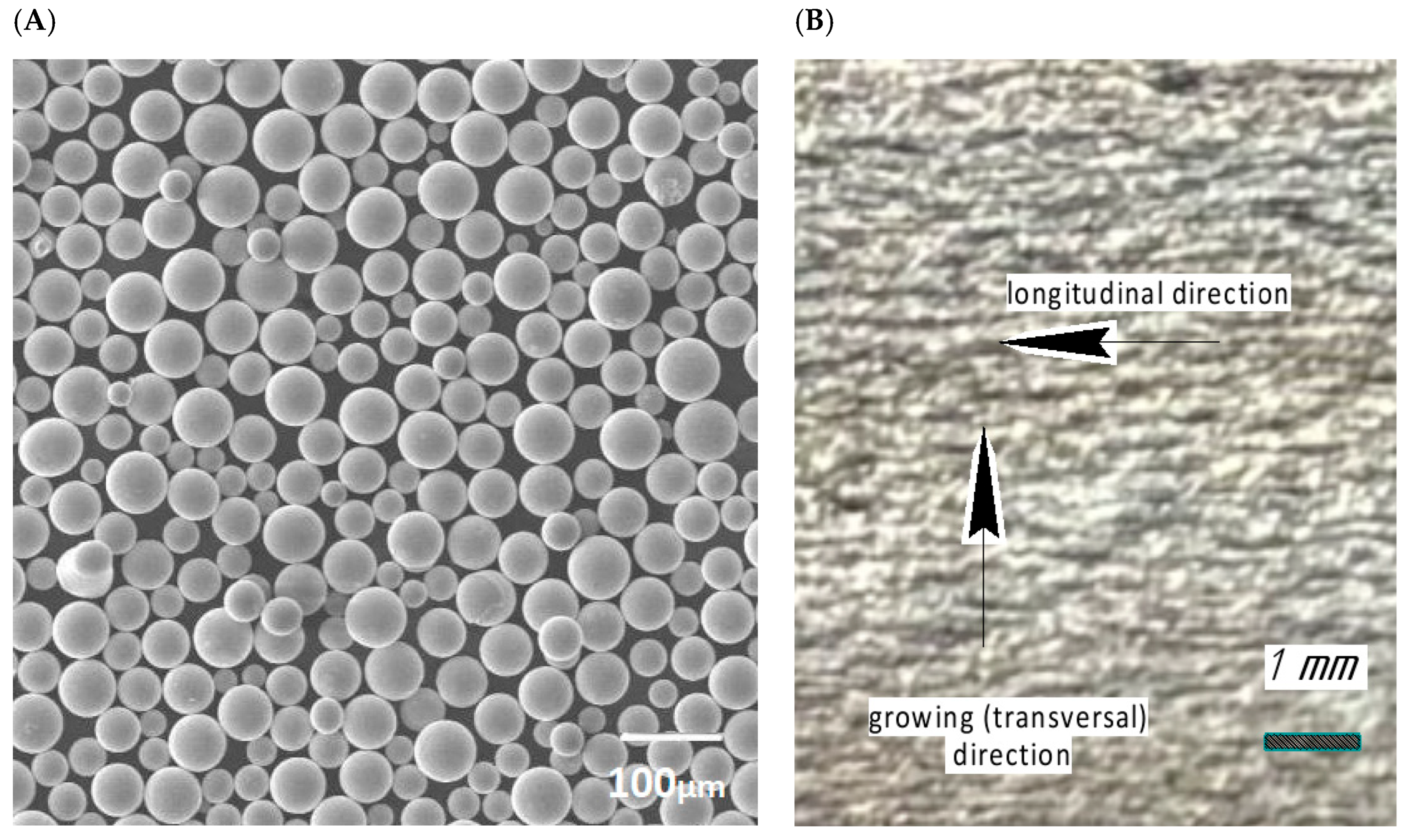
The following process parameters were selected as factors for the study: laser power (P), volume energy density (EV), scanning speed (V), hatch distance (h), and layer thick-ness (t). The basic experimental plan was a Taguchi L9 orthogonal design with three levels of parameter variation. The L9 DOE is presented in

Table 1. Design of L9 orthogonal experiment for four factors.

Experiment No.	Power, W	Scanning Speed, mm/s	Scanning Step, mm	Layer Thickness, mm	Linear Energy Density, W/mm
1	200	750	0.065	0.05	0.267
2	200	800	0.090	0.05	0.250
3	200	850	0.115	0.06	0.235
4	229	750	0.090	0.06	0.305
5	229	800	0.115	0.05	0.286
6	229	850	0.065	0.05	0.269
7	257	750	0.115	0.06	0.343
8	257	800	0.065	0.06	0.321
9	257	850	0.090	0.05	0.302

. Each experiment was re-peated three times. The specimens were manufactured using an 3DLAM Mid 3D printer (3DLAM, St.-Peterburg, Russia) equipped with a laser with a maximum power of 400 W. A metallic powder of a AISI 321 Cr-Ni high alloy steel was used as the feedstock powder material with a granulometric composition of 15–53 µm (Powder size distribution (PSD): D10 = 21.2 μm, D50 = 33.5 μm, D90 = 52.8 μm). The chemical composition of the alloy is given in

Table 2. Chemical composition of AISI 321 Cr-Ni-high alloy steel.

Spectrum	C	Si	Mn	Cr	Ni	Ti	S	P	Fe
wt. %	<0.12	<0.80	<2.00	17.0–19.0	9.0–11.0	5.0–8.0	<0.02	<0.40	base

and the granulo-metric composition in Figure 1A.

The mechanical testing of specimens produced using L-PBF technology was per-formed at room temperature (20 °C) using an Instron 8802 testing machine (Instron, Nor-wood, MA, USA). Flat specimens without heads, measuring 140 mm × 20 mm × 3 mm, were produced in accordance with DIN EN ISO 6892:1998 [39]. The roughness of the grown specimens was measured by Rz (ISO 21920-2:2021 [40]) using a profilometer (Vostok 7 ISHP-210, Vostok-7, Moscow, Russia). Roughness measurements were taken in two directions (Figure 1B): along the 20 mm width of the specimen (longitudinal direction) and along the 140 mm length of the specimen (transversal direction, i.e., in the growing direction).

4. Results

4.1. Evaluating the Variability of Taguchi Experiment Results

The purpose of using Taguchi’s method is to determine the influence of the main effects of the process parameters on quality parameters and, accordingly, to find target values of $P_0/v_0,h_0,t_0$, included in the dependencies for constraints (13)–(17).

The results of the tensile tests and roughness measurements on the specimens (the mean of three specimens for each experimental run) are shown in

Table 3. Tensile and roughness test results.

Experiment No.	Tensile Strength, MPa	Yield Strength, MPa	Relative Elongation, %	Longitudinal Rz, µm	Transversal Rz, µm
1	726	359	51.19	19.70	22.95
2	728	464	54.92	20.84	21.11
3	525	339	20.82	17.42	18.17
4	744	476	55.48	19.78	20.86
5	717	434	57.41	19.23	21.10
6	735	464	55.41	19.42	19.67
7	727	436	56.17	19.63	22.68
8	731	433	57.34	20.70	23.82
9	749	428	53.93	21.17	22.40

.

Table 4. Spearman correlation matrix.

	Layer Thickness, mm	Linear Energy Density, W/mm	Tensile Strength, MPa	Yield Strength, MPa	Relative Elongation, %	Longitudinal Rz, µm	Transversal Rz, µm
Layer thickness, mm	1.000	0.400	−0.372	−0.099	−0.323	−0.327	−0.018
Linear energy density, W/mm	0.400	1.000	0.568	0.419	0.606	0.440	0.693
Tensile strength, MPa	−0.372	0.568	1.000	0.718	0.972	0.824	0.677
Yield strength, MPa	−0.099	0.419	0.718	1.000	0.757	0.574	0.155
Relative elongation, %	−0.323	0.606	0.972	0.757	1.000	0.766	0.668
Rz longitudinal, µm	−0.327	0.440	0.824	0.574	0.766	1.000	0.726
Rz transversal, µm	−0.018	0.693	0.677	0.155	0.668	0.726	1.000

shows the Spearman’s matrix of mutual correlation between the process parameters and the main quality parameters (responses). Analysis of the matrix shows that except for roughness in the transverse direction (with a statistically significant correlation coefficient of r = 0.693 and stable linear energy density), the influence of process parameters on other quality parameters is variable.

To assess the variability of the process more accurately and determine the potential to achieve target values $P_0/v_0,h_0,t_0$, optimization was carried out to maximize the useful signal-to-noise ratio. According to Taguchi, this ratio is determined by the principle that ‘more is better’.

$$S/N=10{\log }_{10}\left[{\displaystyle \frac{1}{N}}{\displaystyle \sum _{i=1}^N\frac{1}{y_i^2}}\right]$$

(27)

where $y_i$ is one of the responses (σ_B, σ_0.2, δ).

For the transverse roughness (Rz), the dependence (28) was used as a response.

$$y_i=R_{\max }-R,$$

(28)

Longitudinal roughness was not a factor taken into consideration.

The results of the variability analysis are presented in Figure 2. The optimal factor values correspond to the maximum S/N values.

To assess the reliability of the optimal values found, i.e., $P_0/v_0,h_0,t_0$, an analysis of variance (ANOVA) was performed, the results of which are shown in

Table 5. Results of the analysis of variance.

Effect	SSb	cc	MSb	F	p
{1} Power, P W	19.86418	2	9.932092	1.449761	0.408203
{2} Scanning speed, v mm/s	16.75861	2	8.379303	1.223104	0.449822
{3} Scanning step, h mm	13.09532	2	6.547660	0.955744	0.511314
Residual	13.70170	2	6.850849

.

The ANOVA was carried out by dividing the between-group variance by the within-group variance. The null hypothesis is that there are no differences in the levels of variation of factors between the groups, i.e., the high variability of the process does not provide justification for selecting target values of $P_0/v_0,h_0,t_0$.

Denotations in Table 5:

• MS_b (mean square) is the sum of squares of deviations of values from the mean between groups, SS_b, divided by the number of degrees of freedom (cc).
• F (F-statistic) is the ratio of the variance between groups (SS_b) to the variance within groups (SS_w).

  F = MS_b/MS_w,

  (29)
• p (p-value) is the probability of obtaining the same or more extreme results if the null hypothesis is true. The smaller the p-value, the stronger the evidence against the null hypothesis, i.e., a statistically insignificant difference between within-group and between-group variance.

The ANOVA data in Table 5 confirm the null hypothesis and high process variability, as p is greater than 0.05 for all process parameters. If process variability is high, it is statistically unreliable to consider it a result of independent factors. In this case, the optimal factor values $P_0/v_0,h_0,t_0$, obtained by maximizing the S/N ratio according to Taguchi, are not statistically reliable.

4.2. Selection of Target Process Parameters with GRA

If the Taguchi optimization results are statistically unreliable due to high process variability, the target process parameters are selected from the design plan that best matches the target function. Grey relational analysis (GRA) can be used for this purpose.

GRA is a measurement technique in Grey system theory that analyses the degree and level of relationship between different parameters in a discrete sequence. First, the raw experimental data (Table 3) were normalized between 0 and 1 according to the principle of ‘more is better’ for quality parameters such as tensile strength, yield strength, and relative elongation.

$$x_{ij}={\displaystyle \frac{y_{ij}-{\min }_j{y}_{ij}}{{\max }_j{y}_{ij}-{\min }_j{y}_{ij}}},$$

(30)

where $y_{ij}$ is the value of the quality parameter j for the i-th specimen, obtained for the i-th set of technological parameters.

For Ra, which is the roughness in the transverse direction for which the ‘less is better’ principle applies, normalization was carried out according to the dependency.

$$x_{ij}={\displaystyle \frac{{\max }_j{y}_{ij}-y_{ij}}{{\max }_j{y}_{ij}-{\min }_j{y}_{ij}}},$$

(31)

The Grey relational coefficient, which is calculated to determine the correlation between ideal and actual experimental results, can be expressed as

$${\xi }_{ij}={\displaystyle \frac{{\min }_i{\min }_j|x_j^0-x_{ij}|+\zeta ma{x}_i{\max }_j|x_j^0-x_{ij}|}{|x_j^0-x_{ij}|+\zeta ma{x}_i{\max }_j|x_j^0-x_{ij}|}},$$

(32)

where $x_i^0$ is the ideal result, i.e., the best normalized result, for the quality characteristic.

$\zeta =\left[0.1\right]$ is a distinguishing coefficient whose purpose is to reduce the effect of ${\max }_i{\max }_j|x_j^0-x_{ij}|$ when it becomes too large, thereby increasing the difference in significance of the Grey relational coefficient. In general, it is assumed to have a value of 0.5 if all process parameters have equal weight [15,31]. For the process under consideration, it was also assumed that $\zeta =0.5$.

The following target values for the quality characteristics were adopted: σ = 800 MPa, σ₀₂ = 500 MPa, δ = 60% and Ra = 15 µm.

The calculation of the GRA coefficients according to the dependence (32) is presented in

Table 6. Calculation of GRA analysis coefficients for quality indicators.

Experiment No.	Tensile Strength, MPa	Yield Strength, MPa	Relative Elongation, %	Rz Longitudinal, µm
	‘More Is Better’	‘More Is Better’	‘More Is Better’	‘Less Is Better’
$\mathrm{Normalized}\mathrm{values}{x}_{ij}$
1	0.897	0.146	0.830	0.154
2	0.906	0.912	0.932	0.479
3	0.000	0.000	0.000	1.000
4	0.978	1.000	0.947	0.524
5	0.857	0.693	1.000	0.482
6	0.938	0.912	0.945	0.736
7	0.902	0.708	0.966	0.202
8	0.920	0.686	0.998	0.000
9	1.000	0.650	0.905	0.252
$x_i^0$	1.228	1.175	1.071	1.561
$\zeta$	0.5	0.5	0.5	0.5
Experiment No.	$\mathrm{Dependency}\left(32\right)\mathrm{calculation}\mathrm{of}{\xi }_{ij}$
1	0.766	0.470	0.834	0.389
2	0.773	0.816	0.926	0.457
3	0.424	0.435	0.460	0.634
4	0.826	0.891	0.942	0.468
5	0.740	0.674	1.000	0.458
6	0.795	0.816	0.940	0.530
7	0.769	0.682	0.962	0.398
8	0.782	0.671	0.998	0.364
9	0.844	0.652	0.900	0.407

.

After obtaining the GRA coefficients ${\xi }_{ij}$, an overall assessment of the multiple quality indicator was made, which is determined by the following dependence:

$${\gamma }_i={\displaystyle \frac{1}{m}}{\displaystyle \sum _{j=1}^m{\xi }_{ij}},$$

(33)

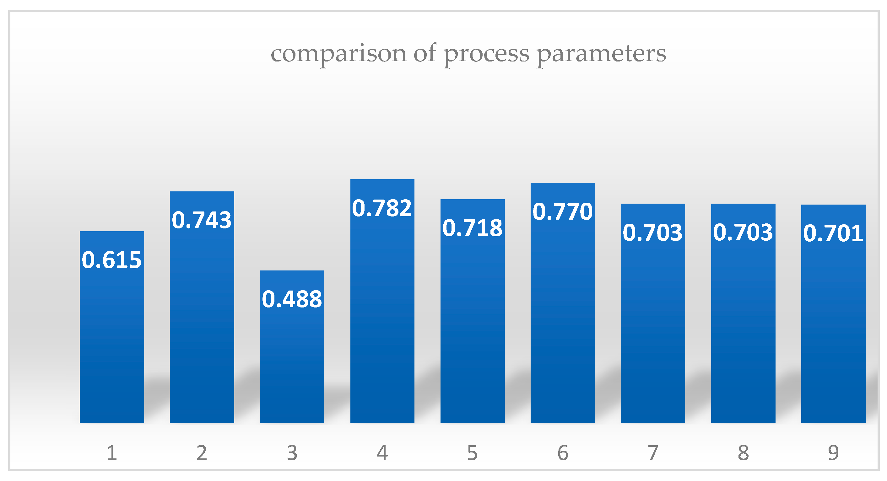
The resulting relational quality scores, according to dependence (30), are shown in Figure 3. The higher the integral relational score, the better the experimental outcome and the closer it is to the ideal normalized value.

As can be seen from the calculated values presented in Figure 3, the fourth sample has the highest value for the multiple quality indicator ($\gamma =0.782$). The values of the technological mode parameters used to obtain this sample correspond most closely to this indicator. Consequently, the quality indicators and technological parameters corresponding to this mode can be used as target parameters (indicated in Formulas (13)–(17) by the subscript index ‘0’) to calculate the margin of safety (MS).

4.3. Calculation of Regression Coefficients in Dependencies for Margins of Safety

The defined target process parameters (

Table 7. Target process characteristics.

№	Parameters	Type	Value
1	Layer thickness, t mm	Min	0.05
2	Layer thickness, t mm	Max	0.06
3	Scanning step, h mm	Min	0.065
4	Scanning step, h mm	Max	0.09
5	Power, P W	Min	229
6	Power, P W	Max	257
7	Scanning speed, v mm	Min	750
8	Scanning speed, v mm	Max	800
9	$\mathrm{Tensile}\mathrm{strength},{\sigma }_{\min }$ MPa	Min	740
10	$\mathrm{Yield}\mathrm{strength},{\sigma }_{02\min }$ MPa	Min	464
11	$\mathrm{Relative}\mathrm{elongation},{\delta }_{\min }$, %	Min	55
12	$\mathrm{Roughness},{Rz}_{max}$, µm	Max	21
13	$\mathrm{Scanning}\mathrm{step},h_0$ mm	Target parameter	0.09
14	$\mathrm{Scanning}\mathrm{speed},v_0$ mm/s	Target parameter	750
15	$\mathrm{Layer}\mathrm{thickness},t_0$ mm	Target parameter	0.06
16	$\mathrm{Power},P_0$ W	Target parameter	229

), based on the test results (Table 4), enable us to determine the unknown coefficients in the margin of safety dependencies (13)–(17) by solving the linear equation system (21). As a result, the following dependencies are obtained:

$$\begin{array}{l}M{S}_{V\min }\le \left({\displaystyle \frac{v}{750}}\right)\left({\displaystyle \frac{h}{0.090}}\right)\left({\displaystyle \frac{t}{0.06}}\right)\\ M{S}_{\sigma \min }\le 1.00541{\left({\displaystyle \frac{P/v}{0.3047}}\right)}^{0.803186}{\left({\displaystyle \frac{h}{0.09}}\right)}^{-0.143683}{\left({\displaystyle \frac{t}{0.06}}\right)}^{-0.361245}\\ M{S}_{\delta \min }\le 1.00873{\left({\displaystyle \frac{P/v}{0.3047}}\right)}^{2.37696}{\left({\displaystyle \frac{h}{0.09}}\right)}^{-0.33188}{\left({\displaystyle \frac{t}{0.06}}\right)}^{-1.23246}\\ M{S}_{Rz\max }\le 1.00649{\left({\displaystyle \frac{P/v}{0.3047}}\right)}^{-0.507737}{\left({\displaystyle \frac{h}{0.09}}\right)}^{0.099496}{\left({\displaystyle \frac{t}{0.06}}\right)}^{0.343456}\end{array},$$

(34)

The proportion of the variance of the dependent variable explained by the regression model under consideration is determined by the coefficient of determination (35).

$$\begin{array}{l}M{S}_{\sigma \min }{:\mathrm{R}}^2=0.819\\ M{S}_{\delta \min }:{\mathrm{R}}^2=0.838\\ M{S}_{R\max }:{\mathrm{R}}^2=0.760\end{array}$$

(35)

4.4. Optimization of Process Parameters

Taking into account the obtained values of the coefficients of influence of technological factors, the matrix A in (22) takes the following form:

$$A=\left[\begin{array}{ccccc}0& 1& 1& 1& 0\\ 0.803186& -0.803186& -0.143683& -0.361245& 0.005391\\ 2.37696& -2.37696& -0.33188& -1.23246& 0.00869\\ -0.507737& 0.507737& 0.099496& 0.343456& 0.006465\\ 0& 0& 0& 0& 1\end{array}\right],$$

(36)

The following vector of significance coefficients from dependence (23) was set to solve the optimization problem:

$$C=\left[\begin{array}{ccccc}10& 1& 1& 1& 0\end{array}\right],$$

(37)

The value of the coefficient $c_V=10$ in Equation (37) indicates the importance of productivity in the target function (23). Linear programming optimization was carried out using the simplex method. The vector X of the optimal variable values from dependencies (22) was obtained as a result of the optimization process.

$$X=X_{opt}=\left[\begin{array}{ccccc}0.1154& 0.0645& 0& 0& 1\end{array}\right],$$

(38)

For the given values of the vector X, the target function assumes a value:

Table 8. Constraint values at the optimal X values.

${\mathit{A}}_{\mathit{e}\mathit{n}}$					${\mathit{A}}_{\mathit{e}\mathit{n}}\cdot \mathit{X}$	Sign	${\mathit{B}}_{\mathit{e}\mathit{n}}$
0	1	1	1	0	0.0645	$\ge$	0
0.8032	−0.8032	−0.1437	−0.3612	0.0054	0.0463	$\ge$	0.00539
2.3770	−2.3770	−0.3319	−1.2325	0.0087	0.1297	$\ge$	0.00869
−0.5077	0.5077	0.0995	0.3435	0.0065	−0.0194	$\le$	0.00646
1	0	0	0	0	0.1154	$\ge$	0
−1	0	0	0	0	−0.1154	$\ge$	−0.11540
0	1	0	0	0	0.0645	$\ge$	0.00000
0	−1	0	0	0	−0.0645	$\ge$	−0.06450
0	0	1	0	0	0.0000	$\ge$	−0.32540
0	0	−1	0	0	0.0000	$\ge$	0

shows all the constraint values in matrix form (25), based on the optimal variable values (39).

$$R{F}_{\sum }=C\cdot A\cdot X=0.80157,$$

(39)

Table 9. Optimized L-DED characteristics.

No	Process Parameter	Type	Value
1	Scanning step, mm	Optimized	0.09
2	Scanning speed, mm/s	Optimized	800
3	Layer thickness, mm	Optimized	0.06
4	Power, W	Optimized	257
5	$\mathrm{Margins}\mathrm{of}\mathrm{safety}\mathrm{for}\mathrm{tensile}\mathrm{strength},M{S}_{\sigma }^1$	Estimated	1.0474
6	$\mathrm{Margins}\mathrm{of}\mathrm{safety}\mathrm{for}\mathrm{relative}\mathrm{elongation},M{S}_{\delta }^1$	Estimated	1.1385
7	$\mathrm{Margins}\mathrm{of}\mathrm{safety}\mathrm{for}\mathrm{Rz},M{S}_R^1$	Estimated	0.9808
8	$\mathrm{Margins}\mathrm{of}\mathrm{safety}\mathrm{for}\mathrm{performance},M{S}_V^1$	Estimated	1.067

shows the computed natural response results for the optimized values of the vector of variables X, as defined in dependence (38). As can be seen from the analysis of Table 8 (row 4) and Table 9 (row 7), increasing the layer thickness from 0.05 to 0.06 mm resulted in the surface roughness requirements not being met, which is understandable from the viewpoint of process physics. However, reducing the surface roughness requirements will improve other quality characteristics, compensating for the loss in this one.

4.5. Experimental Verification of the Adequacy of the Optimization Results

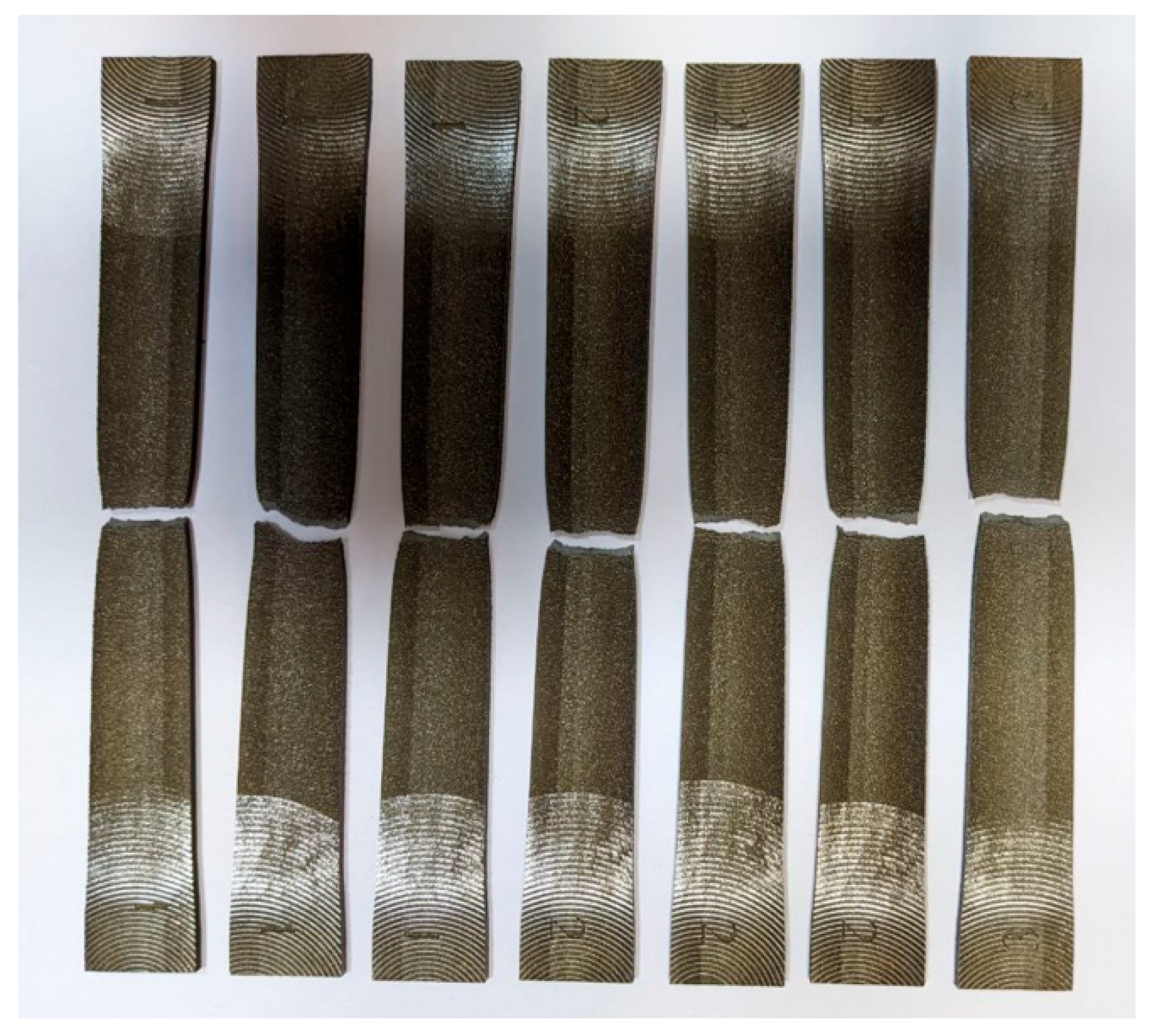
To verify the adequacy of the process parameter optimization results (Table 9) for L-PBF, verification experiments were carried out on the same flat specimens without heads, with dimensions of 140 × 20 × 30 mm, according to DIN EN ISO 6892:1998, using the process parameters given in

Table 10. Design of verification experiments.

№	Technological Mode	Power, W	Scanning Speed, mm/s	Scanning Step, mm	Layer Thickness, mm	Linear Energy Density, W/mm
1	Target (T)	229	750	0.090	0.06	0.305
2	Optimal (O)	257	800	0.090	0.06	0.321
3	Control (C)	229	800	0.090	0.06	0.286

(3–4 specimens each). The process parameters of technological mode (O) correspond to the calculated optimum parameters. The grown specimens were then subjected to tensile tests (Figure 4).

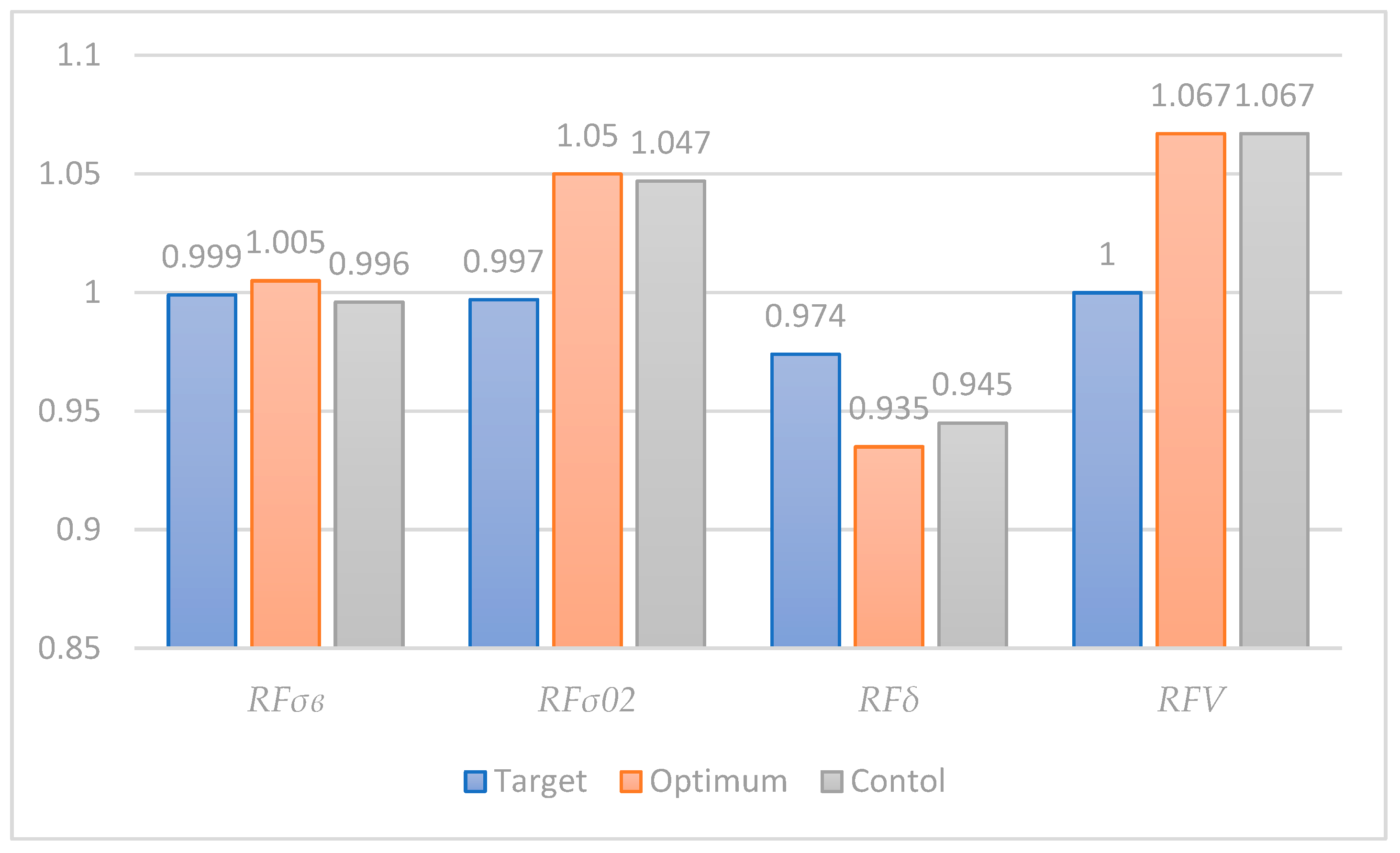
The test results are presented in

Table 11. Results of verification experiments.

Specimen N-M	${\mathit{\sigma }}_{\mathbf{B}}$, MPa		$\frac{\mathit{m}\mathit{e}\mathit{a}\mathit{n}{\mathit{\sigma }}_{\mathbf{B;}}}{\mathit{st}.\mathit{deviation}}$	${\mathit{\sigma }}_{02}$ MPa	$\frac{\mathit{m}\mathit{e}\mathit{a}\mathit{n}{\mathit{\sigma }}_{02}}{\mathit{st}.\mathit{deviation}}$	δ, %	$\frac{\mathit{m}\mathit{e}\mathit{a}\mathit{n}\mathit{\delta }}{\mathit{st}.\mathit{deviation}}$
1-1	(T)	744	${\displaystyle \frac{739.5}{5.26}}$	465	${\displaystyle \frac{462.5}{10.34}}$	52.66	${\displaystyle \frac{53.55}{1.302}}$
1-2		734		456		52.91
1-3		736		453		53.15
1-4		744		476		55.48
2-1	(O)	744	${\displaystyle \frac{743.3}{0.577}}$	487	${\displaystyle \frac{487.0}{1.00}}$	51.06	${\displaystyle \frac{51.4}{0.626}}$
2-2		743		488		52.14
2-3		743		486		51.05
3	(C)	737	737	486	486	51.95	51.95

and Figure 5. The test specimens were assigned numbers N–M, where N represents the technological mode from Table 10 and M represents the specimen’s order number.

5. Discussion

The optimization technique described above has been tested. It is designed around the proposed multi-criteria optimization parameters, which are the logarithms of the safety margins from quality characteristics. It reduces process variability by redefining process parameters within a limited search area. This approach is similar to Taguchi’s approach, which is based on estimating quality losses according to mean square deviation and the deviation of product characteristics from the target value.

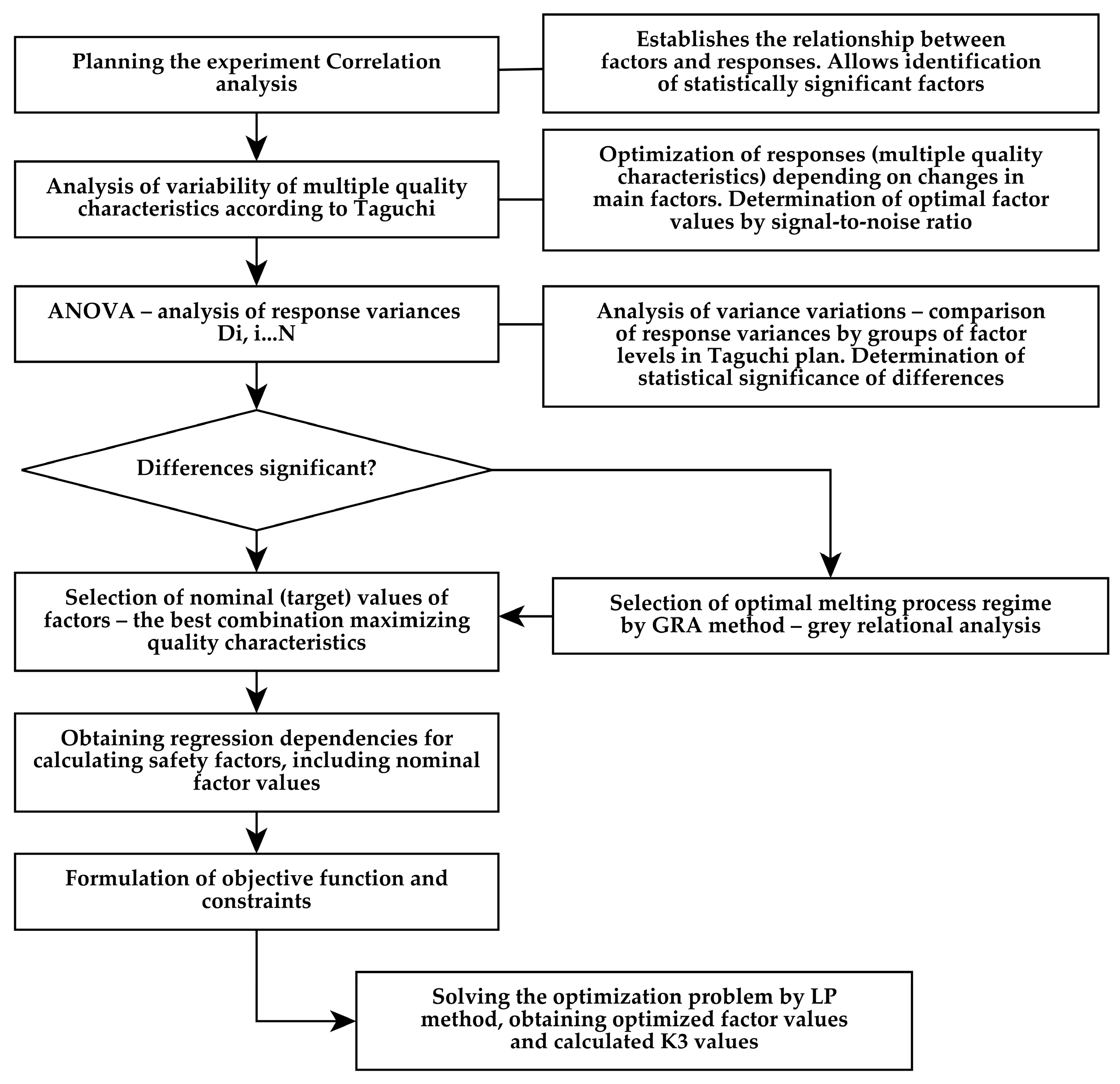
The solution scheme of the aforementioned optimization problem is presented in Figure 6.

This study uses orthogonal Taguchi DoE and the Taguchi method itself in the first stage. The main objective of this stage is to determine the target process parameters, which will be used for further optimization. According to Taguchi principles, only the influence of the independent factors (i.e., the process parameters) is considered; the pairwise interactions of the factors and the higher-order interactions are not taken into account. If the process variability is high, as an analysis of variance (ANOVA) of the results of the first stage shows, it is statistically unreliable to consider the responses of the process to be a result of the independent factors. In this case, the optimal values of the process parameters, obtained by maximizing the S/N ratio, are not statistically reliable.

Instead, the process mode is selected from the experimental plan whose responses correspond to the target function as closely as possible. The Grey relational analysis (GRA) method can be used for this purpose.

Analysis of the results of verification experiments according to the data in Table 11 shows that the parameters of the optimized alloying process provide samples with mechanical properties that are not inferior to those obtained using the target process parameters (T), with a tensile strength that exceeds the latter by 5% and a conditional yield strength that exceeds the latter by 5%.

Despite the fact that the ductility of the samples was 4% lower than the ductility of the samples fused at the nominal mode, a 6.7% increase in process productivity was achieved by increasing layer thickness. This fact allows us to state that the optimization objective was achieved.

The key result achieved as a result of the optimization is a significant reduction in process variability. Thus, the RMS for tensile strength decreased by nine times, for conditional yield strength by ten times, for relative elongation by two times. The reduction in RMS as a parameter was not included directly in the target function of the optimization process. At the same time, the reward functions, which are defined as logarithms of the shifted margins of safety, are additively included in the target function. If there is an increase in process variability, i.e., a decrease in MS relative to the response for the target process parameters, then the corresponding RF reward function and the target function decrease sharply near zero with negative values of the logarithm in RF.

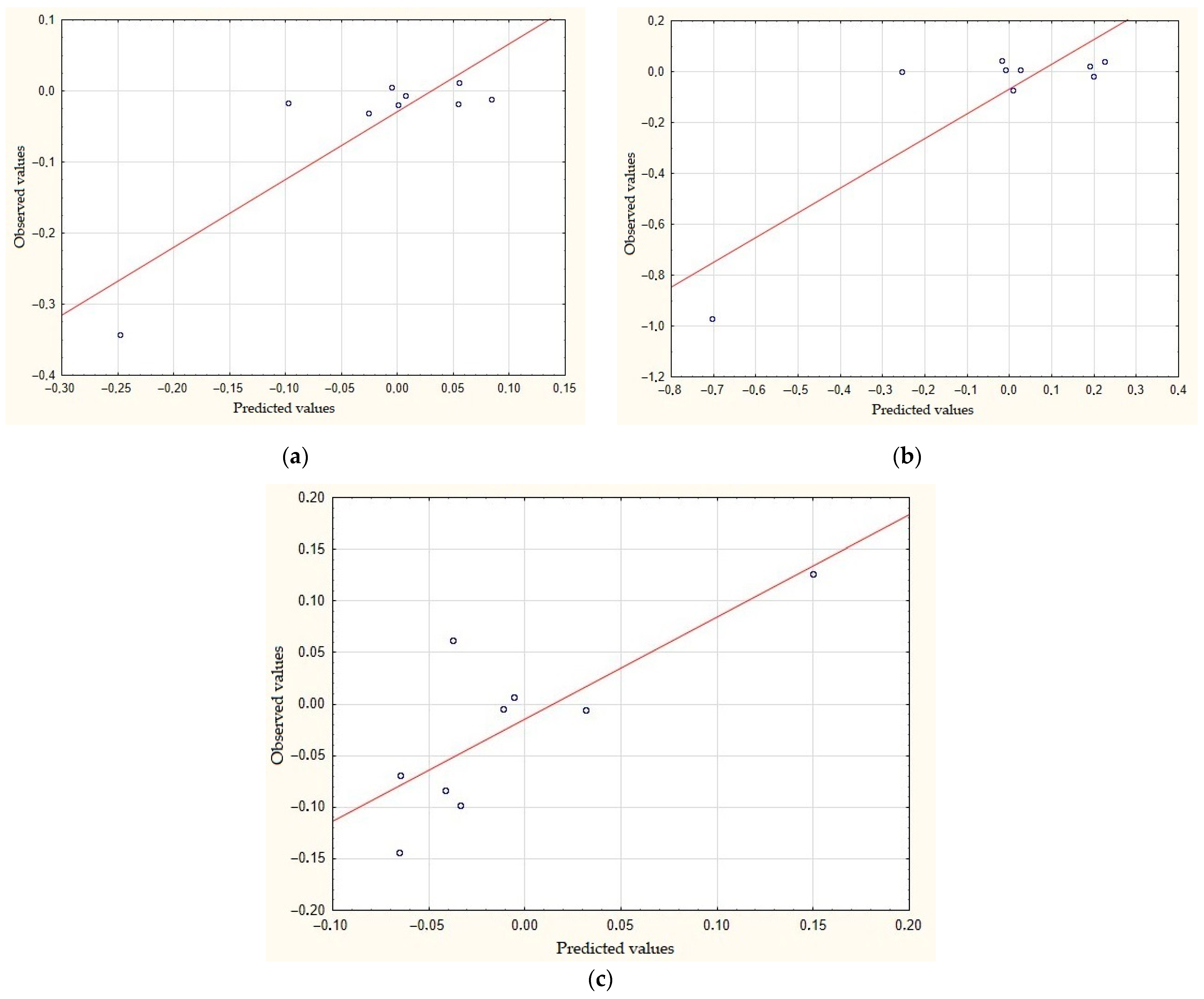
This can clearly be seen if we consider the RF dependence plots (21), for which the constants were found from nonequalities (34) in the form of a comparison between the predicted and observed values of dependence (see Figure 7).

Indeed, according to Taguchi’s calculations of the signal-to-noise (S/N) ratio, the area of technological parameters within the following boundaries corresponds to the area of stable S/N ratio values: power (W) [229–257], laser beam speed (mm/s) [750–800], and scanning step (mm) [0.065–0.09]. The optimized values of the technological parameters fall inside this stable range.

6. Conclusions

• A new metric for optimizing technological regimes is proposed—the reward function (RF), which considers process variability. The RF is the opposite of the quality loss function (QLF) proposed by Taguchi, which depends on the mean square deviation (MSD) and the difference between the product characteristic and the target value. However, unlike the signal-to-noise ratio (S/N), which is Taguchi’s measure of variability, the RF is treated as the logarithm of the margin of safety of the quality characteristic. The safety factor is equal to the ratio of the obtained quality characteristic value to the target (design) value. When the reserve coefficient is less than 1, the RF becomes sharply negative. The additivity peculiar to logarithms enables us to set the target function for optimizing technological modes as a sum of reward functions for quality characteristics, where each summand is multiplied by a significance coefficient for the respective characteristic beforehand. This approach enables the optimization problem to be formulated in terms of linear programming.
• It should be noted that the proposed approach is only effective within the vicinity of the optimal technological parameters. The boundaries of this region are robust due to the multifactorial nature and variability of the external conditions of the L-PBF process. Ranking the priorities of quality characteristics and introducing constraints using the proposed technology makes it possible to obtain the required optimal combination of characteristics within this area. Further research will analyse the robustness of constraints using the penalty function method.
• The specified approach was tested in the optimization of the technological processes for the L-PBF of AISI 321 Cr-Ni-high alloy steel powder. The resulting optimized alloying process regimes increased productivity by 6.7%. The mechanical properties of the resulting alloy are equal to those of the samples alloyed using the previously recommended regime in terms of ultimate strength and exceed the latter by 5% in terms of conditional yield strength. A significant reduction in process variability was achieved. Thus, the RMS decreased by nine times for tensile strength, by ten times for conditional yield strength, and by two times for relative elongation.

References

1. Mazur, M.; Selvakannan, P.R. Laser Powder Bed Fusion—Principles, Challenges, and Opportunities. In Additive Manufacturing for Chemical Sciences and Engineering; Springer Nature: Singapore, 2022; pp. 77–108. [Google Scholar]
2. Wang, D.; Yang, Y.; Liu, Y.; Bai, Y.; Tan, C. Factors Affecting the Manufacturing Quality of Laser Powder Bed Fusion. In Laser Powder Bed Fusion of Additive Manufacturing Technology; Additive Manufacturing Technology; Springer: Singapore, 2024; pp. 35–58. [Google Scholar]
3. Gatto, A.; Gatto, M.L.; Groppo, R.; Munteanu, D.; Mengucci, P. Influence of laser powder bed fusion process parameters on the properties of CuZn42 components: Case study of the laser surface energy density. Prog. Addit. Manuf. 2023, 8, 843–855. [Google Scholar] [CrossRef]
4. Buhairi, M.A.; Foudzi, F.M.; Jamhari, F.I.; Sulong, A.B.; Radzuan, N.A.M.; Muhamad, N.; Mohamed, I.F.; Azman, A.H.; Harun, W.S.W.; Al-Furjan, M.S.H. Review on volumetric energy density: Influence on morphology and mechanical properties of Ti6Al4V manufactured via laser powder bed fusion. Prog. Addit. Manuf. 2023, 8, 265–283. [Google Scholar] [CrossRef]
5. Kan, W.H.; Chiu, L.N.S.; Lim, C.V.S.; Zhu, Y.; Tian, Y.; Jiang, D.; Huang, A. A critical review on the effects of process-induced porosity on the mechanical properties of alloys fabricated by laser powder bed fusion. J. Mater. Sci. 2022, 57, 9818–9865. [Google Scholar] [CrossRef]
6. Templeton, W.F.; Hinnebusch, S.; Strayer, S.T.; To, A.C.; Pistorius, P.C.; Narra, S.P. A mechanistic explanation of shrinkage porosity in laser powder bed fusion additive manufacturing. Acta Mater. 2024, 266, 119632. [Google Scholar] [CrossRef]
7. Cao, S.; Zo-u, Y.; Lim, C.V.S.; Wu, X. Review of laser powder bed fusion (LPBF) fabricated Ti6Al-4V: Process, post-process treatment, microstructure, and property. Light Adv. Manuf. 2021, 2, 20. [Google Scholar] [CrossRef]
8. Kan, W.H.; Gao, M.; Zhang, X.; Liang, E.; Chiu, N.S.L.; Lim, C.V.S.; Huang, A. The influence of porosity on Ti-6Al-4V parts fabricated by laser powder bed fusion in the pursuit of process efficiency. Int. J. Adv. Manuf. Technol. 2022, 119, 5417–5438. [Google Scholar] [CrossRef]
9. Koutiri, I.; Pessard, E.; Peyre, P.; Amlou, O.; De Terris, T. Influence of SLM process parameters on the surface finish, porosity rate and fatigue behavior of as-built Inconel 625 parts. J. Mater. Process. Technol. 2018, 255, 536–546. [Google Scholar] [CrossRef]
10. Ahmed, N.; Barsoum, I.; Haidemenopoulos, G.; Al-Rub, R.K.A. Process parameter selection and optimization of laser powder bed fusion for 316L stainless steel: A review. J. Manuf. Process. 2022, 75, 415–434. [Google Scholar] [CrossRef]
11. Giorgetti, A.; Baldi, N.; Palladino, M.; Ceccanti, F.; Arcidiacono, G.; Citti, P. A Method to Optimize Parameters Development in L-PBF Based on Single and Multitracks Analysis: A Case Study on Inconel 718 Alloy. Metals 2023, 13, 306. [Google Scholar] [CrossRef]
12. Wen, S.; Wang, C.; Zhou, Y.; Duan, L.; Wei, Q.; Yang, S.; Shi, Y. High-density tungsten fabricated by selective laser melting: Densification, microstructure, mechanical and thermal performance. Opt. Laser Technol. 2019, 116, 128–138. [Google Scholar] [CrossRef]
13. Giri, N.C.; Das, M.N. Design and Analysis of Experiments; Wiley: New Delhi, India, 1986. [Google Scholar]
14. Khaimovich, A.I.; Stepanenko, I.S.; Smelov, V.G. Optimization of Selective Laser Melting by Evaluation Method of Multiple Quality Characteristics. IOP Conf. Ser. Mater. Sci. Eng. 2018, 302, 012067. [Google Scholar] [CrossRef]
15. Fanya, A.; Haruman, E.; Mohd Shahriman, A. Optimization of Multi-Objective Taguchi Method for Hybrid Thermochemical Treatment Applied to AISI 316LVM Biological Grade Stainless Steel. In Reference Module in Materials Science and Materials Engineering; Elsevier: Amsterdam, The Netherlands, 2019. [Google Scholar] [CrossRef]
16. Nath, R.; Murugesan, K. Optimization of Double Diffusive Mixed Convection in a Bfs Channel Filled with Alumina Nanoparticle Using Taguchi Method and Utility. Concept. Sci. Rep. 2019, 9, 19536. [Google Scholar] [CrossRef]
17. Liu, Y.; Liu, C.; Liu, W.; Ma, Y.; Tang, S.; Liang, C.; Cai, Q.; Zhang, C. Optimization of Parameters in Laser Powder Deposition AlSi10Mg Alloy Using Taguchi Method. Opt. Laser Technol. 2019, 111, 470–480. [Google Scholar] [CrossRef]
18. Manjunath, B.; Vinod, A.; Abhinav, K.; Verma, S.; Sankar, M.R. Optimisation of Process Parameters for Deposition of Colmonoy Using Directed Energy Deposition Process. Mater. Today Proc. 2020, 26, 1108–1112. [Google Scholar] [CrossRef]
19. Dong, G.; Marleau-Finley, J.; Zhao, Y.F. Investigation of Electrochemical Post-Processing Procedure for Ti-6AL-4V Lattice Structure Manufactured by Direct Metal Laser Sintering (DMLS). Int. J. Adv. Manuf. Technol. 2019, 104, 3401–3417. [Google Scholar] [CrossRef]
20. Liu, Y.; Wu, Z.; Wang, Q.; Zhao, L.; Zhang, X.; Gao, W.; Xu, J.; Song, Y.; Song, X.; Zhang, X. Optimization of Parameters in Laser Powder Bed Fusion TA15 Titanium Alloy Using Taguchi Method. Crystals 2022, 12, 1385. [Google Scholar] [CrossRef]
21. Yang, B.; Lai, Y.; Yue, X.; Wang, D.; Zhao, Y. Parametric Optimization of Laser Additive Manufacturing of Inconel 625 Using Taguchi Method and Grey Relational Analysis. Scanning 2020, 2020, 9176509. [Google Scholar] [CrossRef]
22. Jiang, H.-Z.; Li, Z.-Y.; Feng, T.; Wu, P.-Y.; Chen, Q.-S.; Feng, Y.-L.; Li, S.-W.; Gao, H.; Xu, H.-J. Factor Analysis of Selective Laser Melting Process Parameters with Normalised Quantities and Taguchi Method. Opt. Laser Technol. 2019, 119, 105592. [Google Scholar] [CrossRef]
23. Carley, K.M.; Kamneva, N.Y.; Reminga, J. Response Surface Methodology; Center for Computational Analysis of Social and Organizational Systems: Pittsburgh, PA, USA, 2004; p. 32. [Google Scholar]
24. Dada, M.; Popoola, P.; Mathe, N.; Pityana, S.; Adeosun, S. Parametric Optimization of Laser Deposited High Entropy Alloys Using Response Surface Methodology (RSM). Int. J. Adv. Manuf. Technol. 2020, 109, 2719–2732. [Google Scholar] [CrossRef]
25. Pant, P.; Chatterjee, D.; Nandi, T.; Samanta, S.K.; Lohar, A.K.; Changdar, A. Statistical Modelling and Optimization of Clad Characteristics in Laser Metal Deposition of Austenitic Stainless Steel. J. Braz. Soc. Mech. Sci. Eng. 2019, 41, 283. [Google Scholar] [CrossRef]
26. ElSayed, M.A.; Ghazy, M.; Youssef, Y.; Essa, K. Optimization of SLM Process Parameters for Ti6Al4V Medical Implants. Prototyp. J. 2019, 25, 433–447. [Google Scholar] [CrossRef]
27. Marmarelis, M.G.; Ghanem, R.G. Data-Driven Stochastic Optimization on Manifolds for Additive Manufacturing. Comput. Mater. Sci. 2020, 181, 109750. [Google Scholar] [CrossRef]
28. Dongari, S.; Davidson, M.J. Multi response optimization of Inconel 625 wire arc deposition for development of additive manufactured components using Grey relational analysis (GRA). Metallurg. Mater. Eng. 2021, 27, 177–192. [Google Scholar] [CrossRef]
29. Bhadrakali, A.; Narayana, K.; Prabhu, T.; Reddy, Y. Optimization of mechanical properties of ER-4043 specimens fabricated by WAAM process through Grey Relational Analysis. IOP Conf. Ser. Mater. Sci. Eng. 2021, 1055, 012047. [Google Scholar] [CrossRef]
30. Khaimovich, A.; Erisov, Y.; Smelov, V.; Agapovichev, A.; Petrov, I.; Razhivin, V.; Bobrovskij, I.; Kokareva, V.; Kuzin, A. Interface quality indices of Al–10Si–Mg aluminum alloy and Cr18–Ni10–Ti stainless-steel bimetal fabricated via selective laser melting. Metals 2021, 11, 172. [Google Scholar] [CrossRef]
31. Agapovichev, A.V.; Khaimovich, A.I.; Smelov, V.G.; Kokareva, V.V.; Alekseev, V.P.; Zemlyakov, E.V.; Kovchik, A.Y. Optimization of L-PBF Process Parameters for Defect Reduction and Mechanical Strength of Ni-Cr-Mo-Nb Superalloy Using Multi-Objective Methods. Materials 2025, 18, 1743. [Google Scholar] [CrossRef] [PubMed]
32. Khaimovich, A.; Balyakin, A.; Oleynik, M.; Meshkov, A.; Smelov, V. Optimization of Process Parameters for Powder Bed Fusion Additive Manufacturing Using a Linear Programming Method: A Conceptual Framework. Metals 2022, 12, 1976. [Google Scholar] [CrossRef]
33. Taguchi, G.; Wu, Y. Introduction to Off-Line Quality Control; Central Japan Quality Control Association: Tokyo, Japan, 1985. [Google Scholar]
34. Kackar, R.N. Off-Line Quality Control, Parameter Design, and the Taguchi Method. In Quality Control, Robust Design, and the Taguchi Method; Dehnad, K., Ed.; Springer: Boston, MA, USA, 1989. [Google Scholar] [CrossRef]
35. Burr, A.; Cheatham, J. Mechanical Design and Analysis, 2nd ed.; Prentice-Hall: Englewood Cliffs, NJ, USA, 1995; Section 5.2. [Google Scholar]
36. Juvinall, R. Stress, Strain, and Strength; McGraw-Hill: Columbus, OH, USA, 1967; Section 14.13; p. 295. [Google Scholar]
37. NASA. Structural Design and Test Factors for Spaceflight Hardware; NASA-STD-5001; NASA: Washington, DC, USA, 2008; Section 3.
38. AIAA. Space Systems—Structures, Structural Components, and Structural Assemblies; AIAA S-110; AIAA: Reston, VA, USA, 2005; Section 4.2. [Google Scholar]
39. DIN EN ISO 6892-1:1998; Metallic Materials—Tensile Testing—Part 1: Method of Test at Room Temperature. ISO: Geneva, Switzerland, 1998.
40. ISO 21920-2:2021; Surface Texture—Part 2: Terms, Definitions and Surface Texture Parameters. ISO: Geneva, Switzerland, 2021.
Figure 1. (A) AISI 321 particle size distribution and (B) roughness measurement directions.
Metals 15 01027 g001
Figure 2. Expected signal-to-noise ratio (S/N).
Metals 15 01027 g002
Figure 3. Relational estimates of sample quality by coefficient γ i (33).
Metals 15 01027 g003
Figure 4. Flat specimens after tensile testing in the verification experiment.
Metals 15 01027 g004
Figure 5. The margins of safety for the target, optimum and control specimens.
Metals 15 01027 g005
Figure 6. Technique for solving the optimization problem.
Metals 15 01027 g006
Figure 7. Observed vs predicted values of regard functions according to dependence (31): (a) tensile strength, (b) relative elongation, and (c) roughness (Rz).
Metals 15 01027 g007