Article

A Meshless Multiscale and Multiphysics Slice Model for Continuous Casting of Steel

1
Faculty of Mechanical Engineering, University of Ljubljana, Aškerčeva 6, SI-1000 Ljubljana, Slovenia
2
Institute of Metals and Technology, Lepi pot 11, SI-1000 Ljubljana, Slovenia
3
Štore Steel d.o.o., Železarska cesta 3, SI-3220 Štore, Slovenia
*
Author to whom correspondence should be addressed.
Metals 2025, 15(9), 1007; https://doi.org/10.3390/met15091007
Submission received: 28 April 2025 / Revised: 13 June 2025 / Accepted: 23 June 2025 / Published: 10 September 2025

Abstract

A simple Lagrangian travelling slice model has been successfully used to predict the relations between the process parameters and the strand temperatures in the continuous casting of steel. The present paper aims to include a simple macrosegregation, grain structure and mechanical stress and deformation model on top of the thermal slice framework. The basis of all the mentioned models is the slice heat-conduction model that considers the complex heat extraction mechanisms in the mould, with the sprays, rolls, and through radiation. Its main advantage is the fast calculation time, which is suitable for the online control of the caster. The macroscopic thermal and species transfer models are based on the continuum mixture theory. The macrosegregation model is based on the lever rule microsegregation model. The thermal conductivity and species diffusivity of the liquid phase are artificially enhanced to consider the convection of the melt. The grain structure model is based on cellular automata and phase-field concepts. The calculated thermal field is used to estimate the thermal contraction of the solid shell, which, in combination with the metallostatic pressure, drives the elastic-viscoplastic solid-mechanics models. The solution procedure of all the models is based on the meshless radial basis function generated finite difference method on the macroscopic scale and the meshless point automata concept on the grain structure scale. Simulation results point out the areas susceptible to hot tearing.

1. Introduction

Numerical simulations of the physical phenomena which occur during the continuous casting (CC) process [1,2,3,4,5,6,7,8,9] are crucial for setting up proper process parameters and dynamically regulating the process. In the framework of the slice model, heat transfer is split into the advection and conduction parts. In the casting direction, we consider only advection, while only conduction is considered in the plane perpendicular to the casting direction [10,11,12,13]. A slice model coupled with realistic material properties is a powerful tool for determining relations between the process parameters and the temperature field. Therefore, such a model determines the caster’s optimal casting parameters and estimates the possible design changes. The optimal casting parameters are associated with the maximum productivity of the caster, considering the limitations posed by the maximum allowed metallurgical length, minimum allowed solidified shell thickness at the mould exit, maximum allowed stresses, etc. These parameters depend on the format and steel grade. The model can also be used to estimate the design changes of the caster, such as improved spray cooling, positioning of the final electromagnetic stirrer, etc. Due to their high computational efficiency, online slice models are also essential for automating the caster.
The purpose of the present paper is to show how the thermal slice model can be upgraded to qualitatively predict columnar to equiaxed transition (CET) positions, composition inhomogeneities, and strand stresses and strains. We achieve this by coupling the thermal model with the grain structure, macrosegregation, and mechanical models as shown in Figure 1. The model can also estimate the need for more comprehensive multiphysics simulations that can be performed on high-performance systems only.
We apply the meshless radial basis function generated finite difference (RBF-FD) method [14,15,16,17] to solve the partial differential equations (PDEs) in the travelling slice. The RBF-FD method is also known in the literature as the local radial basis function collocation method (LRBFCM) [18,19]. As the finite difference method, the RBF-FD method approximates a spatial operator in a computational node as a sum of weighted field values from a local sub-domain. Researchers have successfully employed the RBF-FD method to model scientific and engineering problems, e.g., modelling turbulent fluid flow in the continuous casting of steel [20], elasto-plasticity [21], dendritic solidification [22,23,24,25,26], fluid flow and heat transfer [27,28], magnetohydrostatics [29], etc. We apply the point automata (PA) method [30] to simulate the grain structure evolution, i.e., the nucleation and growth of grains in the whole cross-section of a billet. The PA method is a meshless version of the cellular automata (CA) method [31,32,33,34,35,36]. While the CA method relies on regularly distributed cells, PA applies to randomly distributed points. Additionally, we simulate the growth of representative equiaxed grains using the phase-field (PF) method [37,38,39,40,41] to obtain an accurate description of the evolution of the solid-liquid interface morphology.
The described model of CC represents a first step in meshless modelling of casting, heat treatment [42], rolling [43,44], crack propagation [45], and cooling on a cooling bed [21] of the entire steel production path. The most important foreseen upgrades of the model will consider an improved mechanical model that will also consider strains in the casting direction and coupling of the microstructure model with CALPHAD database for coping with multi-component steel.

2. Materials and Methods

2.1. Thermal Model

The slice model considers the heat conduction in the plane perpendicular to the casting direction
( ρ h ) t = ( k T ) ,
where ρ , h , k , and T stand for density, enthalpy, thermal conductivity, and temperature. The following equations are shown for a binary system. However, a materials database is used to determine temperature-dependent material properties when simulating the casting of multi-component steels. The mixture enthalpy is given as [46]
h = f s h s + ( 1 f s ) h l ,
where f s is the solid fraction, and the subscripts s and l represent the solid and liquid phases, respectively. In the case of constant specific heat in each phase, the enthalpies in the solid and the liquid phase are determined as
h s = h r e f + c p s ( T T r e f ) ,   h l = h r e f + c p s ( T s o l T r e f ) + c p l ( T T s o l ) + h m ,
where h r e f , T r e f , c p , T s o l , and h m stand for reference enthalpy, reference temperature, specific heat, solidus temperature, and latent heat of melting. The mixture conductivity is given as
  k = f s k s + ( 1 f s ) k l .
We employ the lever rule as a supplementary micro-segregation relation
C = f s C s + ( 1 f s ) C l ,   C s = k p C l ,
where C and k p stand for concentration and partition coefficient. The temperature as a function of the concentration in the liquid phase is given as
T = T m + m l C l ,
where T m and m l stand for the solvent’s melting temperature and the liquidus line’s slope.

2.2. Mechanical Model

We employ the mechanical model in a small-deformation approximation. The strain is decomposed into elastic, thermal, and viscoplastic parts [11]. The thermal part is given as
ε t = I T r e f T α ( T ) d   T ,
where α ( T ) is the temperature-dependent coefficient of thermal expansion and I the identity tensor. We use the Garafalo law [47] to describe the viscoplastic part
ε ˙ v p = A 0 exp ( q / T ) σ e σ 0 n ,
where σ e stands for the equivalent Von Mises stress; the parameters A 0 , q , n , and σ 0 are determined from the least square fit of the high-temperature flow-stress data obtained from suitable steel material properties software or measurements. We account for the metallostatic pressure by introducing a body force f b = p m f s , where p m is the metallostatic pressure at the slice’s centre. In the equilibrium, the displacement field is determined by solving the following partial differential equation
p m f s = G 2 u + ( G + λ ) u + λ u + G u + u T     G ε v p ( 3 λ + 2 G ) ε t ,
where G and λ are the Lamé parameters. We employ the traction-free boundary conditions and neglect the mechanical contact with the mould and rolls. The impact of rolls on the mechanical state of the strand comes from two mechanisms. Firstly, there is a direct mechanical support from the rolls. The rolls need to support the full weight of the strand, and the stiffness of the strand allows the weight to be transferred from the unsupported sections to the roll contact positions. Since the 2D simplification prevents any load transfer along the casting direction, this mechanism cannot be reasonably accurately described in the model, so we neglect this mechanism. Secondly, the rolls contribute indirectly by intensively removing heat from the strand and in doing so, they introduce high thermal strain gradients near the roll contact area. This, in turn, triggers thermal stresses that are included in the mechanical model. Even the thermal effect on its own is enough to demonstrate some bulging between the rollers.

2.3. Grain Structure Model

We simulate the heterogeneous nucleation and dendrite growth in the grain structure model. We employ the log-normal distribution to describe the distribution of the nucleation density n over the undercooling Δ T
d n d Δ T = n max 2 π Δ T σ exp 1 2 log Δ T log Δ T μ Δ T σ 2 ,
where n m a x , Δ T σ , and Δ T μ are maximum nucleation density, scale, and mean of the undercooling. We employ the LGK [48,49] model to obtain the dendrite tip growth velocity as a function of undercooling Δ T
v = D l 5.51 π 2 ( m l ( 1 k p ) C 0 ) 1.5 Γ s l Δ T 2.5 ,
where D l , C 0 , and Γ s l stand for solute diffusivity in the liquid phase, initial concentration, and Gibbs-Thomson coefficient.

2.4. Phase-Field Model

The PF model consists of two PDEs, one for the PF ϕ and one for the dimensionless supersaturation U . Values ϕ = 1 and ϕ = 1 represent solid and liquid phases, respectively. The PF model from [50] is rewritten in the framework of frozen temperature approximation [51] where the dimensionless temperature θ is considered an input parameter. As in similar studies [52,53,54], the PF model with negligible attachment kinetics is applied. θ and U are defined concerning the reference point in the phase diagram, with the equilibrium temperature T e and the equilibrium concentration in the liquid phase C l e as
U = C l C l e ( 1 k p ) C l e , θ = T T e m l ( 1 k p ) C l e .
The governing equation for PF reads as
( 1 + ( 1 k 0 ) U ) a 2 ( n ) ϕ t = ϕ ϕ 3 1 ϕ 2 2 λ θ + U + a 2 ( n ) ϕ + ξ = x , y ξ | ϕ | 2 a ( n ) a ( n ) ( ξ ϕ ) ,
where a and λ stand for the anisotropy function and the coupling parameter, respectively. Cubic symmetry of the interfacial energy is accounted for with the selection
a ( n ) = 1 3 ϵ 4 + 4 ϵ 4 ( n x 4 + n y 4 ) ,
where the normal n is defined as n = ( n x , n y ) = ϕ / | ϕ | and ϵ 4 represents the strength of the anisotropy. The governing equation for U is given as
1 2 1 + k p ( 1 k p ) ϕ U t = 1 2 1 + ( 1 k p ) U ϕ t + D ¯ ( ϕ ) U + a a t ( 1 + ( 1 k p ) U ) ϕ t n ,
where D ¯ and a a t stand for the dimensionless diffusivity and the antitrapping current coefficient, respectively. They are defined as
D ( ϕ ) = k p D s + D l + ( k p D s D l ) ϕ / 2 , a a t = 1 2 2 1 k p D s D l ,
where D s and D l stand for the diffusivities of solute in the solid and the liquid phase, respectively. The relation between dimensional D and dimensionless D ¯ is given as D ¯ = D τ 0 / W 0 2 , where W 0 and τ 0 stand for the interface thickness and characteristic time of attachment, respectively. The time and spatial coordinates in the PDEs are dimensionless. They are measured in units of W 0 and τ 0
W 0 = d 0 1 α 1 λ , τ 0 = d 0 2 D l α 2 α 1 2 λ 3
where d 0 stands for the chemical capillary length; α 1 = 0.8839 and α 2 = 0.6267 are the PF constants [55]. Chemical capillary length is defined as
d 0 = Γ s l m l ( 1 k p ) C l e .
Interface thickness W 0 is the only free parameter of the PF model. The PF model correctly captures the underlying solidification problem when W 0 is much smaller than the characteristic diffusivity length of the solidification problem. The thermal noise is introduced in the simulations by reformulating the PDE for PF as [53]
ϕ ( t 0 + Δ t ) = ϕ ( t 0 ) + Δ t ϕ t t 0 + ξ β i ( 1 ϕ 2 ) Δ t / 2 ,
where ξ controls the magnitude of the noise and β i is a random number generated from a flat distribution in the range [−0.5, 0.5] in each computational point. The value ξ = 0.01 is used in this study.

2.5. Macrosegregation Model

The macrosegregation model accounts for the solute diffusion in the liquid phase
( ρ C ) t = ( ρ f l D l C l ) .
Solving Equations (1) and (20) require the determination of T , C l , and f s at given C and h . They are set by solving a system of nonlinear equations given by Equations (2), (3), (5) and (6). We artificially increase the liquid diffusivity of the solute by a factor of 10 to mimic the influence of the turbulent flow [10]. The factor is a free parameter that must be set appropriately to match the experimental results. Too small values cannot predict the correct macrosegregation profiles, e.g., centerline segregation. Too large values predict too large centerline segregation. The factor may also be determined by comparing it with the results of the fluid flow models.

3. Numerical Methods

3.1. RBF-FD Method

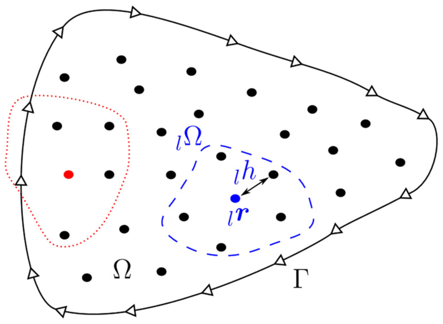
The RBF-FD method [14,15] is based on the local interpolation of the field values. For clarity, the method is presented for the case of scalar fields; however, the same procedure is used for higher-ranked fields. For each l r Ω , l = 1 , , N , where N is the number of computational nodes in Ω , a local sub-domain Ω l , centred at l r is generated. Ω l consists of l r and its N l 1 nearest nodes, as schematically shown in Figure 2. The RBF-FD method is based on interpolating the field value over a local sub-domain using radial basis functions (RBFs). A RBF centred at l r is denoted as Φ l ( r ) . The interpolation problem is augmented with m monomials ψ i l ( r ) .
A scalar field η at r Ω Γ , where is l r the computational node closest to r , is approximated as
η ( r ) i = 1 N l α i l Φ i l ( r ) + i = 1 m α l N l + i ψ i ( r ) = i = 1 N l + m α i l Ψ i l ( r ) ,
where α i l is an interpolation coefficient and Ψ i l is either a RBF or a monomial. Application of Equation (21) for each node in a local sub-domain yields a system of linear equations. The linear boundary condition B r with right-hand value b ( r ) applies to Equation (21) if r Γ . The interpolation problem can be written in a matrix form as
i = 1 N l + m A j i l α i l = l γ j ,
where
A j i l = Ψ i l ( l r j ) if   l r j Ω B ( l r j ) Ψ i ( l r j ) if   l r j Γ ψ j ( l r i ) if   j > l N   and   i l N 0 otherwise ,
where
γ j l = η ( l r j ) if   l r j Ω b ( l r j ) if   l r j Γ 0 otherwise .
The approximation from Equation (21) is used to evaluate any linear differential operator D applied to a scalar field η ( r ) in r Ω , while the boundary condition is analytically satisfied. Applying D to Equation (21) yields
D η ( r ) i = 1 N l + m α i l D Ψ i ( r ) .
By calculation inverse of the matrix, defined by Equation (15), Equation (17), applied at lr , is rewritten as
D η ( l r ) k = 1 N l + m γ k l i = 1 N l + m A i k 1 l D Ψ i ( l r ) .
Equation (18) can now be written in a standard finite-difference-structure
D η ( l r ) k = 1 N l γ k l w k l ,
where w k l are finite-difference-like coefficients, defined as
w k l = i = 1 N l + m A i k 1 l D Ψ i ( l r ) .

3.2. Solution of the Thermal and Macrosegregation Models

We solve the thermal and macrosegregation models using the regular node distribution with the spacing h t h e r m a l = 1   mm . We employ the forward Euler scheme for the temporal discretisation with the time step
Δ t = 0.2 h t h e r m a l 2 max ( D T s , D T l , D l ) ,   D T = k ρ c p ,
where D T is the thermal diffusivity. For the spatial discretisation, we employ the RBF-FD method with five nodes in a local sub-domain, multiquadrics as RBFs, and first-order augmentation with monomials. The shape parameter of muliquadrics is determined for each local sub-domain independently according to the interpolation matrix’s targeted condition number of 10 20 .

3.3. Solution of the Grain Structure Model

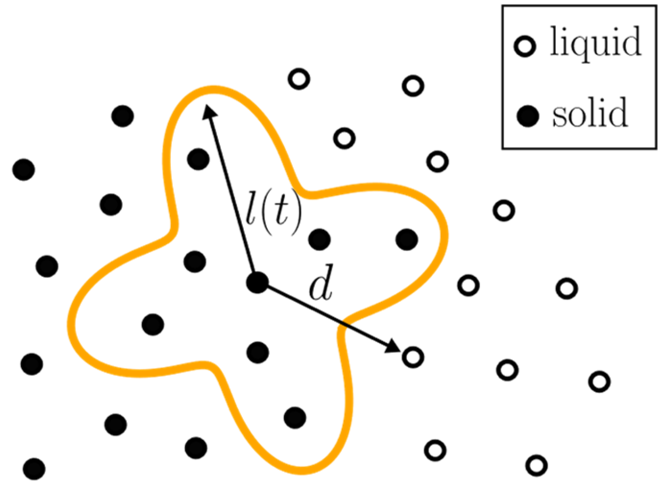
We employ the PA method [30] to simulate heterogeneous nucleation and dendrite growth. First, we randomly distribute the points in the computational domain. For each point, we determine the neighbourhood, which consists of the points within the circle with a radius R P A = 1.5 h P A , where h P A stands for the characteristic spacing between the two neighbouring points, set to h P A = 0.1   mm in the current study. We define a state for each point, either solid or liquid. Additionally, we assign a grain number and orientation angle θ to each point in the solid state. The algorithm checks points every Δ t P A = Δ t / M , where M is the number of divisions of Δ t . A liquid point changes its state to solid if
r < V P A Δ T Δ T + δ ( Δ T ) d n d ( Δ T ) d ( Δ T ) ,
where r is a random number in the range ( 0 , 1 ] , V P A is the volume represented by a point, and δ ( Δ T ) stands for the change of Δ T during one time step. A random grain number and a random orientation angle θ are assigned to the newly nucleated point. After nucleation, a point starts capturing its liquid neighbours. The size of a primary dendrite arm is calculated as
l ( t ) = t 0 t v ( Δ T ) d t ,
where t 0 is the time at which the nucleation occurred. The liquid point is captured by the solid neighbour if
d l ( t ) 1 + α 2 1 α 2 cos 4 ( θ ϕ ) ,
where d is the distance between the solid and liquid points, α stands for the dendrite envelope ratio, and ϕ is given as
ϕ = arctan ( d y / d x ) ,
where d = d x 2 + d y 2 . If a solid point captures a liquid neighbour, the captured liquid point changes its state to solid; the capturer’s grain number and orientation angle are assigned to the captured liquid point. Figure 3 shows the PA dendrite growth algorithm.

3.4. Solution of the PF Model

We employ the forward Euler scheme for time stepping and the RBF-FD method for the discretisation of spatial linear differential operators. The dimensionless time step is calculated as
Δ t = 0.3 1 4 h P F 2 max ( D ¯ l , 1 / ( 1 ϵ 4 ) )
where h P F stands for dimensionless spacing beween neighbouring nodes. In the RBF-FD method, we apply thirteen nodes in a local sub-domain, fifth-degree polyharmonic splines as RBFs, and second-order augmentation with monomials. It is suggested to use at least twice the number of augmentation monomials for the number of nodes in a local support domains. Additionally, symmetric stencils result in better stability; hence, we set the number of nodes in a local support domain to thirteen, since the number of monomials in the second-order augmentation is equal to six. The calculations are accelerated by a quadtree-based space-time adaptive algorithm [23]. The minimum dimensionless node spacing is set to h P F = 0.4 .

3.5. Solution of the Mechanical Model

We employ the implicit Euler scheme for temporal discretisation of the mechanical model. For the spatial discretisation, we employ the RBF-FD method with eighteen nodes in a local sub-domain, polyharmonic splines as RBFs, and second-order augmentation with monomials. The thermal and thermomechanical models are one-way coupled; the temperature field from the thermal model drives the solution of the thermomechanical model. We employ the adaptive time stepping; the time step depends on the nonlinear solver’s convergence rate. The node distribution is adaptive, too, with the highest density of computational nodes in the mushy zone as shown in Figure 4. We ensure spacing of 0.5 mm in the mushy zone, 1 mm in the solid phase, and 5 mm in the liquid phase.

4. Test Problem Definition and Numerical Results

4.1. Thermal and Macrosegregation Model

The capabilities of the multiscale and multiphysics slice model are demonstrated by solving a test case proposed in [10]. The computational domain is a square with an edge length equal to 140 mm. The square slice travels in the casting direction with the constant casting speed v c a s t = 1.75   m / min . The position of the slice is determined as
z ( t ) = z 0 + v c a s t ( t t 0 ) ,
where z 0 and t 0 are the initial slice coordinate and the initial time, respectively; they are set to zero in the present study. In the slice model, the time integration is equivalent to the moving of the slice in the casting direction according to Equation (26). The boundary condition for the thermal model considers cooling in the mould ( z < 0.8   m ) and the spray area ( z 0.8   m )
k T n = h m o l d ( T T c o o l ) ,   k T n = h s p r a y ( T T c o o l ) ,
where n is the outward-facing normal to the boundary of the computational domain, h m o l d and h s p r a y are the heat transfer coefficients in the mould and spray region, respectively, and T c o o l is the cooling temperature. The heat transfer coefficients and the cooling temperature are set to h m o l d = 2000   W / ( m 2 K ) , h s p r a y = 800   W / ( m 2 K ) , and T c o o l = 303   K . We apply the zero-flux Neumann boundary conditions when solving the macrosegregation model. We consider the casting of Fe-0.8wt.%C steel ( C 0 = 0.8 wt . % C ). The initial superheat of the melt is set to 20   K . Table 1 shows the material properties used in the study.
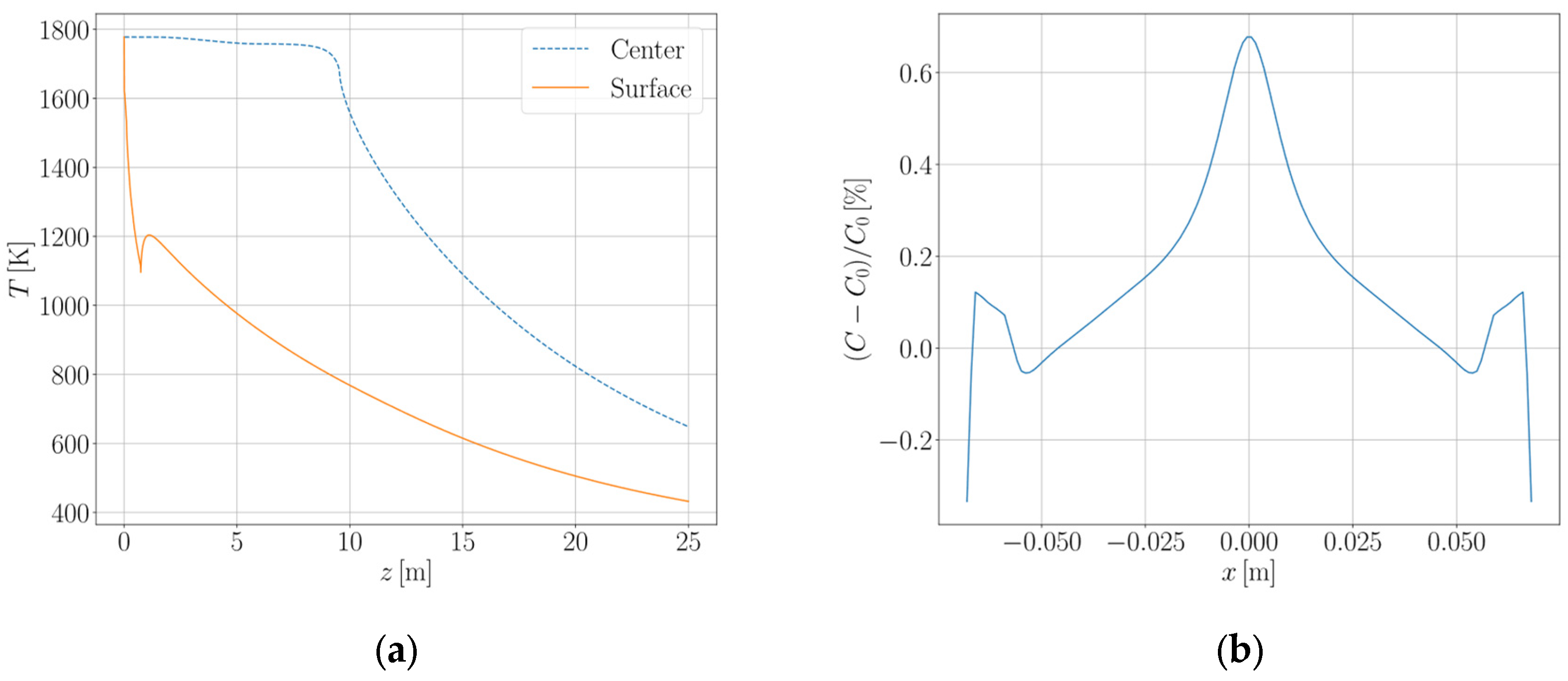
Figure 5a shows the temperature at the centre and the surface (west edge’s centre) of the slice. The temperature at the surface experiences a large drop due to fast cooling in the mould. After the slice moves out of the mould, the temperature rises, followed again by a more gradual decrease due to cooling in the spray area. At the centre, the temperature remains close to the initial temperature until the solidification front reaches the middle of the slice; at that point, we observe a significant decrease in the temperature. Figure 5b shows the final carbon concentration profile as a function of x in the middle of the slice ( y = 0   mm ). At the strand’s surface, we observe a large drop of the concentration which corresponds to the large temperature drop in the mould cooling area. Since zero-flux Neumann boundary conditions are applied, the carbon-depleted area at the surface yields small positive peaks of carbon concentration close to the surface. The turbulent flow is responsible for the negative peaks at | x | 5.5   cm and the large positive central segregation.

4.2. Results of the Grain Structure Model

In the PA model, we set the number of divisions of the time step from the thermal model to M = 100 . We apply two nucleation densities, one at the surface and one in the bulk of the strand. The following relations are applied to map general 3-D densities onto 2-D densities [32]
n m a x , s u r f 3 D = π 4 ( n m a x , s u r f 2 D ) 2 ,   n m a x , b u l k 3 D = π 6 ( n m a x , b u l k 2 D ) 3 / 2 .
Table 2 shows the parameters used in the PA model.
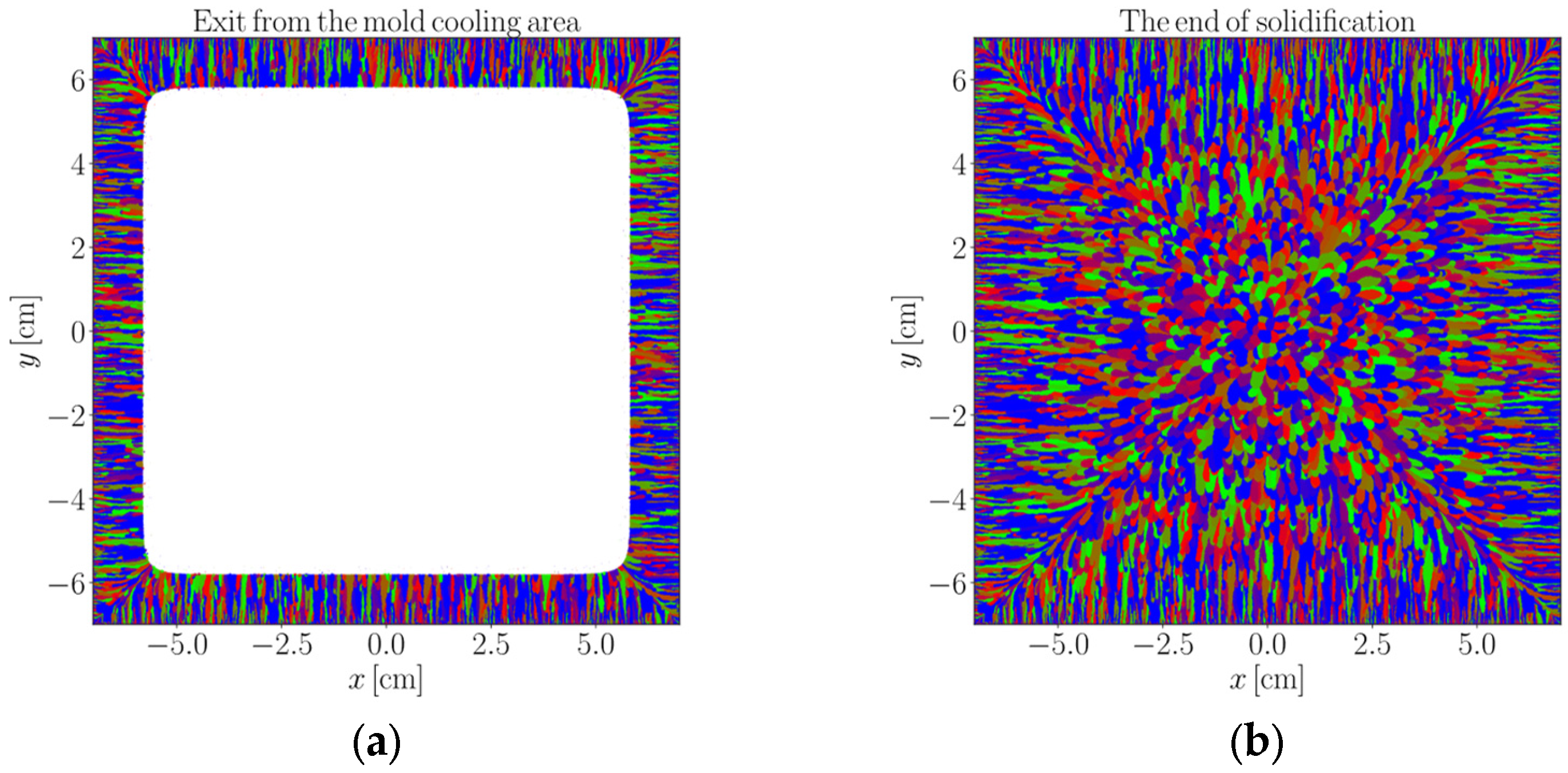
Figure 6 shows the grain structure at two slice positions. Many dendrite grains nucleate at the strand’s surface, resulting in a thin equiaxed region near the surface. The grains start to grow in a large temperature gradient, where the grains whose orientation is closer to the direction perpendicular to the strand’s surface overgrow the misoriented dendrite grains. This yields the development of the columnar zone. The temperature gradient decreases as we move from the strand’s surface. This increases the thickness of the undercooled liquid ahead of the columnar grains and, therefore, increases the probability of the nucleation of new grains. The newly nucleated grains block the columnar dendrites at a certain distance from the surface and yield a large central zone of equiaxed grains.

4.3. Results of the PF Model

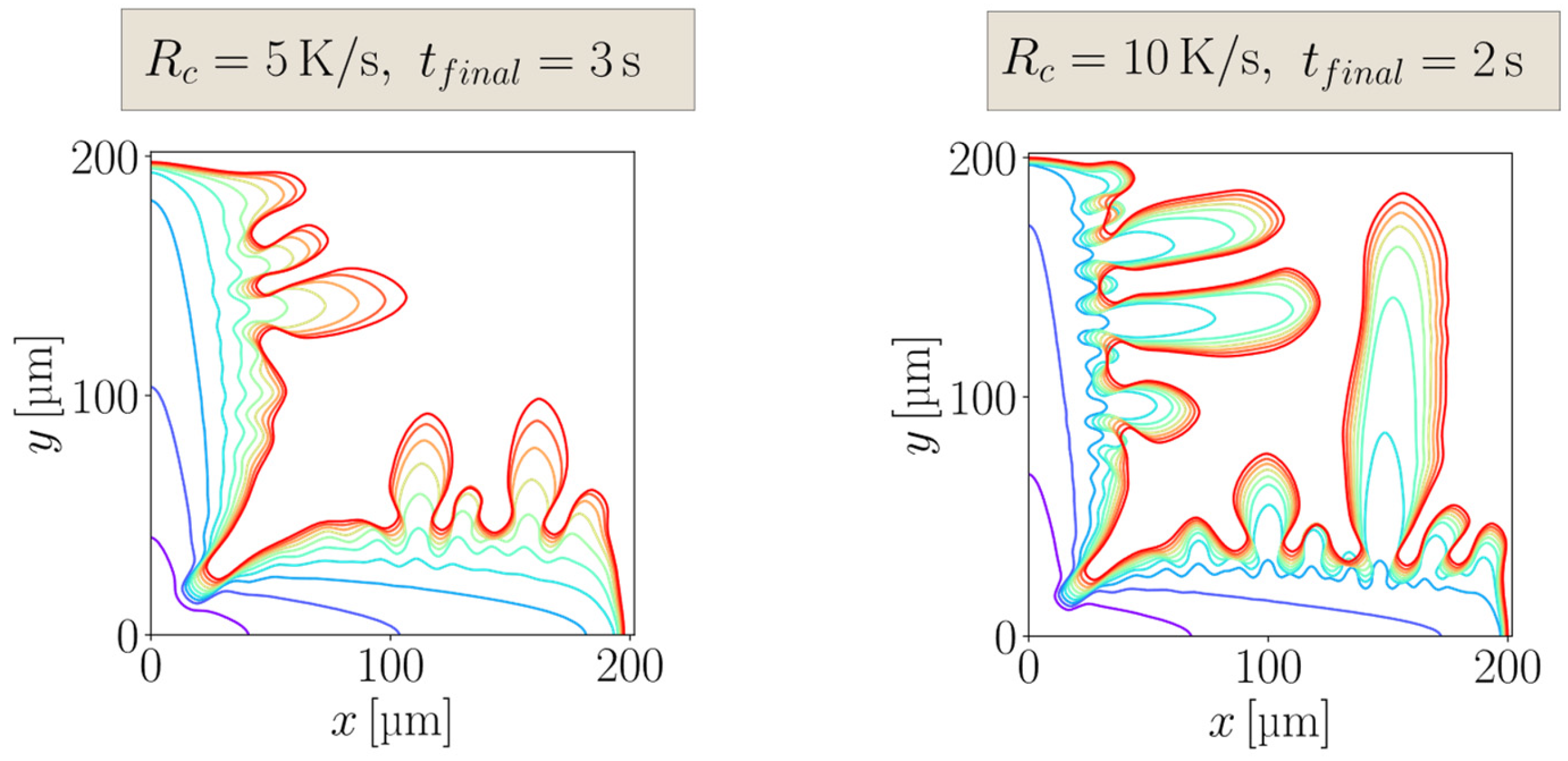
In the PF model, we simulate the growth of a representative equiaxed dendritic grain. The grains simulated by the PA model grow at different cooling rates, which dictate their final size. The nucleation and growth competition processes also hugely impact the grain’s size. We chose two representative cooling rates R c = 5   K / s and R c = 10   K / s and the size of the dendrite’s trunk L = 400   μ m . Due to cubic symmetry, we apply mirroring boundary conditions and simulate the growth of one quarter of a dendrite with ϵ 4 = 0.04 and W 0 = 50 d 0 ; the material properties from Table 1 are used. Figure 7 shows the evolution of the solid-liquid interface for both cooling rates. The dendrite starts to grow from an initial circular nucleus. The growth velocity increases with time due to the imposed cooling rate till a neighbouring dendrite, simulated by zero flux boundary conditions, suppresses the growth. After that, the primary trunk becomes coarser and coarser with time. The solid-liquid interface becomes perturbed over time due to the induced thermal noise. Different perturbations start to compete with each other, which yields the evolution of secondary branches while other perturbations are suppressed. The morphologies at two different cooling rates are quite similar in the initial unconstrained stage of growth. When a dendrite tip reaches the boundary and coarsening starts, the secondary branches develop faster for R c = 10   K / s due to the higher solidification driving force. Consequently, the primary trunk is less coarse and secondary branches are developed to a greater extent for R c = 10   K / s .

4.4. Results of the Mechanical Model

Table 3 shows the parameters of the mechanical model used in the present study; they correspond to high-strength steel.
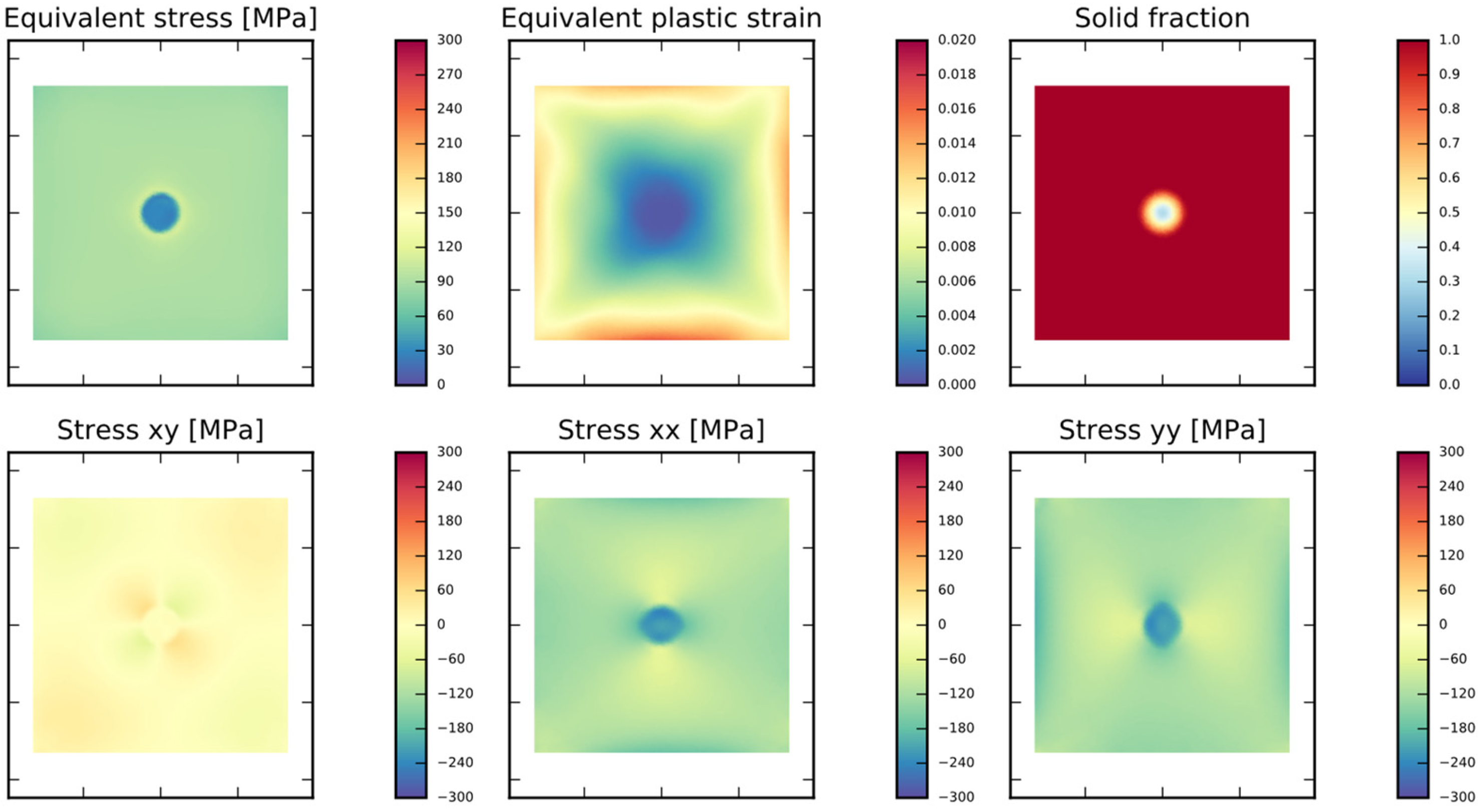
Figure 8 shows the equivalent stress, components of the stress tensor and solid fraction at the mould exit. Figure 9 shows the same near the end of the metallurgical length, where the entire billet has almost solidified. We can notice that the plastic deformations start accumulating in the billet’s corners. Still, in later stages, the plastic deformation mostly accumulates along the sides of the billet, which are in tension. From the plots of the stress tensor components, we also notice that, except for the corners, the material is in compression at the start of the casting process.

5. Conclusions

In the present paper, we have joined essential physical phenomena that a simple slice model can describe qualitatively. We have demonstrated the capabilities of the model based on a simple test case. The developed model has been verified by comparison with the surface temperature measurements and solid strand thickness, Bauman prints and dimensional measurements. A very good agreement with the industry measurements was found, especially for the surface temperature at different casting positions (range ± 10 K). It is productively used in the Štore-Steel company billet caster for all the possible purposes defined in the introduction. The model can be extended to reasonably account for external fields, such as electro-magnetic stirring, by modifying the liquid thermal conductivity as a function of the Lorentz force magnitude. It also forms a part of the comprehensive through-process modelling of the steel plant, based on the chain of physics-based and artificial intelligence models. This model represents a pioneering multiphysics approach in which all the partial differential equations are solved by the strong-form meshless RBF-FD method.

Author Contributions

Conceptualisation, B.Š.; software, B.M., T.D. and R.V.; validation, R.V.; writing—original draft preparation, B.Š.; writing—review and editing, B.M., T.D. and R.V.; supervision, B.Š.; project administration, B.Š.; funding acquisition, B.Š. All authors have read and agreed to the published version of the manuscript.

Funding

This work was supported by the Slovenian Research and Innovation Agency (ARIS) in the framework of programme group P2-0162, project L2-3173, co-financed by Štore-Steel company (www.store-steel.si) and a post-doctoral basic project Z2-4479.

Data Availability Statement

The original contributions presented in this study are included in the article. Further inquiries can be directed to the corresponding author.

Acknowledgments

The authors acknowledge the Štore-Steel company (www.store-steel.si) to agree on the publication of the present paper.

Conflicts of Interest

Author Robert Vertnik was employed by the company Štore Steel d.o.o. The remaining authors declare that the research was conducted in the absence of any commercial or financial relationships that could be construed as a potential conflict of interest. The authors declare that this study received funding from the company Štore Steel d.o.o. The funder had the following involvement with the study: author Robert Vertnik participated in the development of the software and validation.

References

  1. Irving, W.R. Continuous Casting of Steel; Institute of Materials: London, UK, 1993; ISBN 978-0-901716-53-8. [Google Scholar]
  2. Dong, Q.; Zhang, J.; Yin, Y.; Wang, B. Three-Dimensional Numerical Modeling of Macrosegregation in Continuously Cast Billets. Metals 2017, 7, 209. [Google Scholar] [CrossRef]
  3. Yang, J.; Ji, Z.; Liu, W.; Xie, Z. Digital-Twin-Based Coordinated Optimal Control for Steel Continuous Casting Process. Metals 2023, 13, 816. [Google Scholar] [CrossRef]
  4. Kim, H.-S.; Kim, J.-J.; Oh, K.-S. A Simplified Model for Semi-Continuous Casting of Steel. J. Mater. Eng Perform 2023, 32, 4064–4070. [Google Scholar] [CrossRef]
  5. Klimeš, L.; Štětina, J. A Rapid GPU-Based Heat Transfer and Solidification Model for Dynamic Computer Simulations of Continuous Steel Casting. J. Mater. Process. Technol. 2015, 226, 1–14. [Google Scholar] [CrossRef]
  6. Li, C.; Thomas, B.G. Thermomechanical Finite-Element Model of Shell Behavior in Continuous Casting of Steel. Met. Mater. Trans. B 2004, 35, 1151–1172. [Google Scholar] [CrossRef]
  7. Ren, B.; Zhu, L.; Wang, H.; Chen, D. Numerical Simulation of Fluid Flow and Solidification in Round Bloom Continuous Casting with Alternate Final Electromagnetic Stirring. Metals 2025, 15, 605. [Google Scholar] [CrossRef]
  8. Li, Z.; Lu, Y.; Wang, R.; Li, G.; Cui, H. Numerical Simulation of Effects of Mold Cavity and Submerged Entry Nozzle on Flow, Heat Transfer and Solidification in Funnel-Type Molds for Thin Slab Casting. Metals 2025, 15, 183. [Google Scholar] [CrossRef]
  9. Li, Y.; He, W.; Zhao, C.; Liu, J.; Yang, Z.; Zhao, Y.; Yang, J. Mathematical Modeling of Transient Submerged Entry Nozzle Clogging and Its Effect on Flow Field, Bubble Distribution and Interface Fluctuation in Slab Continuous Casting Mold. Metals 2024, 14, 742. [Google Scholar] [CrossRef]
  10. Vušanović, I.; Vertnik, R.; Šarler, B. A Simple Slice Model for Prediction of Macrosegregation in Continuously Cast Billets. IOP Conf. Ser. Mater. Sci. Eng. 2012, 27, 012056. [Google Scholar] [CrossRef]
  11. Mavrič, B.; Dobravec, T.; Vertnik, R.; Šarler, B. A Meshless Thermomechanical Travelling-Slice Model of Continuous Casting of Steel. IOP Conf. Ser. Mater. Sci. Eng. 2020, 861, 012018. [Google Scholar] [CrossRef]
  12. Šarler, B.; Vertnik, R.; Lorbiecka, A.Z.; Vušanović, I.; Senčič, B. A Multiscale Slice Model for Continuous Casting of Steel. IOP Conf. Ser. Mater. Sci. Eng. 2012, 33, 012021. [Google Scholar] [CrossRef]
  13. Bazzaro, G.; De Bona, F. Effectiveness of Travelling Slice Modeling in Representing the Continuous Casting Process of Large Product Sections. Metals 2023, 13, 1505. [Google Scholar] [CrossRef]
  14. Flyer, N.; Fornberg, B.; Bayona, V.; Barnett, G.A. On the Role of Polynomials in RBF-FD Approximations: I. Interpolation and Accuracy. J. Comput. Phys. 2016, 321, 21–38. [Google Scholar] [CrossRef]
  15. Bayona, V.; Flyer, N.; Fornberg, B.; Barnett, G.A. On the Role of Polynomials in RBF-FD Approximations: II. Numerical Solution of Elliptic PDEs. J. Comput. Phys. 2017, 332, 257–273. [Google Scholar] [CrossRef]
  16. Bayona, V.; Flyer, N.; Fornberg, B. On the Role of Polynomials in RBF-FD Approximations: III. Behavior near Domain Boundaries. J. Comput. Phys. 2019, 380, 378–399. [Google Scholar] [CrossRef]
  17. Kolar-Požun, A.; Jančič, M.; Rot, M.; Kosec, G. Some Observations Regarding the RBF-FD Approximation Accuracy Dependence on Stencil Size. J. Comput. Sci. 2024, 79, 102284. [Google Scholar] [CrossRef]
  18. Šarler, B.; Vertnik, R. Meshfree Explicit Local Radial Basis Function Collocation Method for Diffusion Problems. Comput. Math. Appl. 2006, 51, 1269–1282. [Google Scholar] [CrossRef]
  19. Ali, I.; Hanoglu, U.; Vertnik, R.; Šarler, B. Assessment of Local Radial Basis Function Collocation Method for Diffusion Problems Structured with Multiquadrics and Polyharmonic Splines. Math. Comput. Appl. 2024, 29, 23. [Google Scholar] [CrossRef]
  20. Vertnik, R.; Mramor, K.; Šarler, B. Solution of Three-Dimensional Temperature and Turbulent Velocity Field in Continuously Cast Steel Billets with Electromagnetic Stirring by a Meshless Method. Eng. Anal. Bound. Elem. 2019, 104, 347–363. [Google Scholar] [CrossRef]
  21. Vuga, G.; Mavrič, B.; Hanoglu, U.; Šarler, B. A Hybrid Radial Basis Function-Finite Difference Method for Modelling Two-Dimensional Thermo-Elasto-Plasticity, Part 2: Application to Cooling of Hot-Rolled Steel Bars on a Cooling Bed. Eng. Anal. Bound. Elem. 2024, 159, 331–341. [Google Scholar] [CrossRef]
  22. Dobravec, T.; Mavrič, B.; Šarler, B. Reduction of Discretisation-Induced Anisotropy in the Phase-Field Modelling of Dendritic Growth by Meshless Approach. Comput. Mater. Sci. 2020, 172, 109166. [Google Scholar] [CrossRef]
  23. Dobravec, T.; Mavrič, B.; Šarler, B. Acceleration of RBF-FD Meshless Phase-Field Modelling of Dendritic Solidification by Space-Time Adaptive Approach. Comput. Math. Appl. 2022, 126, 77–99. [Google Scholar] [CrossRef]
  24. Dobravec, T.; Mavrič, B.; Zahoor, R.; Šarler, B. A Coupled Domain–Boundary Type Meshless Method for Phase-Field Modelling of Dendritic Solidification with the Fluid Flow. Int. J. Numer. Methods Heat Fluid Flow 2023, 33, 2963–2981. [Google Scholar] [CrossRef]
  25. Dobravec, T.; Mavrič, B.; Šarler, B. A Study on Different Implementations of Neumann Boundary Conditions in the Meshless RBF-FD Method for the Phase-Field Modelling of Dendrite Growth. Eng. Anal. Bound. Elem. 2025, 173, 106154. [Google Scholar] [CrossRef]
  26. Jiang, P.; Zheng, H.; Xiong, J.; Rabczuk, T. The Localized Radial Basis Function Collocation Method for Dendritic Solidification, Solid Phase Sintering and Wetting Phenomenon Based on Phase Field. J. Comput. Phys. 2025, 520, 113515. [Google Scholar] [CrossRef]
  27. Zamolo, R.; Bacer, L.; Miotti, D.; Nobile, E.; Munerato, M. RBF-FD Meshless Simulation of 3D Fully Developed Flow and Heat Transfer in Triply Periodic Minimal Surfaces. Int. J. Heat Mass Transf. 2025, 242, 126798. [Google Scholar] [CrossRef]
  28. Bacer, L.; Zamolo, R.; Miotti, D.; Nobile, E. Adaptive RBF-FD Meshless Solution of 3D Fluid Flow and Heat Transfer Problems. Eng. Anal. Bound. Elem. 2025, 179, 106367. [Google Scholar] [CrossRef]
  29. Mathews, N.H.; Flyer, N.; Gibson, S.E. Solving 3D Magnetohydrostatics with RBF-FD: Applications to the Solar Corona. J. Comput. Phys. 2022, 462, 111214. [Google Scholar] [CrossRef]
  30. Lorbiecka, A.Z.; Šarler, B. Simulation of Dendritic Growth with Different Orientation by Using the Point Automata Method. CMC Comput. Mater. Contin. 2010, 18, 69–104. [Google Scholar] [CrossRef]
  31. Gandin, C.A.; Rappaz, M. A Coupled Finite Element-Cellular Automaton Model for the Prediction of Dendritic Grain Structures in Solidification Processes. Acta Metall. Mater. 1994, 42, 2233–2246. [Google Scholar] [CrossRef]
  32. Rappaz, M.; Gandin, C.A. Probabilistic Modelling of Microstructure Formation in Solidification Processes. Acta Metall. Mater. 1993, 41, 345–360. [Google Scholar] [CrossRef]
  33. Reuther, K.; Rettenmayr, M. Perspectives for Cellular Automata for the Simulation of Dendritic Solidification—A Review. Comput. Mater. Sci. 2014, 95, 213–220. [Google Scholar] [CrossRef]
  34. Asle Zaeem, M.; Yin, H.; Felicelli, S.D. Modeling Dendritic Solidification of Al–3%Cu Using Cellular Automaton and Phase-Field Methods. Appl. Math. Model. 2013, 37, 3495–3503. [Google Scholar] [CrossRef]
  35. Krane, M.J.M.; Johnson, D.R.; Raghavan, S. The Development of a Cellular Automaton-Finite Volume Model for Dendritic Growth. Appl. Math. Model. 2009, 33, 2234–2247. [Google Scholar] [CrossRef]
  36. Chen, R.; Xu, Q.; Liu, B. Cellular Automaton Simulation of Three-Dimensional Dendrite Growth in Al–7Si–Mg Ternary Aluminum Alloys. Comput. Mater. Sci. 2015, 105, 90–100. [Google Scholar] [CrossRef]
  37. Chen, L.-Q. Phase-Field Models for Microstructure Evolution. Annu. Rev. Mater. Res. 2002, 32, 113–140. [Google Scholar] [CrossRef]
  38. Boettinger, W.J.; Warren, J.A.; Beckermann, C.; Karma, A. Phase-Field Simulation of Solidification. Annu. Rev. Mater. Res. 2002, 32, 163–194. [Google Scholar] [CrossRef]
  39. Steinbach, I. Phase-Field Models in Materials Science. Model. Simul. Mat. Sci. Eng. 2009, 17, 073001. [Google Scholar] [CrossRef]
  40. Nestler, B.; Choudhury, A. Phase-Field Modeling of Multi-Component Systems. Curr. Opin. Solid State Mater. Sci. 2011, 15, 93–105. [Google Scholar] [CrossRef]
  41. Karma, A.; Tourret, D. Atomistic to Continuum Modeling of Solidification Microstructures. Curr. Opin. Solid State Mater. Sci. 2016, 20, 25–36. [Google Scholar] [CrossRef]
  42. Liu, Q.; Hanoglu, U.; Rek, Z.; Šarler, B. Simulation of Temperature Field in Steel Billets during Reheating in Pusher-Type Furnace by Meshless Method. Math. Comput. Appl. 2024, 29, 30. [Google Scholar] [CrossRef]
  43. Hanoglu, U.; Šarler, B. Multi-Pass Hot-Rolling Simulation Using a Meshless Method. Comput. Struct. 2018, 194, 1–14. [Google Scholar] [CrossRef]
  44. Hanoglu, U.; Šarler, B. Developments towards a Multiscale Meshless Rolling Simulation System. Materials 2021, 14, 4277. [Google Scholar] [CrossRef]
  45. Ali, I.; Vuga, G.; Mavrič, B.; Šarler, B. Meshless Solution of the Crack Propagation in Brittle Elastic Material under Shear, Compressible and Tensile Loading. Eng. Fract. Mech. 2025, 323, 111207. [Google Scholar] [CrossRef]
  46. Bennon, W.D.; Incropera, F.P. A Continuum Model for Momentum, Heat and Species Transport in Binary Solid-Liquid Phase Change Systems—I. Model Formulation. Int. J. Heat Mass Transf. 1987, 30, 2161–2170. [Google Scholar] [CrossRef]
  47. Koric, S.; Thomas, B.G. Thermo-Mechanical Models of Steel Solidification Based on Two Elastic Visco-Plastic Constitutive Laws. J. Mater. Process. Technol. 2008, 197, 408–418. [Google Scholar] [CrossRef]
  48. Lipton, J.; Glicksman, M.E.; Kurz, W. Equiaxed Dendrite Growth in Alloys at Small Supercooling. Met. Mat Trans. A 1987, 18, 341–345. [Google Scholar] [CrossRef]
  49. Lipton, J.; Glicksman, M.E.; Kurz, W. Dendritic Growth into Undercooled Alloy Metals. Mater. Sci. Eng. 1984, 65, 57–63. [Google Scholar] [CrossRef]
  50. Ohno, M. Quantitative Phase-Field Modeling of Nonisothermal Solidification in Dilute Multicomponent Alloys with Arbitrary Diffusivities. Phys. Rev. E 2012, 86, 051603. [Google Scholar] [CrossRef]
  51. Echebarria, B.; Folch, R.; Karma, A.; Plapp, M. Quantitative Phase-Field Model of Alloy Solidification. Phys. Rev. E 2004, 70, 061604. [Google Scholar] [CrossRef] [PubMed]
  52. Boukellal, A.K.; Debierre, J.-M.; Reinhart, G.; Nguyen-Thi, H. Scaling Laws Governing the Growth and Interaction of Equiaxed Al-Cu Dendrites: A Study Combining Experiments with Phase-Field Simulations. Materialia 2018, 1, 62–69. [Google Scholar] [CrossRef]
  53. Tourret, D.; Karma, A. Growth Competition of Columnar Dendritic Grains: A Phase-Field Study. Acta Mater. 2015, 82, 64–83. [Google Scholar] [CrossRef]
  54. Xie, Y.; Dong, H.; Dantzig, J. Growth of Secondary Dendrite Arms of Fe–C Alloy during Transient Directional Solidification by Phase-Field Method. ISIJ Int. 2014, 54, 430–436. [Google Scholar] [CrossRef]
  55. Karma, A.; Rappel, W.-J. Quantitative Phase-Field Modeling of Dendritic Growth in Two and Three Dimensions. Phys. Rev. E 1998, 57, 4323. [Google Scholar] [CrossRef]
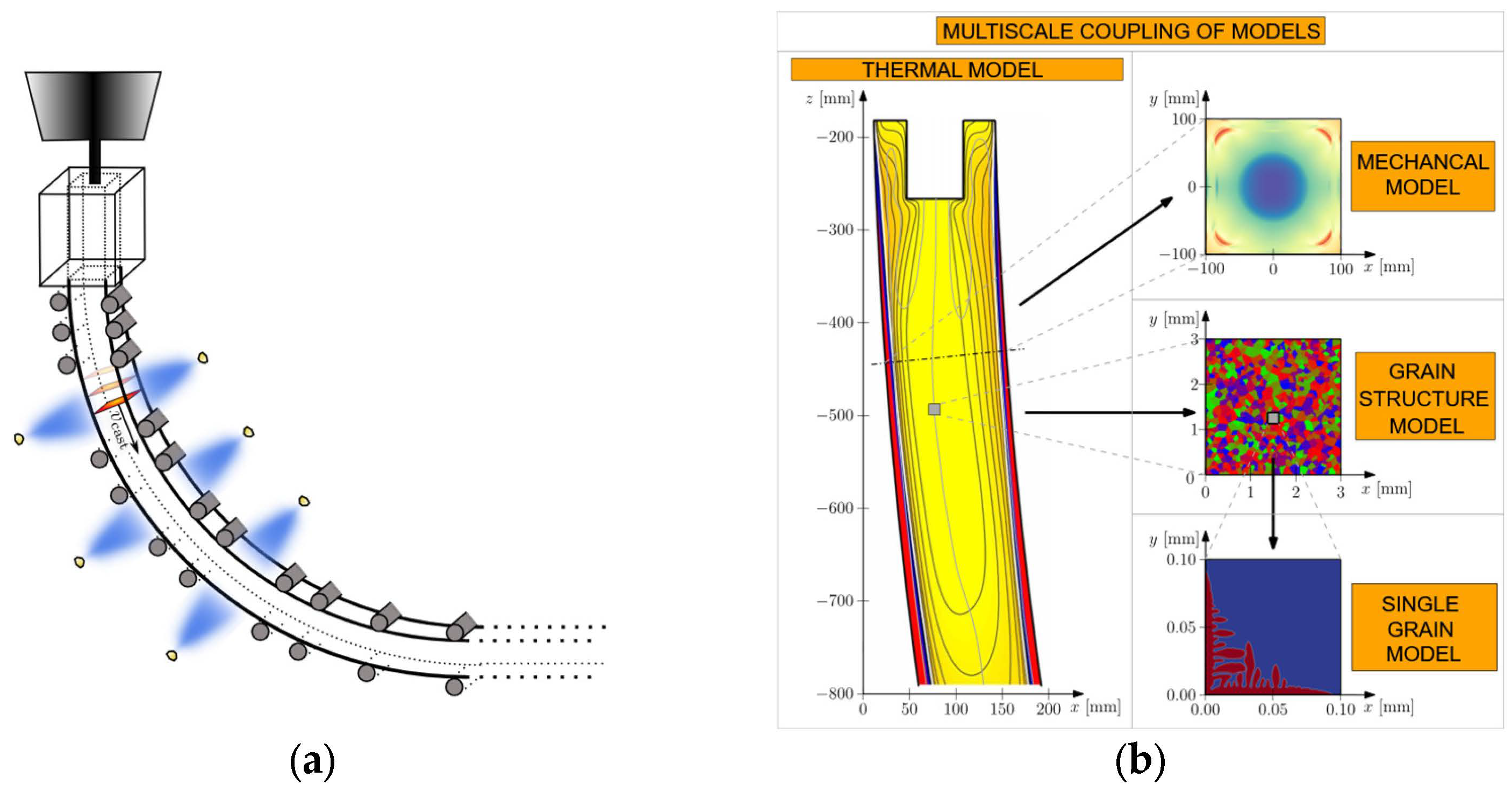
Figure 1. A scheme of (a) travelling slice model and (b) multiscale and multiphysics coupling for modelling continuous casting of steel.
Metals 15 01007 g001
Figure 2. A scheme of the interior (solid circles) and boundary (empty triangles) nodes lying in a computational domain Ω and boundary Γ . The dashed and dotted lines represent the boundaries of two local sub-domains.
Metals 15 01007 g002
Figure 3. A scheme of the algorithm for dendrite growth within the PA model.
Metals 15 01007 g003
Figure 4. Scheme of computational node distributions for four numerical models.
Metals 15 01007 g004
Figure 5. (a) Temperature at the centre and the surface (west edge’s centre) of the slice as a function of the casting coordinate. (b) Final carbon concentration profile in the middle of the slice.
Metals 15 01007 g005
Figure 6. Microstructure at two positions of the slice. (a) The exit of mould. (b) The end of solidification. Different colours represents different grain orientations.
Metals 15 01007 g006
Figure 7. Evolution of the solid-liquid interface for a single equiaxed grain at two cooling rates. Different colours represents different simulation times.
Metals 15 01007 g007
Figure 8. The results of the mechanical model at the exit from the mold cooling area.
Metals 15 01007 g008
Figure 9. The results of the mechanical model near the end of solidification.
Metals 15 01007 g009
Table 1. Physical and phase diagram properties of Fe-0.8wt.%C.
PropertySymbol[Unit]Value
Density ρ [ kg / m 3 ] 7870.0
Specific heat in liquid c p l [ J / ( kgK ) ] 1395.8
Specific heat in solid c p s [ J / ( kgK ) ] 824.9
Thermal conductivity in liquid k l [ W / ( mK ) ] 39.3
Thermal conductivity in solid k s [ W / ( mK ) ] 25.0
Latent heat of melting L m [ J / kg ] 2.71 × 10⁵
Solute diffusivity D l [ m 2 / s ] 1.36 × 10⁻⁹
Melting temperature of Fe T m [ K ] 1811.15
Eutectic temperature T e u t [ K ] 1427.15
Eutectic concentration C e u t [ wt . % C ] 4.3
Partition coefficient k p [ ] 0.521
Gibbs-Thomson coefficient Γ s l [ Km ] 3.0 × 10⁻⁷
Table 2. Parameters of the PA model.
PropertySymbol[Unit]Value
Max. nucleation density at the surface n m a x , s u r f [ 1 / m 2 ] 1.0 × 10¹⁰
Max. nucleation density in bulk n m a x , b u l k [ 1 / m 3 ] 1.0 × 10⁸
Mean undercooling at the surface Δ T μ , s u r f [ K ] 0.1
Mean undercooling in bulk Δ T μ , b u l k [ K ] 0.1
Scale undercooling at the surface Δ T σ , s u r f [ K ] 0.001
Scale undercooling in bulk Δ T σ , b u l k [ K ] 0.001
Envelope ratio α [ ] 0.25
Table 3. Parameters of the mechanical model.
PropertySymbol[Unit]Value
Young’s modulus E [ GPa ] 130.0 f s
Poisson’s ratio v [ ] 0.3
Reference stress σ 0 [ Pa ] 5.0 × 10⁸
Stress exponent n [ ] 6.0
Reference strain rate A 0 f [ 1 / s ] 0.34
Activation energy q [ K ] 6.340 × 10³
Thermal expansion coefficient α [ ] 0.707
Disclaimer/Publisher’s Note: The statements, opinions and data contained in all publications are solely those of the individual author(s) and contributor(s) and not of MDPI and/or the editor(s). MDPI and/or the editor(s) disclaim responsibility for any injury to people or property resulting from any ideas, methods, instructions or products referred to in the content.