Infrared-Guided Thermal Cycles in FEM Simulation of Laser Welding of Thin Aluminium Alloy Sheets

Abstract

Climate concerns are driving the automotive industry to adopt advanced manufacturing technologies that aim to improve energy efficiency and reduce vehicle weight. In this context, lightweight structural materials such as aluminium alloys have gained significant attention due to their favorable strength-to-weight ratio. Laser welding plays a crucial role in assembling such materials, offering high flexibility and fast joining capabilities for thin aluminium sheets. However, welding these materials presents specific challenges, particularly in controlling heat input to minimize distortions and ensure consistent weld quality. As a result, numerical simulations based on the Finite Element Method (FEM) are essential for predicting weld-induced phenomena and optimizing process performance. This study investigates welding-induced distortions in laser butt welding of 1.5 mm-thick Al 6061 samples through FEM simulations performed in the SYSWELD 2024.0 environment. The methodology provided by the software is based on the Moving Heat Source (MHS) model, which simulates the physical movement of the heat source and typically requires extensive calibration through destructive metallographic testing. This transient approach enables the detailed prediction of thermal, metallurgical, and mechanical behavior, but it is computationally demanding. To improve efficiency, the Imposed Thermal Cycle (ITC) model is often used. In this technique, a thermal cycle, extracted from an MHS simulation or experimental data, is imposed on predefined subregions of the model, allowing only mechanical behavior to be simulated while reducing computation time. To avoid MHS-based calibration, this work proposes using thermal cycles acquired in-line during welding via infrared thermography as direct input for the ITC model. The method was validated experimentally and numerically, showing good agreement in the prediction of distortions and a significant reduction in workflow time. The distortion values from simulations differ from the real experiment by less than 0.3%. Our method exhibits a slight decrease in performance, resulting in an increase in estimation error of 0.03% compared to classic approaches, but more than 85% saving in computation time. The integration of real process data into the simulation enables a virtual representation of the process, supporting future developments toward Digital Twin applications.

1. Introduction

Laser welding is a leading joining technique in lightweight manufacturing. It is widely recognized for its precision and efficiency in joining aluminium alloys, which are critical to the automotive industry. The increasing demand for lighter, fuel-efficient vehicles has driven the widespread use of thin aluminium sheets, leveraging their strength-to-weight ratio [1,2]. However, welding thin sheets poses a major challenge: improper heat control can lead to distortion and compromise the integrity of the weld [3]. In addition, compared to carbon steels, the large thermal expansion coefficient and the low elastic modulus of aluminium alloys make them particularly prone to significant deformation and residual stresses during welding [4]. Consequently, thorough evaluation and precise control of the welding process are essential to ensure joint quality and performance [5]. Although helpful for small-scale laboratory specimens, traditional trial-and-error methods are inadequate for industrial applications, particularly when dealing with large or intricately shaped components [6]. Finite Element Method (FEM) simulations have become an indispensable tool, enabling detailed predictions of welding outcomes before production and significantly reducing both time and material waste [7].

While FEM simulations provide valuable insights into the welding process, they face a main limitation: calibrating the thermal source requires a repetitive and iterative process [8]. It involves continuous comparison between metallographic cross-sections of actual welds and their simulated counterparts, demanding considerable time and resources to achieve accurate alignment [9,10,11,12]. Moreover, because these methods are destructive and time-consuming, they restrict the ability to make real-time adjustments, ultimately hindering the efficient optimization of welding parameters.

Recent advancements have introduced non-destructive testing (NDT) and prediction modeling methods to address these limitations. For instance, [13] explores automated calibration techniques, while [14] proposes inverse modeling approaches to streamline the calibration process. In addition, digital twins have also emerged as a powerful tool, enabling real-time simulation and monitoring of welding processes without the need for physical testing [9].

Thermography, an imaging technique based on infrared radiation, provides a non-contact and efficient method for real-time monitoring of temperature distribution in the welding zone [15,16,17,18,19]. The ability to detect temperature anomalies is crucial for predicting and preventing defects such as deformation, which can compromise the structural integrity of the weld [20,21,22,23,24,25,26]. Thermography can be used in combination with a laser system to non-destructively inspect welded joints, such as resistance spot weld [27,28,29]. Integrating thermography into the laser welding of aluminium not only enhances quality assurance but also enables real-time process control, significantly reducing the likelihood of weld defects and the need for costly rework [15,16,30,31,32,33,34].

This paper proposes a novel thermography-based approach not only for monitoring the laser welding process and ensuring joint quality, but also as a support for a fully non-destructive calibration strategy in FEM-based simulations. In this method, the transient temperature field recorded by an infrared camera is directly imposed as the heat-source boundary condition, dramatically reducing development time.

Unlike conventional methods that rely on the iterative tuning of moving heat-source parameters against metallographic cross-sections, the proposed infrared-guided imposed thermal cycle approach, hereafter referred to as IR-ITC, eliminates the need for macrographic calibration. It reduces the calibration parameter set to a single LOAD definition and cuts the setup time from roughly ten hours to less than thirty minutes. The simulation demonstrated 1.5 mm Al 6061 butt joints welded with a 2.8 kW diode laser in SYSWELD 2024.0. This strategy is readily transferable to any process where surface temperature data is available. Beyond the drastic time savings, IR-ITC enables the development of real-time digital twins, facilitating closed-loop weld quality control and adaptive manufacturing workflows.

The remainder of this paper is organized as follows. Section 2 reviews conventional industry-standard FEM workflows and the limitations of moving heat-source calibration. Section 3 details the proposed IR-ITC methodology, including thermal-cycle acquisition and model implementation. Section 4 describes the experimental setup and validates the simulations through comparison with thermal maps, melt-pool geometry, and distortion measurements. Finally, Section 5 presents concluding remarks and directions for future research.

2. Industry Standard Approaches

2.1. Numerical Model

Traditional methods to simulate the laser welding process involve a two-step procedure, first computing the thermal behavior, then assessing the mechanical response.

Thermal analysis in laser welding process simulation is typically modelled using the heat diffusion equation [35]

$$\rho C_p{\displaystyle \frac{\partial T}{\partial t}}=\nabla ·(k\nabla T)+\dot{Q},$$

(1)

where $\rho$ ($\mathrm{kg}{\mathrm{m}}^{-3}$) is the material density, $C_p$ ($\mathrm{J} {\mathrm{K}}^{-1} {\mathrm{kg}}^{-1}$) is the specific heat capacity, k ($\mathrm{W}{\mathrm{m}}^{-1} {\mathrm{K}}^{-1}$) is the thermal conductivity, $\dot{Q}$ ($\mathrm{W}{\mathrm{m}}^{-3}$) is the internally generated heat per unit volume, and T ($\mathrm{K}$) is the temperature distribution.

By applying heat conduction and energy conservation laws to an infinitesimally small control volume, it becomes possible to determine the instantaneous temperature at any point within the welded material. Solving the heat diffusion equation provides the transient temperature distribution $T(x, y, z, t)$ as a function of time t and spatial coordinates $(x, y, z)$.

It is worth noting that key thermophysical properties, such as density, specific heat capacity, and thermal conductivity, are temperature-dependent. The primary heat source in the welding process is the external heat input. This heat input drives the thermo-mechanical changes in the material. Thus, defining a proper heat source model (i.e., a laser beam) is critical for ensuring the accuracy of the theoretical model.

A three-dimensional truncated conical heat source model with a Gaussian distribution is commonly used to model highly concentrated energy sources, such as laser beams [36]. This model assumes a Gaussian distribution of heat intensity with the peak located at the apex of the cone and decreasing both radially and axially. Figure 1 illustrates the geometric characteristics of the model, where $r_e$ and $r_i$ are the upper and lower radii of the cone, and $z_e$ and $z_i$ are the distances from the welding trajectory to the top and bottom surfaces of the heat source. The thermal energy delivered to the welding plates by a laser beam with power P and absorption efficiency $\eta$ is defined in the laser reference system $(x_{\mathsf{\ell }}, y_{\mathsf{\ell }}, z_{\mathsf{\ell }})$ by [37]

$$\dot{Q}(x_{\mathsf{\ell }}, y_{\mathsf{\ell }}, z_{\mathsf{\ell }})={\displaystyle \frac{9\eta Pexp\left(3-\frac{f_{las}{r}^2}{r_0^2}\right)}{\pi \left(1-e^{-3}\right)\left(z_e-z_i\right)\left(r_e^2-r_e{r}_i+r_i^2\right)}}$$

(2)

where $(x_{\mathsf{\ell }}, y_{\mathsf{\ell }}, z_{\mathsf{\ell }})=(0, 0, z_e)$ is the laser spot center, $f_{las}=3$ is the heat source intensity factor [37], Q is the volumetric heat flux, r represents the radial distance from the heat source center, i.e., $r=\sqrt{x_{\mathsf{\ell }}^2+y_{\mathsf{\ell }}^2}$, and

$$r_0\left(z\right)=r_e-(r_e-r_i){\displaystyle \frac{(z_e-z_{\mathsf{\ell }})}{(z_e-z_i)}}.$$

(3)

Assuming the laser moves at a velocity v ($\mathrm{m}\mathrm{m}{\mathrm{s}}^{-1}$) along the x direction in the global reference system, this results in

$$\left[\begin{array}{c}x\\ y\\ z\end{array}\right]=\left[\begin{array}{c}{x}_0+vt\\ y_0\\ z_0\end{array}\right],$$

(4)

where $(x_0, y_0, z_0)$ is the initial laser spot position.

Air cooling occurs through the outer surfaces of the plates, resulting in both convective and radiative heat losses. In the numerical model, these surface (skin elements) are coupled to the surrounding environment using Newton’s law of cooling for convection and the Stefan–Boltzmann equation for radiation [35]. The initial temperature condition is

$$T(x,y,z,t){|}_{t=0}=T_0$$

(5)

where $T_0$ is set at room temperature and assumed to remain constant during the welding process. Convective and radiative heat losses result in the following boundary condition

$$k\nabla T·\overrightarrow{n}=h_c(T-T_0)+\sigma ϵ(T^4-T_0^4),\forall (x, y, z)\in S$$

(6)

where $S\subset {\mathbb{R}}^3$ is the set of plate surface points, $\overrightarrow{n}$ is normal vector to the surface point $(x, y, z)$, $h_c$ is the convection heat transfer coefficient, $ϵ$ is the emissivity, and $\sigma \approx 5.67·{10}^{-8}$ $\mathrm{W}{\mathrm{m}}^{-2} {\mathrm{K}}^{-4}$ is the Stefan–Boltzmann constant. Based on the temperature distribution of $T(x, y, z, t)$ within the welded workpiece obtained from the thermal simulation, the following mechanical analysis is conducted. This phase is essential for evaluating the structural integrity of the welded joint, quantifying residual deformations, and the stress state induced by the welding thermal cycle. The thermal effects influence the mechanical response through temperature-dependent material properties, such as Young’s modulus and yield strength, as well as thermal expansion or contraction.

The total strain at any node can be conceptually decomposed into four components: elastic strain ${\epsilon }_e$, plastic strain ${\epsilon }_p$, thermal component ${\epsilon }_{th}$, and strain from volumetric changes due to metallurgical phase transformations ${\epsilon }_{phase}$

$$\epsilon ={\epsilon }_e+{\epsilon }_p+{\epsilon }_{th}+{\epsilon }_{phase}$$

(7)

For the mechanical analysis, only elastic, plastic, and thermal strain components are considered because these components predominantly govern deformation in aluminium alloy sheets under laser welding conditions. Strains due to metallurgical phase transformations are considered negligible, given the absence of significant solid-state phase changes in aluminum alloys during the welding thermal cycle [38,39].

Elastic strain is modeled by accounting for the temperature-dependent Young’s modulus and Poisson’s ratio. Plastic strain is described using an isotropic hardening model in combination with the Von Mises yield criterion. Thermal strain is approximated as

$${\epsilon }_{th}=\alpha \left(T\right)(T-T_{ref})I$$

(8)

where $T_{ref}$ is the reference temperature and $\alpha \left(T\right)$ is the temperature-dependent average coefficient of thermal expansion

In welding processes, localized high temperatures generate non-uniform thermal expansion. As the material cools, differential contraction between the heated regions and the surrounding cooler regions results in residual stresses. When the resulting deformations are not negligible, mechanical analysis must account for non-linear geometric effects. In this context, the Green–Lagrange strain tensor E plays a crucial role, as it characterizes the deformation relative to the initial configuration of the body [40]

$$E={\displaystyle \frac{1}{2}}(F^{T}F-I)$$

(9)

where I is the identity tensor and F is the deformation gradient tensor, mapping a material point from its initial position $p_0$ to its current position p, according to the relation $p=\chi (p_0,t)$. The components of F are computed as the Jacobian of p with respect to the initial position $p_0$.

The numerical implementation of such mechanical models, typically through the FEM, allows for the solution of non-linear systems of equations that account for temperature-dependent material properties, mechanical boundary conditions, and the entire deformation history. Post-processing of the simulation results provides a detailed characterization of residual stresses, plastic strains, and distortions introduced by the welding process.

Clamping conditions are simulated in the FEM model using two different kinds of nodes, as shown in Figure 2. Three nodes located at the three bottom corners of the model are assigned as free-clamp conditions to allow rigid body motion. Rigid clamps are used to replicate the physical clamping conditions in the experimental setup. Specifically, six rows of nodes on the top surfaces of each plate are rigidly constrained in all three spatial directions. Meanwhile, six rows of nodes on the bottom surfaces are constrained only in the vertical direction [41]. All clamps are considered active during the melting stage. After the laser fusion process is completed, the rigid clamps are released, while the free clamps remain in place until the end of the welding process.

2.2. Iterative Calibration via Moving Heat Source

Accurate numerical simulation of welding processes using a moving heat source model, implemented in commercial finite element software such as SYSWELD 2024.0, critically relies on an iterative calibration procedure to bridge the gap between idealized computational models and the complexities of real-world welding phenomena.

This calibration process involves systematically tuning the heat source parameters, namely the radii of the upper ($r_e$) and lower ($r_i$) cones, the height of the cone ($z_e-z_i$), and efficiency ($\eta$) [8]. These parameters serve as key input parameters to the numerical model. Additionally, it is necessary to identify the LOAD, the set of nodes instantaneously affected by the moving heat source along its predefined path (Figure 3). Calibration is considered successful when the geometry of the simulated fusion zone, including width, penetration depth, and asymmetry, closely matches the experimental fusion zone, as observed in cross-sectional metallographic micrographs of the weld bead. Ultimately, this iterative calibration procedure ensures a robust and predictive simulation capable of reliably forecasting temperature fields, phase transformations, residual stresses, and distortion in welded structures [42].

According to the initial assumptions, preliminary welding parameters are introduced to run the thermo-metallurgical FEM simulation. Based on the authors’ experience, the upper and lower radii of the conical heat source model mainly influence the width of the melt pool, while the cone height affects penetration depth. Numerical simulations also reveal that the efficiency parameter $\eta$ impacts both the width and penetration of the melt pool. Thus, $\eta$ is used to fine-tune the overall dimensions of the melt pool in the final trials. Calibration is performed in quasi-steady state regions of the weld, where the transverse cross-section is separated by the mid-plane line, as illustrated in Figure 2.

It should be noted that the calibration process is time-consuming and subject to human influence. The overall heat source calibration time includes two major tasks: metallographic analysis (i.e., specimen preparation and microscopic examination), and iterative tuning of the input parameters (i.e., inner and outer radii, height, efficiency, and LOAD definition) in SYSWELD 2024.0. In this study, around 4 h were required for metallographic preparation and examination. Each single thermo-metallurgical simulation run, including post-processing and result analysis, took approximately 15 min. We have performed the simulations with a HP 290 G4 Microtower PC equipped with an Intel^® Core (TM) i7-10700 CPU and 64 GB of memory RAM. On average, 4.5 h were spent adjusting the input parameters to complete the thermo-metallurgical calibration, and 1.5 h were spent running a full thermo-metallurgical–mechanical simulation. Altogether, a total of approximately 10 h were required to achieve a fully calibrated laser welding FEM model using the traditional moving heat source (MHS) method with a transient approach.

2.3. Imposed Thermal Cycle

The MHS model, while accurate, demands considerable computational resources, especially for large components with complex geometry. It requires high memory capacity and extended computation times. To overcome these limitations, the Imposed Thermal Cycle (ITC) approach is often preferred due to its simplicity and efficiency. Instead of computing heat transfer from a moving source, this method directly applies a predefined thermal cycle to specific regions of the simulated specimen [43]. Although less accurate than the MHS method, the ITC approach remains a practical and computationally efficient tool for analyzing metallurgical transformations and mechanical deformations. The key challenge of this methodology lies in defining the thermal cycle reliably, as the accuracy of thermo-mechanical and metallurgical predictions depends strongly on the fidelity of the imposed temperature data. Despite the simplification, the method still enables effective analysis of metallurgical transformations and mechanical deformations. Therefore, a well-defined thermal cycle is essential for the effectiveness of this method. In the traditional Imposed Thermal Cycle approach (T-ITC), the thermal cycles are derived from a previously calibrated and validated MHS model [36]. The LOAD region is designed to closely match the shape and dimensions of the melt pool identified in the MHS simulation. According to [44], the discrepancies between experimental and numerical temperature values tend to increase as the thermal data points get close to the welding line, primarily because the ITC model does not account for metal fusion. In the SYSWELD 2024.0 Visual-Viewer module, temperature contour plots are used to define the melt pool boundaries. The required nodes for the thermal cycle are selected from the outer boundary of this molten zone, as presented in Figure 4. The extracted thermal cycles undergo pre-processing to remove any offset data and/or negative values, if any, and to shorten the tail of the temperature curve, typically ending around 400 °C for aluminium parts. In experimental tests, the T-ITC model did not require additional calibration. Interestingly, the T-ITC method provided larger distortion values than the MHS method, with the magnitude of this difference influenced by factors such as geometry, material, and the joining technique [36]. Unlike the MHS approach, the ITC method required only 24 min to complete the full thermo-metallurgical–mechanical simulation for the same FEM model. This efficiency was achieved using the predefined LOAD, based on the theoretical melt pool area derived from the MHS model.

3. Infrared-Guided Imposed Thermal Cycle Method

The thermal cycle used in the T-ITC model is generally extracted from a calibrated MHS simulation. Nevertheless, it could also be derived directly from experimental data obtained through temperature measurements on the welded sheets. This is commonly performed by using contact thermocouples placed along a line perpendicular to the weld seam, covering the entire width of the heat-affected zone [9,36]. In this study, an innovative alternative is proposed: using an infrared (IR) camera to capture temperature data in real time during the welding process. This approach eliminates the need for MHS simulation or contact thermocouples, enabling continuous acquisition of thermal cycle data and providing real, directly process-related temperature measurements. Unlike the conventional iterative calibration process required by the MHS approach, the proposed infrared-guided imposed thermal cycle (IR-ITC) method integrates infrared thermography directly into the simulation workflow. This allows the experimentally measured thermal cycles to be imposed in the ITC model without the need for extensive iterative parameter tuning. Although the IR-ITC method still requires calibration, it is significantly simpler, due to the considerably smaller number of input parameters, and faster than MHS calibration. The only parameter requiring adjustment is the LOAD—the area to which the thermal cycle is applied—based on its influence on mechanical distortion outputs. Figure 5 presents three different LOAD configurations used for IR-ITC calibration. Consequently, all LOAD elements are subjected to the same thermal cycle, receiving the same thermal input during both the heating and cooling stages. The size of the LOAD area directly influences the extent of distortion in the component, since it defines the effective heating zone. The IR-ITC model is calibrated based on mechanical distortion observed in the experiment; therefore, thermo-metallurgical–mechanical computation is required. Given that a single thermo-metallurgical–mechanical simulation run takes approximately 24 min, the total estimated time to complete the IR-ITC calibration process was around 90 min, significantly faster than traditional approaches.

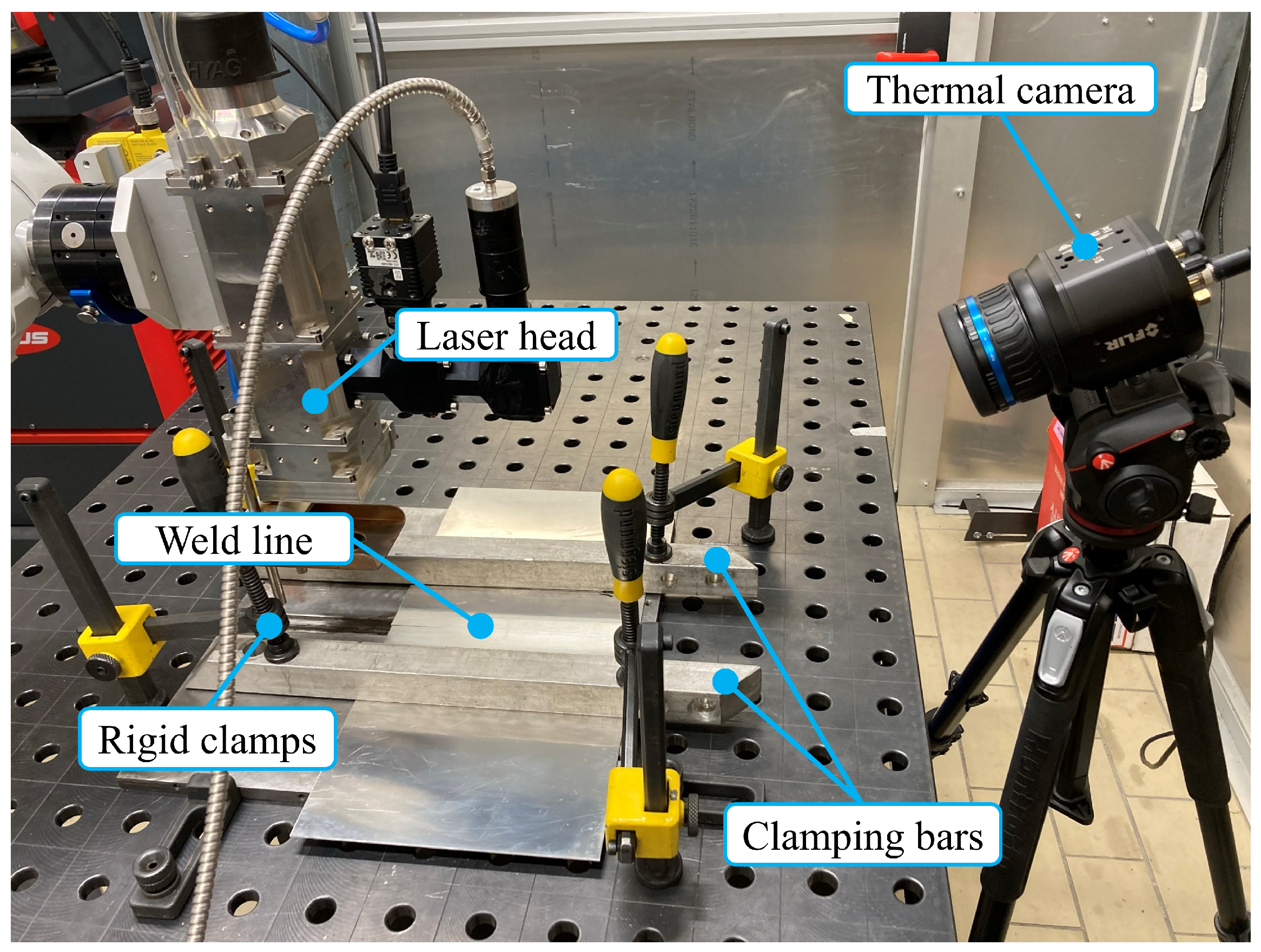
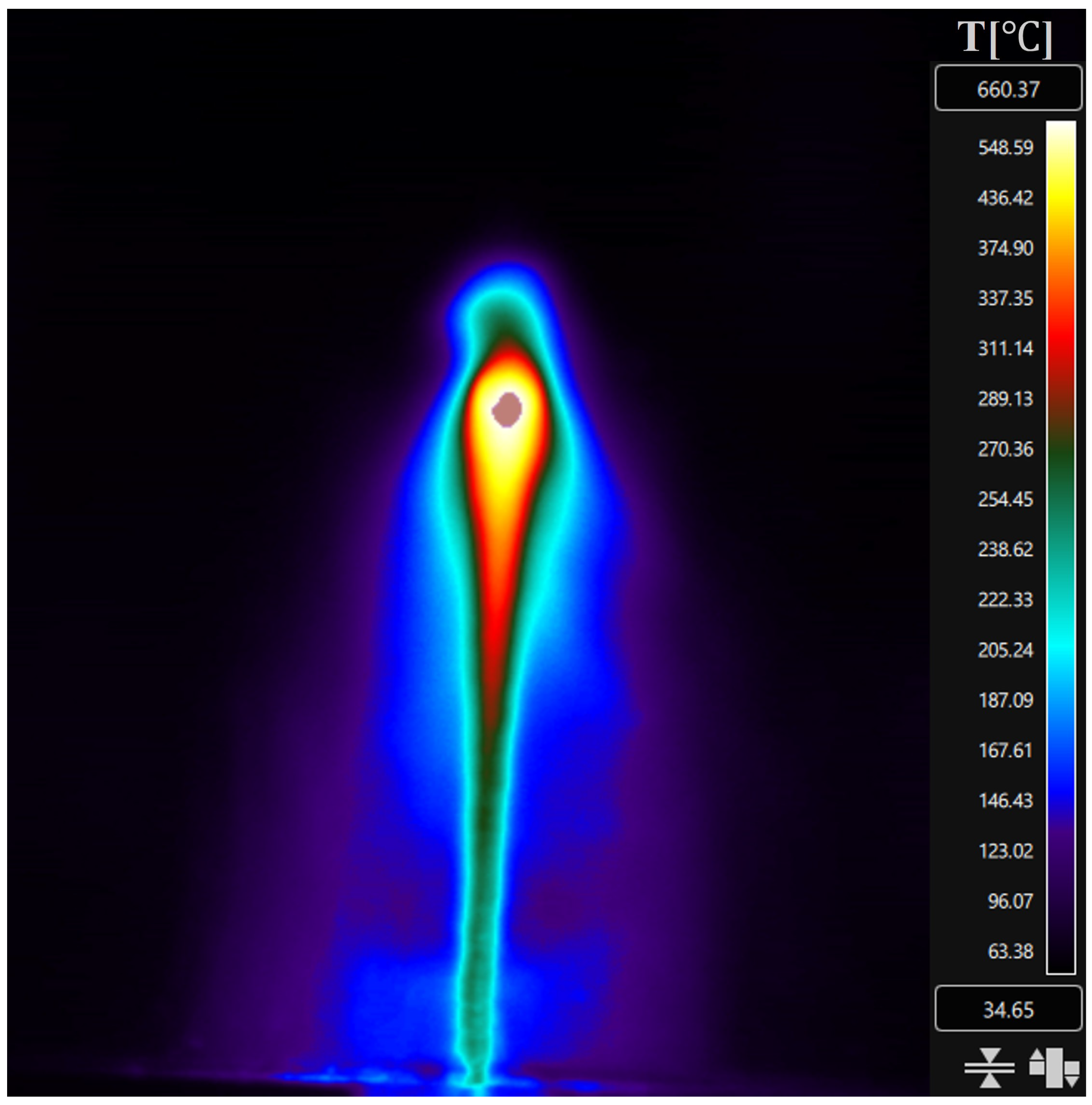
IR Camera Monitoring

A FLIR A700 microbolometric (Teledyne FLIR LLC; Wilsonville, OR, USA) infrared camera equipped with an 24 × 18 lens was used to monitor the laser welding process. This camera featured a long-wave sensor (7–14 $\mathsf{\mu }\mathrm{m}$), making it compatible with laser welding sources operating near $1\mathsf{\mu }\mathrm{m}$ wavelength. It was positioned 600 $\mathrm{m}\mathrm{m}$ from the weld seam at a 40° angle to the horizontal plane, providing an IFOV of 676 mrad. The temperature measurement range is 0–700 $°\mathrm{C}$, and the system was set at a fixed distance of 1.00 m from the specimen to ensure consistent data acquisition. For butt joint welds, the specimens were carefully oriented to provide an acceptable view and spatial resolution. Thermal data was post-processed using FLIR Research Studio 2024.07.1 software.

Calibration of the IR system is necessary because the surface thermal emissivity varies strongly with temperature. By identifying an isothermal plateau corresponding to the solid–liquid phase transition (around 650–670 $°\mathrm{C}$) and comparing it with the literature values for aluminium 6061 and 6082 alloys, the surface emissivity was set to 0.35.

To extract a thermal cycle suitable for use in the simulation, which is comparable to that obtained from the MHS model, the thermograms were analysed to identify a region located just outside the molten zone. The thermal history in this region was extracted and used as input for the IR-ITC model.

4. Experimental Results

This section presents the experimental tests and numerical simulations used to validate both the conventional and proposed modeling approaches. Comparisons focus on cross-sectional metallography, thermal distribution, and mechanical distortions.

4.1. Materials and Experimental Methodology

To demonstrate the effectiveness of the proposed approach, we have performed two laser welding experiments to acquire reference data.

The laser beam source is a diode laser (LDF4000-40, Laserline, Mülheim-Kärlich, Germany) with a maximum power of 4 kW and two wavelengths of 1020 and 1060 ± 10 nm. The welding head (OTS-5, Laserline, Mülheim-Kärlich, Germany) is mounted on a 6-axis industrial robot (IRB2400, ABB, Zurich, Switzerland) Welding is conducted on 1.5 mm-thick Al 6061-T6 plates, each measuring $150\times 200$ mm, in a butt configuration. Prior to welding, the joint area was sanded and polished to remove contaminants (grease and dirt traces) and then cleaned thoroughly with acetone. The two aluminium plates were clamped to ensure a zero-gap joint, as illustrated in Figure 6. The laser beam was oriented perpendicular to the plate surface, and the focal point was adjusted to 3 mm above the plate surface, resulting in a beam spot diameter of 1.2 mm. Neither shielding gas nor filler material was used during welding. We have set the laser power at 2800 W. The two welding experiments differ only in the welding speed: 35 and 50 ${\mathrm{m}\mathrm{m}\mathrm{s}}^{-1}$ for Sample 1 and Sample 2, respectively. The welding parameters were selected based on preliminary trials aimed explicitly at maximizing weld-induced distortions. The goal is to generate significant mechanical deformation, which is particularly challenging to predict by FEM simulations. Thus, parameter selection prioritizes distortion magnitude over weld joint quality.

To examine the joint geometry, a cross-sectional specimen was prepared by cutting through the weld zone. The samples were hot-mounted, polished to achieve a homogeneous surface finish, and then chemically etched using Keller’s reagent for metallographic analysis. The cross-sectional images of the welding zone were captured using an (optical microscope (Axiovert a1, Zeiss, Oberkochen, Germany). Subsequently, the molten pool geometry is measured using the software ImageJ 1.54g. Post-weld distortion of the aluminium sheets is assessed using a direct contact profilometer. One side of the sheet is fixed, as shown in Figure 7, and the measurement line is oriented at a 90° angle to the weld seam, positioned at the midpoint of the sheet.

4.2. Numerical Solver

Considering the complexity of the welding process and focusing on understanding the effect of heat input on mechanical distortion, the models described in Section 2.1 were numerically solved through FEM analysis. A single FEM model was employed for both samples, with varying input parameters, and simulations were carried out using SYSWELD 2024.0 software in two steps: a thermo-metallurgical simulation followed by a mechanical simulation [36,45]. Material properties and model parameters were selected according to the SYSWELD 2024.0 database. The conductive heat transfer is set to $h_c=25$ $\mathrm{W}{\mathrm{m}}^{-2} {\mathrm{K}}^{-1}$, and surface emissivity as $ϵ=0.8$.

Using the Visual-Mesh (SYSWELD 2024.0) module, mesh was defined with 54,400 8-node hexahedral linear 3D prism elements representing the solid domain; 36,544 4-node rectangular linear 2D elements to model heat exchange with the environment; and 200 1D line elements to define both the welding trajectory and reference lines.

Figure 2 provides an overview of the model, including spatial orientation, clamping positions, and Heat Affected Zone (HAZ) mesh appearance. The coordinate system is defined as follows: x-axis corresponds to the welding direction, the y-axis to the width of the weldment, and the z-axis to the direction of weld pool penetration (i.e., thickness). Mesh density was refined in thermally critical regions to ensure accuracy while maintaining reasonable computational time. Specifically, finer mesh grids of $0.25\times 0.25\times 1.0$ mm were used in the HAZ, with a transition to coarser center-concentric biased elements beyond the Fusion Zone (FZ) [8]. The Broyden–Fletcher–Goldfarb–Shanno (BFGS) algorithm was used to ensure the convergence and the stability of the numerical model computation [9].

In the same welding conditions, thinner plates are more prone to longitudinal and transverse shrinkage, as well as angular distortions due to thermal volumetric expansion and contraction during welding [46]). In FEM simulations based on small deformation theory, where strain is linearly dependent on displacement, large distortions are often underestimated. However, the interaction of large distortions (longitudinal, transverse, and bidirectional angular) leads to the buckling phenomenon. In large distortion theory, instead, strain is a nonlinear function of displacement. The nonlinear geometry option of SYSWELD 2024.0 accounts for such behavior, though some discrepancy between experimental and FEM numerical results still remains [47]. In this work, the bending optimized function of SYSWELD 2024.0 was used to improve the accuracy of distortion computation. Standard hexahedral elements are limited in accurately capturing bending kinematics. This limitation is addressed by using incompatible mode elements, which incorporate additional shape functions to better model bending behavior [48]. As a result, all solid elements, except those in the HAZ, were defined as type 2 (i.e., incompatible mode elements) to enhance the accuracy of distortion computations.

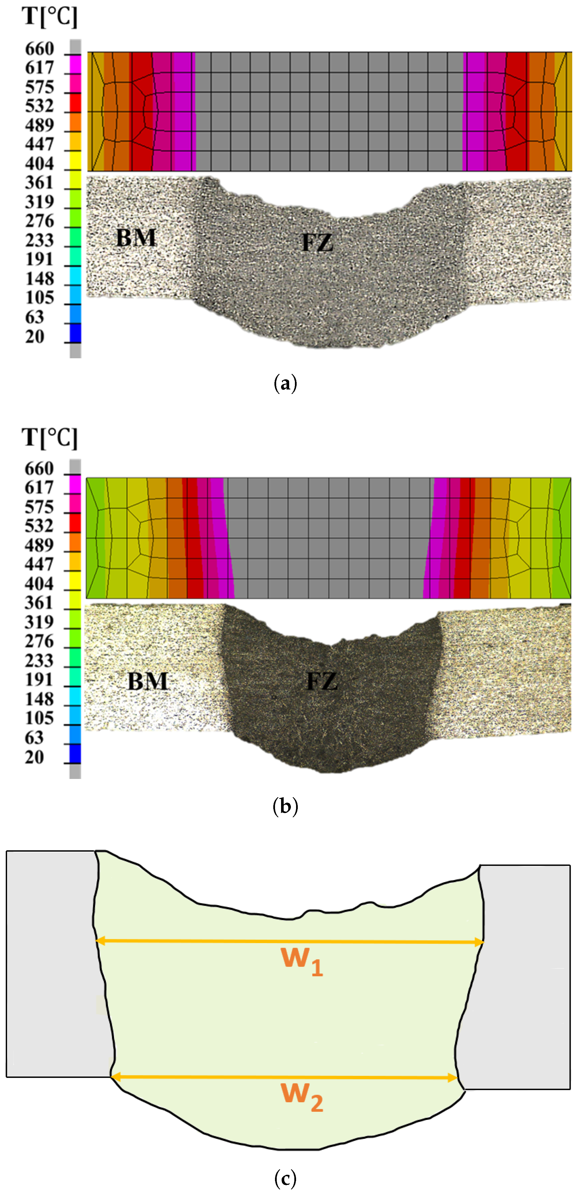
4.3. Cross-Section Comparison and Time Analysis

Figure 8 illustrates the criteria used for measuring the melt pool and presents a comparative analysis between the metallographic cross-sections of the laser-welded aluminium alloys (Sample 1 and Sample 2) and the corresponding results from MHS simulations. Both experimental and simulated results clearly display the Base Metal (BM) and Fusion Zone (FZ).

Table 1. Comparison of FEM and experimental weld pool dimensions.

Sample	FEM (mm)		Experiment (mm)
	${\mathbf{w}}_{\mathbf{1}}$	${\mathbf{w}}_{\mathbf{2}}$	${\mathbf{w}}_{\mathbf{1}}$	${\mathbf{w}}_{\mathbf{2}}$
1	3.22	3.18	3.20	3.20
2	2.65	2.30	2.64	2.29

summarizes the fusion zone dimensions obtained from the cross-sectional analysis.

The calibrated model exhibits only minor differences between the experimental and FEM results for the weld widths ${\mathbf{w}}_{\mathbf{1}}$ and ${\mathbf{w}}_{\mathbf{2}}$. In Sample 2, a smaller fusion zone is observed, which can be attributed to the lower heat input per unit length caused by the higher welding speed.

Within the scope of this study, numerical simulations based on the MHS, T-ITC, and IR-ITC approaches are carried out for Sample 1 and Sample 2.

Table 2. Breakdown of simulation workflow stages and corresponding time requirements for each modeling approach.

Stage	Task	MHS (h)	T-ITC (h)	IR-ITC (h)
Calibration MHS	Metallographic sample preparation	3.75	3.75	0.00
	Macroscopic analysis	0.25	0.25	0.00
	LOAD adjustment	0.90	0.90	0.00
	Heat Source inner radius adjustment	0.90	0.90	0.00
	Heat Source outer radius adjustment	0.90	0.90	0.00
	Heat Source height adjustment	0.90	0.90	0.00
	Efficiency adjustment	0.90	0.90	0.00
Thermal Cycle Preparation	Thermal cycle extraction and preparation	0.00	0.30	0.30
Calibration IR-ITC	LOAD adjustment	0.00	0.00	1.20
Computation Time	Thermo-metallurgical–mechanical simulation	1.50	0.40	0.00
Total		10.00	9.20	1.50

outlines the simulation workflow for each model and reports the elapsed time per single run. The calibration of the MHS model is the most time-consuming stage, requiring 10 h. Because the T-ITC model derives its thermal cycle from the calibrated MHS model, its calibration time is identical. In contrast, a single thermo-metallurgical–mechanical run for LOAD calibration in the IR-ITC approach requires only 0.4 h. Three such runs, corresponding to three trial LOAD, were sufficient to calibrate the IR-ITC model. The proposed IR-ITC method have required almost seven times less calibration time than the MHS model, leading to a total time saving of approximately 85% compared to the MHS approach.

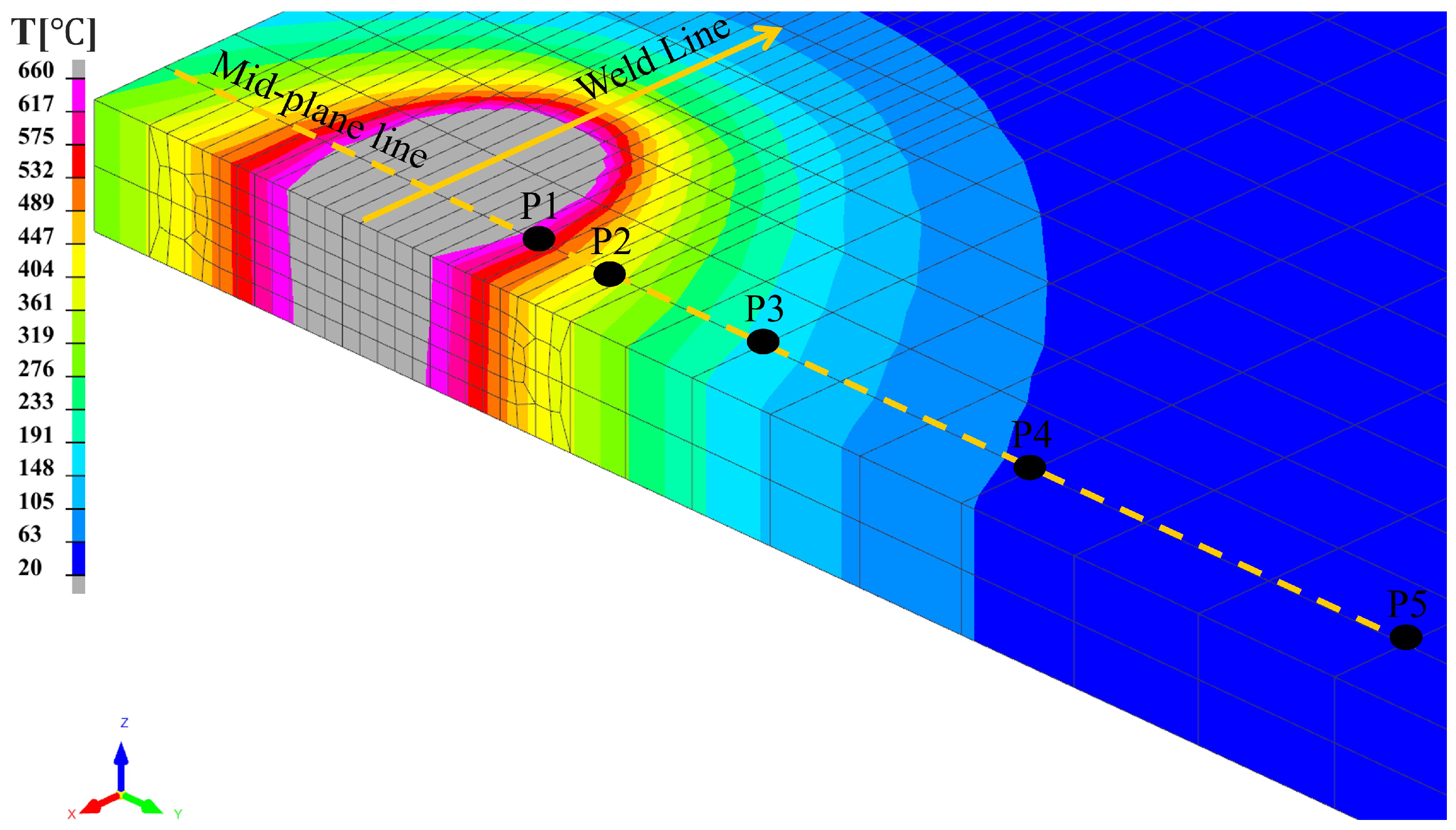
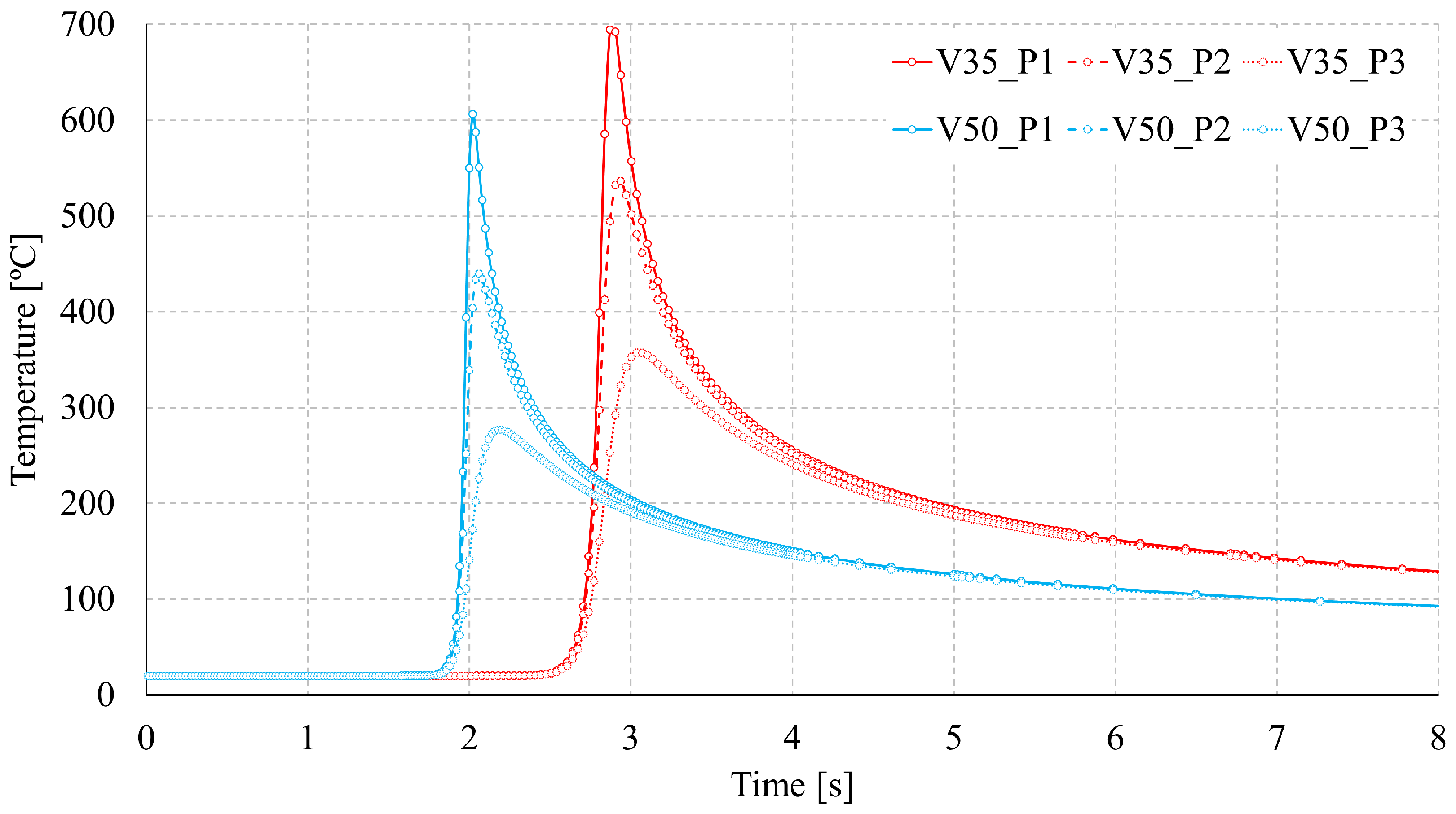
4.4. Thermal Analysis Results

Thermal distribution during the welding process was measured through thermographic monitoring. Figure 9 shows a representative frame from the thermal video captured during the experiment. The boundary of the weld pool can be identified from the temperature distribution, with the white region indicating temperatures at or above the melting point of aluminium, approximately 660 $°\mathrm{C}$. It is worth noting that temperature acquisition through an IR thermal camera relies on the knowledge of the material emissivity, which varies with its physical state. In the weld pool, the emissivity of liquid aluminium differs from that of its solid form, introducing a potential error in measuring temperature inside the weld pool. Despite this limitation, the frame in Figure 9 clearly shows the temperature gradient from the outer edges of the metal sheets (cooler, darker regions) toward the weld center (hotter, lighter), where the laser is focused (i.e., about 660 $°\mathrm{C}$). The gray region at the center represents pixel saturation due to the upper temperature limit of the IR camera. However, in this study, the primary aim is on the thermal behavior outside the weld pool, but still inside the welded joint, where emissivity is more stable and temperature measurements are considered reliable. Thermal cycles were extracted at the boundary of the molten zone (refer to Figure 4) from both the MHS simulation and the IR-guided measurements. To validate the proposed methodology, the thermal cycles for T-ITC and IR-ITC are compared with those obtained from the MHS simulation for Sample 1 and Sample 2, labeled as V35 and V50, respectively. The strong correlation between these thermal profiles, as shown in Figure 10, confirms the ability of the simulation framework to capture the thermal dynamics of the welding process accurately.

Following the procedures outlined in Section 2.3 and Section 3, the thermal cycles shown in Figure 11 were extracted from the thermal profiles in Figure 10 and subsequently imposed on the T-ITC and IR-ITC numerical models.

Addressing the spatial resolution problem, the main concern might be related to the pixel-to-mm ratio. However, to use the experimental data in the simulation, the best thing is to have a pixel-to-mm ratio at least the minimum mesh element size. This avoids additional work on retrofitting temperature value in unknown areas, but at the same time avoid to have an unnecessary performing thermal camera.

The simulation successfully captures the distinct thermal cycles observed in the two samples, accurately reflecting the different heat inputs applied during welding. These differences are consistent with observations from thermographic analysis. To investigate transverse temperature variations in different models of both samples, five common reference points (P1–P5) were selected along the mid-plane line on the top surface, as shown in Figure 12. These points are located at 1.5 mm, 2.5 mm, 4.73 mm, 8.56 mm, and 13.88 mm from the weld line. Initially, temperature variation was evaluated for the MHS model at P1, P2, and P3 by comparing thermal cycles.

Figure 13 confirms the monotonic temperature drop with increasing distance from the weld center, consistent with thermal-diffusion theory. The larger heat input in Sample 1 produces uniformly higher peak temperatures. To quantify thermo-metallurgical model fidelity, instantaneous temperatures at P1–P5 are compared with the experiment, and the average difference (Avg_Diff) is computed.

Table 3. Comparison of simulated and experimental instantaneous temperatures at five selected locations (P1–P5) for different models and samples (units in °C).

Sample	Model	P1	P2	P3	P4	P5	Avg_Diff (°C)
1	Experiment	660	532	282	118	71	–
	MHS	695	494	253	97	39	31
	T-ITC	695	521	245	69	28	35
	IR-ITC (LOAD-1)	470	344	158	49	24	124
	IR-ITC (LOAD-2)	540	404	188	55	24	90
	IR-ITC (LOAD-3)	655	506	248	70	26	32
2	Experiment	628	442	201	86	64	–
	MHS	606	404	173	56	26	31
	T-ITC	620	431	159	40	24	29
	IR-ITC (LOAD-1)	423	277	102	31	21	113
	IR-ITC (LOAD-2)	507	344	127	34	21	77
	IR-ITC (LOAD-3)	600	435	168	39	21	31

summarizes these results for all models, including IR-ITC with three LOAD options. It should be noted that the higher nodal temperatures observed in Sample 1 are due to points P1–P5 being located closer to the melt pool boundary, whereas in Sample 2, these points lie slightly farther from the fusion zone. Consequently, Sample 1 is expected to exhibit greater mechanical distortion than Sample 2. In both samples, the IR-ITC model with the narrowest LOAD (LOAD-1) gives the greatest thermal deviation; LOAD-2 shows a smaller but similar trend. In contrast, MHS, T-ITC, and IR-ITC with the widest LOAD (LOAD-3) produce comparable Avg_Diff values. Due to the minimal nodal temperature differences among these three models, significant microstructural variations are unlikely. Considering this, IR-ITC with LOAD-1 and LOAD-2 is likely to yield less accurate distortion predictions than the other models due to significant thermal deviations from experimental results and corresponding nodal temperature differences. Therefore, IR-ITC evaluated with LOAD-3 can be considered a reliable representative of both MHS and T-ITC models.

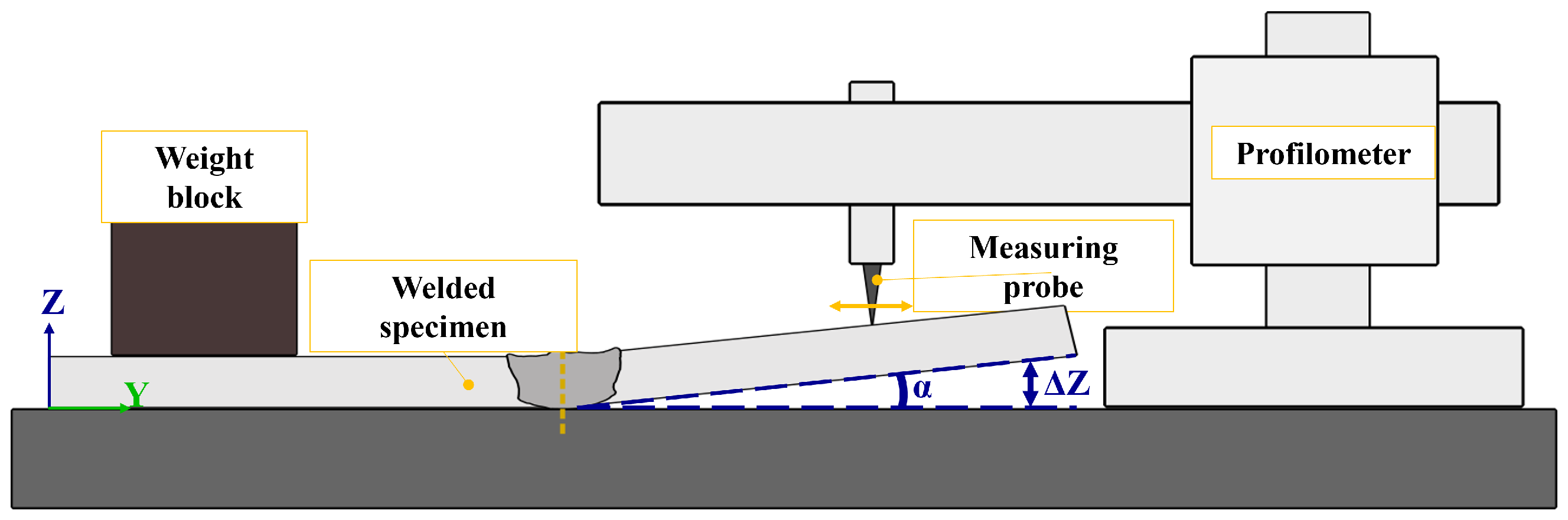
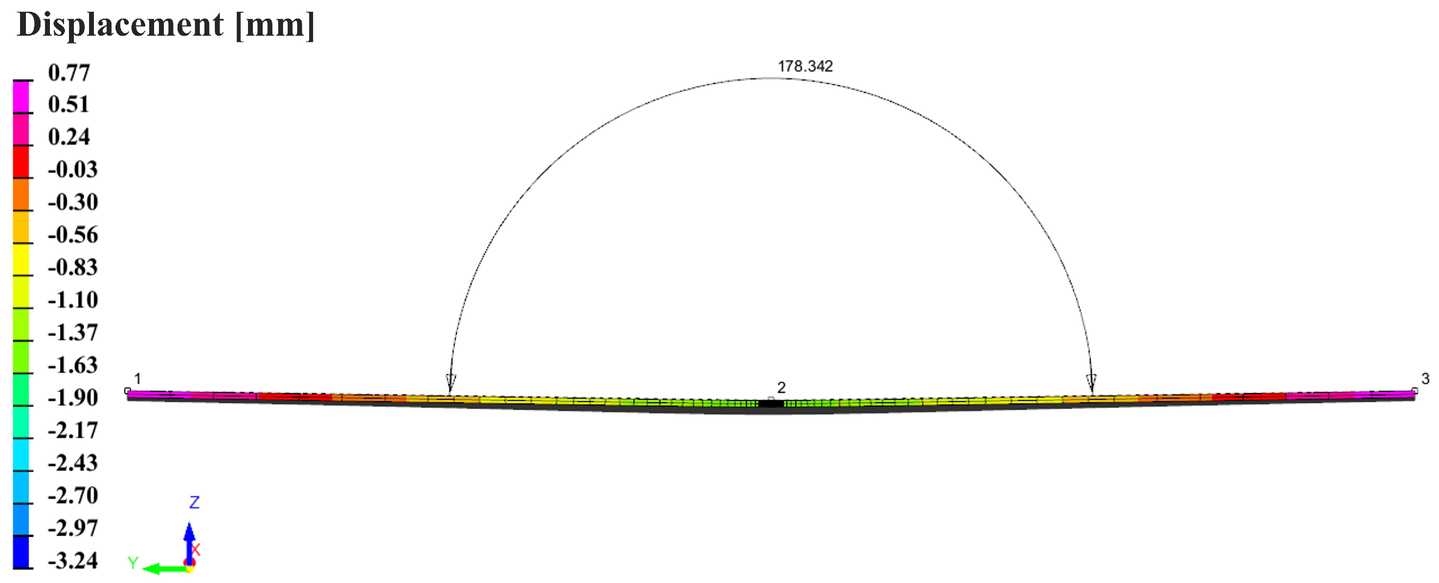
4.5. Mechanical Analysis Results

During welding, the weldment temperature is raised above the fusion temperature to ensure proper melting of the joint area. The large temperature gradient experienced during the heating and cooling stages causes significant volumetric expansion and contraction, leading to metallurgical and mechanical transformations within the material. The thermal data computed from the thermo-metallurgical simulation serve as input for the mechanical analysis, enabling the prediction of welding-induced deformations, including potential buckling behavior and residual stresses, particularly for thin aluminium alloy components. To account for these effects accurately, all numerical models were computed with nonlinear geometry effects, as recommended in [47]. In this study, the mechanical performance of the numerical models is evaluated by analyzing the estimation errors between experimental and simulated distortion angles. Figure 14 illustrates the method used to assess the distortion angle from the simulations and to compare it with the actual distortions measured using a profilometer.

At first, LOAD sensitivity test was conducted for each LOAD configuration in the IR-ITC model under identical thermal cycles derived from IR camera measurements corresponding to each sample (refer to Figure 11). The highest distortion errors are observed with the narrowest LOAD configuration in both samples, while the lowest errors occur with the widest LOAD. Specifically, for Sample 1, angular distortion errors of 0.24% and 0.18% were achieved for LOAD-2 and LOAD-3, respectively; for Sample 2, the corresponding errors are 0.32% and 0.27%. Due to the poor performance of LOAD-1 configuration in predicting distortion, its results were excluded from the final analysis. This pattern indicates that as the fusion zone (FZ) dimensions predicted by the MHS model converge with those defined by the IR-ITC LOAD configurations, the mechanical distortion discrepancies are correspondingly minimized.

Table 4. Comparison of distortion angle results between simulation models and experiments for Sample 1 and Sample 2.

Sample	Model	Angle (°)	Error (%)
1	MHS	177.98	0.15
	T-ITC	177.97	0.15
	IR-ITC	177.92	0.18
	Experiment	178.24
2	MHS	178.43	0.22
	T-ITC	178.37	0.25
	IR-ITC	178.34	0.27
	Experiment	178.82

summarizes the comparison between the numerically predicted distortion angle and the experimental measurements.

For both samples, the numerical prediction of angular distortions matches the experimental measurements, with estimation errors consistently below 0.3%. A slightly more accurate distortion estimate is obtained for Sample 1, characterized by a lower welding speed. Notably, the distortion estimation errors are comparable between the traditional simulation methods and the proposed technique. This demonstrates the efficiency of the IR-ITC approach, as it provides reasonably similar results in about 90 min, significantly faster than the over 10 h required by traditional simulation methods.

The excellent agreement between simulation and experimental results across both thermal and mechanical parameters confirms the validity of our simulation approach, whether using conventional iterative calibration or the proposed method based on thermal camera data.

5. Conclusions

This study proposes an FEM simulation approach to predict the thermal and distortion behaviors during the laser welding of thin aluminium alloy sheets. A comparative analysis between experimental observations and simulation results demonstrates strong agreement, particularly in reproducing thermal cycles and distortion profiles.

A key innovation in this work is the use of IR thermal camera data to impose thermal cycles directly in the simulation, thereby eliminating the need for calibrating a moving heat source model. This significantly simplifies the computational process and speeds up the tuning procedure. Although the predictive accuracy of the proposed simulation method may not fully match that of the MHS approach, the advantageous trade-off between significantly reduced overall workflow time and satisfactory accuracy underscores the method’s potential for practical engineering applications.

Experimental validation confirms that the proposed method achieves accuracy comparable to that of traditional simulation approaches, while reducing total time by more than 8.5 h in the present study. However, the magnitude of time and resource savings may vary depending on the model scale and other influencing parameters. This proves the efficiency of the proposed simulation approach.

It should be noted that the experimental validation in this study was limited to two welding speeds, specifically selected to induce noticeable distortion. This choice was deliberate, as our primary objective is to validate the proposed IR-ITC method under conditions known to produce significant deformation, which is particularly challenging to predict with FEM simulations accurately. However, the generalizability of our findings to a broader range of process parameters, such as different welding speeds, varying power inputs, and alternative joint configurations, still requires investigation. Future research efforts should focus on assessing the robustness and accuracy of the proposed IR-ITC methodology across a wider spectrum of welding conditions. Additionally, given that thermal cycle extraction via infrared thermography primarily relies on surface emissivity rather than being strictly material-dependent, the proposed IR-ITC method is expected to be broadly transferable to other materials and sheet thicknesses. Nevertheless, future studies should explicitly validate this methodology across different metals, alloys, and material thicknesses to fully establish its versatility and industrial applicability.

In summary, the integration of IR thermography with FEM simulations represents a meaningful advancement in the predictive modeling of laser welding processes. The proposed methodology is particularly relevant for industries such as automotive manufacturing, where it can streamline production workflows and enhance weld quality by reducing dependence on time-consuming and resource-intensive calibration procedures. Furthermore, the method is a practical engineering tool for optimizing manufacturing processes, especially in the development of lightweight and high-performance components.

References

1. Zhang, W.; Xu, J. Advanced lightweight materials for Automobiles: A review. Mater. Des. 2022, 221, 110994. [Google Scholar] [CrossRef]
2. Basile, D.; Sesana, R.; De Maddis, M.; Borella, L.; Russo Spena, P. Investigation of Strength and Formability of 6016 Aluminum Tailor Welded Blanks. Metals 2022, 12, 1593. [Google Scholar] [CrossRef]
3. Aminzadeh, A.; Silva Rivera, J.; Farhadipour, P.; Ghazi Jerniti, A.; Barka, N.; El Ouafi, A.; Mirakhorli, F.; Nadeau, F.; Gagné, M.O. Toward an intelligent aluminum laser welded blanks (ALWBs) factory based on industry 4.0; A critical review and novel smart model. Opt. Laser Technol. 2023, 167, 109661. [Google Scholar] [CrossRef]
4. Bunaziv, I.; Akselsen, O.M.; Ren, X.; Nyhus, B.; Eriksson, M. Laser Beam and Laser-Arc Hybrid Welding of Aluminium Alloys. Metals 2021, 11, 1150. [Google Scholar] [CrossRef]
5. Stavridis, J.; Papacharalampopoulos, A.; Stavropoulos, P. Quality assessment in laser welding: A critical review. Int. J. Adv. Manuf. Technol. 2018, 94, 1825–1847. [Google Scholar] [CrossRef]
6. Li, Y.; Wang, Y.; Yin, X.; Zhang, Z. Laser welding simulation of large-scale assembly module of stainless steel side-wall. Heliyon 2023, 9, e13835. [Google Scholar] [CrossRef] [PubMed]
7. Anca, A.; Cardona, A.; Risso, J.; Fachinotti, V.D. Finite element modeling of welding processes. Appl. Math. Model. 2011, 35, 688–707. [Google Scholar] [CrossRef]
8. Kik, T. Calibration of Heat Source Models in Numerical Simulations of Welding Processes. Metals 2024, 14, 1213. [Google Scholar] [CrossRef]
9. Mohan, A.; Franciosa, P.; Dai, D.; Ceglarek, D. A novel approach to control thermal induced buckling during laser welding of battery housing through a unilateral N-2-1 fixturing principle. J. Adv. Join. Process. 2024, 10, 100256. [Google Scholar] [CrossRef]
10. Chuang, T.C.; Lo, Y.L.; Tran, H.C.; Tsai, Y.A.; Chen, C.Y.; Chiu, C.P. Optimization of Butt-joint laser welding parameters for elimination of angular distortion using High-fidelity simulations and Machine learning. Opt. Laser Technol. 2023, 167, 109566. [Google Scholar] [CrossRef]
11. Yan, H.; Zeng, X.; Cui, Y.; Zou, D. Numerical and experimental study of residual stress in multi-pass laser welded 5A06 alloy ultra-thick plate. J. Mater. Res. Technol. 2024, 28, 4116–4130. [Google Scholar] [CrossRef]
12. Pyo, C.; Kim, J.; Kim, Y.; Kim, M. A study on a representative heat source model for simulating laser welding for liquid hydrogen storage containers. Mar. Struct. 2022, 86, 103260. [Google Scholar] [CrossRef]
13. Murua, O.; Arrizubieta, J.; Lamikiz, A.; Schneider, H. Numerical simulation of a laser beam welding process: From a thermomechanical model to the experimental inspection and validation. Therm. Sci. Eng. Prog. 2024, 55, 102901. [Google Scholar] [CrossRef]
14. Walker, T.; Bennett, C. An automated inverse method to calibrate thermal finite element models for numerical welding applications. J. Manuf. Process. 2019, 47, 263–283. [Google Scholar] [CrossRef]
15. Speka, M.; Matteï, S.; Pilloz, M.; Ilie, M. The infrared thermography control of the laser welding of amorphous polymers. NDT E Int. 2008, 41, 178–183. [Google Scholar] [CrossRef]
16. Bagavathiappan, S.; Lahiri, B.; Saravanan, T.; Philip, J.; Jayakumar, T. Infrared thermography for condition monitoring—A review. Infrared Phys. Technol. 2013, 60, 35–55. [Google Scholar] [CrossRef]
17. Santoro, L.; Sesana, R.; Molica Nardo, R.; Curá, F. Infrared in-line monitoring of flaws in steel welded joints: A preliminary approach with SMAW and GMAW processes. Int. J. Adv. Manuf. Technol. 2023, 128, 2655–2670. [Google Scholar] [CrossRef]
18. Santoro, L.; Sesana, R. A pilot study using flying spot laser thermography and signal reconstruction. Opt. Lasers Eng. 2025, 188, 108901. [Google Scholar] [CrossRef]
19. Sesana, R.; Santoro, L.; Curà, F.; Molica Nardo, R.; Pagano, P. Assessing thermal properties of multipass weld beads using active thermography: Microstructural variations and anisotropy analysis. Int. J. Adv. Manuf. Technol. 2023, 128, 2525–2536. [Google Scholar] [CrossRef]
20. Vasilev, M.; MacLeod, C.N.; Loukas, C.; Javadi, Y.; Vithanage, R.K.W.; Lines, D.; Mohseni, E.; Pierce, S.G.; Gachagan, A. Sensor-Enabled Multi-Robot System for Automated Welding and In-Process Ultrasonic NDE. Sensors 2021, 21, 5077. [Google Scholar] [CrossRef] [PubMed]
21. Nguyen, H.L.; Van Nguyen, A.; Duy, H.L.; Nguyen, T.H.; Tashiro, S.; Tanaka, M. Relationship among Welding Defects with Convection and Material Flow Dynamic Considering Principal Forces in Plasma Arc Welding. Metals 2021, 11, 1444. [Google Scholar] [CrossRef]
22. Zhu, C.; Cheon, J.; Tang, X.; Na, S.J.; Cui, H. Molten pool behaviors and their influences on welding defects in narrow gap GMAW of 5083 Al-alloy. Int. J. Heat Mass Transf. 2018, 126, 1206–1221. [Google Scholar] [CrossRef]
23. Filyakov, A.E.; Sholokhov, M.A.; Poloskov, S.I.; Melnikov, A.Y. The study of the influence of deviations of the arc energy parameters on the defects formation during automatic welding of pipelines. In Proceedings of the IOP Conference Series: Materials Science and Engineering, Nizniy Tagil, Russia, 24–29 February 2020; Volume 966. [Google Scholar] [CrossRef]
24. Aucott, L.; Huang, D.; Dong, H.B.; Wen, S.W.; Marsden, J.A.; Rack, A.; Cocks, A.C.F. Initiation and growth kinetics of solidification cracking during welding of steel. Sci. Rep. 2017, 7, 40255. [Google Scholar] [CrossRef] [PubMed]
25. Hong, Y.; Yang, M.; Chang, B.; Du, D. Filter-PCA-Based Process Monitoring and Defect Identification During Climbing Helium Arc Welding Process Using DE-SVM. IEEE Trans. Ind. Electron. 2023, 70, 7353–7362. [Google Scholar] [CrossRef]
26. D’Accardi, E.; Chiappini, F.; Giannasi, A.; Guerrini, M.; Maggiani, G.; Palumbo, D.; Galietti, U. Online monitoring of direct laser metal deposition process by means of infrared thermography. Prog. Addit. Manuf. 2024, 9, 983–1001. [Google Scholar] [CrossRef]
27. Razza, V.; Santoro, L.; De Maddis, M. Gradient-based image generation for thermographic material inspection. Appl. Therm. Eng. 2025, 268, 125900. [Google Scholar] [CrossRef]
28. Santoro, L.; Razza, V.; De Maddis, M. Frequency-based analysis of active laser thermography for spot weld quality assessment. Int. J. Adv. Manuf. Technol. 2024, 130, 3017–3029. [Google Scholar] [CrossRef]
29. Santoro, L.; Razza, V.; De Maddis, M. Nugget and corona bond size measurement through active thermography and transfer learning model. Int. J. Adv. Manuf. Technol. 2024, 133, 5883–5896. [Google Scholar] [CrossRef]
30. Zhang, C.; Li, X.; Gao, M. Effects of circular oscillating beam on heat transfer and melt flow of laser melting pool. J. Mater. Res. Technol. 2020, 9, 9271–9282. [Google Scholar] [CrossRef]
31. Zhou, Q.; Rong, Y.; Shao, X.; Jiang, P.; Gao, Z.; Cao, L. Optimization of laser brazing onto galvanized steel based on ensemble of metamodels. J. Intell. Manuf. 2018, 29, 1417–1431. [Google Scholar] [CrossRef]
32. Mirapeix, J.; García-Allende, P.; Cobo, A.; Conde, O.; López-Higuera, J. Real-time arc-welding defect detection and classification with principal component analysis and artificial neural networks. NDT E Int. 2007, 40, 315–323. [Google Scholar] [CrossRef]
33. Zhang, H.; Chen, Z.; Zhang, C.; Xi, J.; Le, X. Weld Defect Detection Based on Deep Learning Method. In Proceedings of the 2019 IEEE 15th International Conference on Automation Science and Engineering (CASE), Vancouver, BC, Canada, 22–26 August 2019; pp. 1574–1579. [Google Scholar] [CrossRef]
34. Sarkar, S.S.; Das, A.; Paul, S.; Mali, K.; Ghosh, A.; Sarkar, R.; Kumar, A. Machine learning method to predict and analyse transient temperature in submerged arc welding. Measurement 2021, 170, 108713. [Google Scholar] [CrossRef]
35. Bergman, T.L.; Lavine, A.S.; Incropera, F.P.; DeWitt, D.P. Fundamentals of Heat and Mass Transfer, 8th ed.; John Wiley & Sons, Inc.: Hoboken, NJ, USA, 2018. [Google Scholar]
36. Kik, T. Computational Techniques in Numerical Simulations of Arc and Laser Welding Processes. Materials 2020, 13, 608. [Google Scholar] [CrossRef] [PubMed]
37. Unni, A.K.; Vasudevan, M. Computational fluid dynamics simulation of hybrid laser-MIG welding of 316 LN stainless steel using hybrid heat source. Int. J. Therm. Sci. 2023, 185, 108042. [Google Scholar] [CrossRef]
38. Rong, Y.; Huang, Y.; Wang, L. Evolution Mechanism of Transient Strain and Residual Stress Distribution in Al 6061 Laser Welding. Crystals 2021, 11, 205. [Google Scholar] [CrossRef]
39. Tian, X.; Liao, J.; Cheng, P.; Ling, Y. Element Simulation of Welding Residual Stresses and Distortion in 5083 Incorporating Metallurgical Phase Transformation. In Proceedings of the 2017 International Conference on Applied Mathematics, Modeling and Simulation (AMMS 2017), Shanghai, China, 26–27 November 2017; Atlantis Press: Dordrecht, The Netherlands, 2017; pp. 164–168. [Google Scholar] [CrossRef]
40. Schieck, B.; Stumpf, H. Deformation analysis for finite elastic-plastic strains in a lagrangean-type description. Int. J. Solids Struct. 1993, 30, 2639–2660. [Google Scholar] [CrossRef]
41. Lima, T.R.; Tavares, S.M.; de Castro, P.M. Residual stress field and distortions resulting from welding processes: Numerical modelling using Sysweld. Ciência Tecnol. Dos Mater. 2017, 29, e56–e61. [Google Scholar] [CrossRef]
42. Kik, T. Heat Source Models in Numerical Simulations of Laser Welding. Materials 2020, 13, 2653. [Google Scholar] [CrossRef] [PubMed]
43. Battista, F.R.; Ambrogio, G.; Giorgini, L.; Guerrini, M.; Costantino, S.; Ricciardi, F.; Filice, L. Prediction of the keyhole TIG welding-induced distortions on Inconel 718 industrial gas turbine component by numerical-experimental approach. Int. J. Adv. Manuf. Technol. 2024, 134, 4593–4608. [Google Scholar] [CrossRef]
44. Vargas, J.A.; Torres, J.E.; Pacheco, J.A.; Hernandez, R.J. Analysis of heat input effect on the mechanical properties of Al-6061-T6 alloy weld joints. Mater. Des. (1980–2015) 2013, 52, 556–564. [Google Scholar] [CrossRef]
45. Marques, E.S.V.; Silva, F.J.G.; Pereira, A.B. Comparison of Finite Element Methods in Fusion Welding Processes—A Review. Metals 2020, 10, 75. [Google Scholar] [CrossRef]
46. Long, H.; Gery, D.; Carlier, A.; Maropoulos, P. Prediction of welding distortion in butt joint of thin plates. Mater. Des. 2009, 30, 4126–4135. [Google Scholar] [CrossRef]
47. Vinoth, A.; Sivasankari, R. Numerical Simulation Studies in Tungsten Inert Gas Welding of Inconel 718 Alloy Sheet. J. Mater. Eng. Perform. 2024. [Google Scholar] [CrossRef]
48. Kožar, I.; Rukavina, T.; Ibrahimbegović, A. Method of Incompatible Modes—Overview and Application. Građevinar 2018, 70, 19–29. [Google Scholar] [CrossRef]
Figure 1. A 3D Gaussian truncated conical heat source model.
Metals 15 00830 g001
Figure 2. Finite element model schematic and clamping positions.
Metals 15 00830 g002
Figure 3. Selected mesh elements (LOAD) heated by MHS.
Metals 15 00830 g003
Figure 4. Thermal cycle extraction node positions from the moving heat source models: (a) Sample 1, (b) Sample 2.
Metals 15 00830 g004
Figure 5. Three different LOAD configurations for the IR-ITC method.
Metals 15 00830 g005
Figure 6. Welding setup and thermal camera.
Metals 15 00830 g006
Figure 7. Profilometer measurements set-up.
Metals 15 00830 g007
Figure 8. Comparison of numerical and experimental melt pool morphology: (a) Sample 1, (b) Sample 2, (c) fusion zone measurement criteria.
Metals 15 00830 g008
Figure 9. Thermography map highlighting the weld pool.
Metals 15 00830 g009
Figure 10. Comparison of experimental and numerical thermal cycles.
Metals 15 00830 g010
Figure 11. Comparison between the extracted thermal cycles from the MHS model (T-ITC) and the IR-guided thermal cycles (IR-ITC) for Sample 1 and Sample 2.
Metals 15 00830 g011
Figure 12. Selected points (P1–P5) along the mid-plane line used for quantitative thermal analysis.
Metals 15 00830 g012
Figure 13. Temperature evolution at points P1–P3 along the central cross-section for Sample 1 and Sample 2.
Metals 15 00830 g013
Figure 14. Distortion angle measurement from numerical models.
Metals 15 00830 g014