Abstract
The experimental tests needed for the estimation of the fatigue limit generally require extensive time and many specimens. A valid but not standardized alternative is the thermographic analysis of the self-heating phenomenon. The present work is aimed at using Infrared thermography to determine the fatigue limit in two kinds of Ti-6Al-4V samples obtained by hot rolling: (1) with the standard dog-bone shape (unnotched specimen) and (2) with two opposed semicircular notches at the sides (notched specimen). Uniaxial tensile experiments are performed on unnotched samples, and the surface temperature variation during loading is monitored. The stress corresponding to the end of the thermoelastic stage gives a rough indication of the fatigue limit. Then, fatigue tests at different sinusoidal loads are performed, and the thermographic signal is monitored and processed. The results obtained using lock-in thermography in dissipative mode, e.g., analyzing the second harmonic, showed a sudden change in slope when the applied stress exceeded a certain limit. This slope change is related to the fatigue limit. In addition, the ratio between the fatigue limits obtained for notched and unnotched specimens, e.g., the fatigue strength reduction factor, is consistent with literature values based on the selected geometry.
1. Introduction
The fatigue limit is the most meaningful parameter summarizing the fatigue performance of materials, introduced for engineering purposes of design based on experimental data. According to [1], it identifies a transition in the mechanical behavior of metallic materials between high-cycle fatigue (HCF) and very high-cycle fatigue (VHCF). The experimental tests needed for its estimation, e.g., the Staircase method (ISO 12107 standard [2]), usually require extensive time and many specimens to ensure repeatability and consistency. A valid alternative to this standardized method to estimate the fatigue limit is the Infrared (IR) thermographic approach. IR thermography is a non-contact, full-field technique for measuring the surface temperature of a body. Heat dissipation is not, by nature, an indicator of fatigue damage because temperature variations can be observed in a specimen cyclically loaded below the fatigue limit, due to non-damaging anelastic dissipative phenomena [3]. However, when the transition from anelastic to inelastic strains happens, heat dissipation becomes more significant. For this reason, over the last years, heat dissipation has been accepted as an appropriate damage indicator of the material [4].
Applications of IR thermography to fatigue limit estimation were proposed several years ago by Luong [5] and La Rosa and Risitano [6] based on empirical observations. The approach relies on analyzing the surface temperature during a constant amplitude fatigue test. The average temperature vs. time trend exhibits an initial transient followed by a plateau, asymptotically tending to a stabilized temperature ΔTstab, which is characteristic of the tested material, the stress amplitude, and the stress ratio, provided that the applied frequency is sufficiently high to achieve adiabatic conditions.
IR thermography was used to process fatigue data of metallic materials while analyzing other thermal quantities beyond ΔTstab, such as the initial slope over cycles dT/dN at the beginning of the fatigue loading [7,8], the Discrete Fourier Transform (DFT) of the first harmonic or thermoelastic signal [9,10] and of the second harmonic or dissipative signal [11,12,13,14,15], the dissipated heat per cycle [16], and the dissipative energy density [17,18,19].
Teng [20], Zaeimi et al. [21], Wei et al. [22], and Vergani et al. [23] reviewed these and other approaches to discuss the possibility of applying them to the estimation of the fatigue limit, both in metallic and composite materials. Regardless of the IR thermographic quantity analyzed, the procedure for the rapid estimation of the fatigue limit considers monitoring the IR response during blocks of fatigue cycles at progressively increasing load and plotting it as a function of this applied load. The data typically have a bilinear trend. The theoretical approach based on thermodynamic equations proposed by Yang et al. [17] evidences that the first regime is related to fatigue anelastic effects, which do not contribute to damage accumulation. On the other hand, the second regime is linked to inelastic effects arising from micro-plasticity within the material. This second regime is the primary cause of fatigue damage and, ultimately, fatigue fracture. The breakup point corresponding to the change in slope identifies a stress that is the thermographic estimation of the fatigue limit. This point was also named σD [24], where the subscript D stands for damage. It corresponds to the stress at which the thermographic measurements can identify a thermal variation between anelastic and inelastic phenomena due to irreversible fatigue damage, or, in other words, damage initiation.
However, steels can also experience non-linear trends of the IR quantity as a function of the applied stress. Some authors addressed this problem of thermal data interpolation by suggesting different techniques to identify univocally the fatigue limit. Table 1 shows some techniques proposed in the literature, based on the analysis of the 1st and 2nd regimes of the available IR thermal quantities.

Table 1.
Literature techniques for IR thermographic data interpolation for the identification of the fatigue limit. The techniques identify the fatigue limit as the transition point between two thermal regimes, e.g., below and above the fatigue limit.
Interpreting thermographic data requires expertise in both material science and IR thermographic techniques. Indeed, many factors can influence the thermographic signal, such as surface finishing, which include roughness and defects that affect heat dissipation. These are especially important in the case of additively manufactured coupons [31,32], specimen geometry with stress concentration from notches [26], and loading conditions [33,34], e.g., stress ratio, frequency, etc.
The present study aims to apply IR thermography as a rapid tool to estimate the fatigue limit of a titanium alloy. Titanium and its alloys are particularly challenging from the thermographic viewpoint because of their low thermal dissipation, e.g., their thermal conductivity is significantly lower than that of steel or aluminum (~6–7 vs 40–60 and 150–250 W/m·K, respectively [35,36]). Indeed, this causes localized heat to build up slowly or not propagate efficiently during cyclic loading. As a result, IR cameras may fail to detect the small temperature gradients or thermal plateaus during fatigue cycling. In addition, the surface oxide layer of titanium alloys can affect its emissivity, which can mask the real thermal signals associated with fatigue processes.
Together with the challenges in the thermographic signal processing and the methodology to properly identify the fatigue limit, the paper also discusses the effect of a notch and the roughness at its fillet from the perspective of possible applications of the thermographic method on real components.
2. Materials and Methods
The material object of this study is the Ti-6Al-4V alloy. After lamination, plates underwent a thermal treatment at 800 °C for 1h, and then, they were water-tempered.
Residual stress measurements were performed on coupons in the regions using an X-Ray Diffractometer AST X-Stress 3000 G2 (by Stresstech Oy Co., Vaajakoski, Finland) with a collimator of 2 mm diameter, a Ti-target tube, a single-point exposure time period of 90 s, and 5 measurement points for diffraction angle. The resulting residual stresses along the loading direction of the specimens are −55 ± 11 MPa.
Figure 1 shows the geometries of the two specimen types, cut from the laminated plates by EDM (Electrical Discharge Machining). The first geometry (S-specimen, Figure 1a) was selected based on the ASTM E8-E8M standard. Since the investigated area is the middle portion of the specimen, where there are no nominal notches, its results will be considered as a reference for the material’s properties. On the other hand, the second geometry (N-specimen, Figure 1b) was designed with opposite semicircular notches, similar to the work by Curà et al. [26]. The corresponding stress concentration factor value is as follows [37,38]:
where r is 1 mm, i.e., the groove radius, and H is 8 mm, i.e., the specimen width. The resulting from Equation (1) is 2.27.
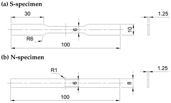
Figure 1.
Dimensions of the standard (a) and notched (b) specimens (unit: mm).
All specimens were coated with a spray black matte paint to avoid environmental reflections.
Table 2 shows the static properties from tensile tests following the ASTM E8/E8M standard on S-specimens in displacement control (0.8 mm/min) using the electro-mechanical MTS RT-100 testing machine. The corresponding stress–strain curve is shown in Figure 2a. During the tensile test, the central part of the specimen (region of interest (ROI)) was thermographically monitored using an IR camera (Model Cedip-FLIR Titanium by FLIR Systems, Täby, Sweden) with an InSb sensor having a Noise Equivalent Temperature Difference (NETD) equal to 25 mK. Figure 2b,c show an example of the combination of mechanical and thermal information. The specimen experiences an initial cooling relative to the initial room temperature T0 due to the thermoelastic phenomenon (i.e., the thermoelastic effect), followed by a progressive self-heating up to the failure with the final sudden release of thermal energy, as visible from the thermograms in Figure 2e.
Table 2.
Static properties of the tested Ti-6Al-4V.
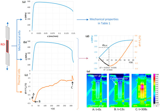
Figure 2.
Scheme of the mechanical and thermal information from the static test on S-specimens: (a) stress–strain curve; (b) stress–time curve; (c) temperature variation–time curve; (d) combined stress–temperature variation curve at the beginning of the test; and (e) example of thermograms. The temperature is averaged over the region of interest (ROI).
Heat transfer to and from the environment can affect the surface temperature of metallic materials during static tests, e.g., the static test is not adiabatic. However, it typically follows three stages. Initially, the loaded body undergoes initial cooling due to the elastic stress field, whose governing thermoelastic law was proposed by Lord Kelvin. Then, in the second stage, the majority of the crystals are elastically stressed, with a fraction plastically deformed; the surface temperature deviates from linearity until reaching a minimum value. Finally, all crystals are plastically deformed in the third stage, becoming sources of heat generation due to the irreversible dislocation motion [39].
The end of the thermoelastic stage can be identified from the linear regression of the temperature variation vs time data (see Figure 2d). Thermal data are added to the regression until the determination coefficient R2 is higher than 98.5%. R2 would decrease if further data were added to the regression, meaning that its derivative as a function of time will always be negative. According to [40,41], the stress corresponding to the end of this linear trend is an estimation of the damage stress σD,st. This is typically smaller than the yield stress, and it identifies the beginning of the irreversible damage. These authors relate σD,st to the fatigue strength, even if this estimation comes from an experimental measurement collected from static tests.
Since the mechanisms leading to static and fatigue damage in a metallic material are not identical, the static procedure to estimate the damage stress is an unresolved issue. When a cyclic load is applied, the surface temperature of the specimen evolves exponentially (phase 1), reaching a plateau that is proportional to the applied load (phase 2). Near the failure, the temperature rises locally where the crack propagates (phase 3) [6]. Therefore, the thermal signal can give information not only when a long crack propagates at the surface but for the entire duration of the fatigue test.
The thermographic estimation of the fatigue limit or damage stress σD with fatigue tests is more reliable than with static tests, and it is easier to correlate these thermographic outputs with standard fatigue data. In the present study, the value of σD,st is collected with these purposes: (1) select the testing parameters of the stepwise fatigue tests and (2) compare it to the thermographic estimation of the fatigue limit from the stepwise tests, presented in the Results section. σD,st is typically associated with the fully reversed fatigue limit at stress ratio R = −1 [41], where R = σmin/σmax.
Sinusoidal fatigue tests are performed with a stress ratio R = 0.1 and frequency of 15 Hz, progressively increasing the stress amplitude, e.g., stepwise tests. For these types of tests, the following are the main parameters that are selected:
- -
- The initial stress amplitude . The thermographic literature suggests selecting this stress as 60–70% the expected fatigue limit [34], or 20–30% of the [42], in order to have sufficient data below the fatigue limit itself. Similarly, one can also select the initial maximum stress , considering that = 0.45 at R = −1. The selected values of and are as follows:
- ○
- for the unnotched S-specimens, 81 MPa and 180 MPa;
- ○
- for the notched N-specimens, 49.5 MPa and 110 MPa.
- -
- The step of the stress amplitude, , that is the stress increment with respect to the maximum stress. Reference [34] suggests using 10% as the expected fatigue limit; hence, the values of 9 MPa ( 20 MPa) and 6.75 MPa ( 15 MPa) are selected.
- -
- The number of cycles for each loading block. This choice depends on the possibility of reaching a stabilized temperature ( or corresponding to the equilibrium condition between generated and dissipated heat. On the other hand, should be selected to avoid accumulating excessive damage in each block, especially at high loads. For the considered alloy, 5000 cycles were sufficient based on some initial tests and the literature, which suggest a range between 1000 [43] and 20,000 [44] cycles.
The fatigue tests are performed with the servo-hydraulic MTS Landmark testing machine with a load cell of 25 kN capacity. Figure 3 shows a scheme of the experimental setup. The specimen’s surface is thermally monitored during the tests with the IR camera FLIR Titanium, connecting the load cell to the lock-in module. This allows for analyzing the self-heating during the loading cycles, e.g., thermal signals on the specimen’s surface are collected together with the forcing loading signal. This signal processing is performed with the software Altair LI by FLIR Systems (v.5.90.002, Täby, Sweden), allowing for the estimation of the first and second harmonics of the temperature signal, commercially called E-mode and D-mode, respectively. When a metallic material is subjected to cyclic loading within the elastic range and under adiabatic conditions, the surface temperature is influenced by the thermoelastic effect. This effect results in temperature modulation at the same frequency as the applied load, corresponding to the first harmonic. As irreversible damage begins to occur and heat is dissipated, additional heat source terms and higher harmonics come into play. Enke [45] proposed that this irreversible heat introduces a modulation in the temperature fluctuations, with a significant peak occurring at twice the loading frequency. A theoretical basis for this was provided by Meneghetti and Ricotta [46]. The second harmonic of thermographic signal is correlated to the dissipated energy [13] and also finds its theoretical basis in the works of Yang et al. [17] and Huang et al. [19], as previously mentioned in the Section 1.
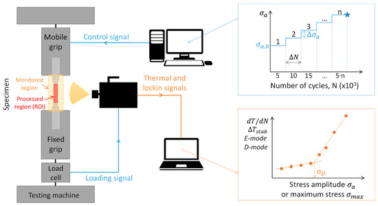
Figure 3.
Schematic of the experimental setup for the stepwise tests to monitor the self-heating.
Stepwise tests on a single specimen imply the hypotheses of steady-state heat conduction and no influence of external convection or radiation on the thermal trends, as well as limited cumulated damage generated during each loading block with respect to the following one. Indeed, given the limited number of cycles needed to obtain the results, the cumulative damage to the specimen can be considered negligible [6].
The resolution of the thermal camera is 5.2 pixel/mm. One ROI is selected for the S-specimens, e.g., the whole central portion, as schematized in Figure 3. Additionally, for the N-specimens, two small ROIs of 2 × 2 pixels are placed at the edges of the notch. This is because there is an equal likelihood of detecting damage initiation at both notch roots.
Tests are carried out until the specimen’s failure. The acquisition frequency of the thermal camera is 63 Hz, selected to not be a multiple of the loading frequency and to obtain enough data to describe the sine wave.
The first and last 1000 cycles of each loading block are recorded using the thermal camera. In particular, the first 1000 cycles allow for determining the thermal evolution , while the last 1000 cycles are used to estimate the stabilized temperature , the first harmonic E-mode, and the second harmonic D-mode. The trends of these four parameters are collected as a function of the applied stress amplitude or the maximum stress during each block. The resulting trend is typically bilinear, and the crossing point corresponds to the stress for damage initiation or fatigue strength of the material.
The relationship between unnotched and notched specimens under fatigue loading is expressed through the fatigue strength reduction factor , which is related to :
where is the notch sensitivity that can be estimated through empirical equations, such as the following ones by Peterson [47] (Equation (3)) or by Neuber [48] (Equation (4)):
Here, is the root radius of the notch, e.g., 1 mm, and and are material constants function of , i.e., the ultimate strength of alloy, which is also connected to the grain size [49]. For steels, some empirical formulas have been proposed in the literature for , such as Equation (5) from [50,51] and Equation (6) from [52]:
Through Equations (5) and (6) and Peterson’s formula in Equation (3), the estimations of are 1.94 and 2.00, respectively.
Similarly, the estimation of for steels is given by [52]:
obtaining a of 1.86.
3. Results
The post-processed thermal data in terms of , and E-mode did not show a bilinear trend as a function of applied stress. Examples of these plots are shown in Appendix A (see Figure A1 for an S-specimen and Figure A2 for an N-specimen). In some cases, only the last blocks near the specimen’s failure showed an increase in the processed signal; however, this is not likely related to the fatigue limit, but rather to the final unstable failure mechanisms.
On the other hand, the trend of the D-mode shown in Figure 4 is more promising, even though it is clearly not bilinear.
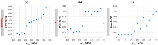
Figure 4.
Trends of the D-mode as a function of the maximum applied stress for (a) an S-specimen; (b) the left side of the notch for an N-specimen; and (c) the right side of the notch for an N-specimen.
Hence, deeper post-processing is necessary to identify the thermographic estimation of the fatigue limit. Among the different procedures suggested in the literature (see Table 1), the threshold method by De Finis et al. [28] is particularly suitable for the obtained data points. It considers these steps:
- (1)
- Calculate the average D-mode value for each ROI:where m is the total number of pixels of the ROI and is the value of the D-mode estimated with the software Altair LI in each pixel.
- (2)
- Plot as a function of the applied stress amplitude or of the maximum stress . Figure 4 shows the D-mode trends for S- and N-specimens at the different ROIs.
- (3)
- Fit the first three data points using a linear regression. This is the starting point of an iteration over the applied loading blocks. Let us consider that j is the variable spanning the loading blocks, e.g., ranging from 0 to n-3, where n is the total number of blocks. The initial value of j is 0.
- (4)
- Calculate the residuals, the standard deviation of the sample S, and the threshold value 6S, corresponding to extreme rare events. Specifically, 1S (one standard deviation) encompasses roughly 68% of the data, 2S captures about 95%, 3S includes around 99.7%, and 6S aims for near-perfect accuracy, with 99.9999998% of the data falling within its range [53];
- (5)
- If the j + 1 residual is equal or below the 6S threshold, repeat the iteration from Step 3, adding one additional data point to the fitting, e.g., j = j + 1. Else, if the j + 1 residual is above the 6S threshold, it is the thermographic estimation of the fatigue limit (or damage stress) .
For the sake of clarity, Figure A3 in Appendix B reports a flowchart of the procedure with some subfigures describing these iterative steps for the example of the S-specimen in Figure 4.
This procedure is followed for both the S- and N-specimens to process their two ROIs at the left and right sides of the notch. Figure 5 shows two examples of the identification of the fatigue limit for the S- and N-specimens. For all the tested N-specimens, the fatigue limit at the left side and at the right side coincided, e.g., , even though the trends of the residuals were different between the two ROIs (see Figure 5b,c). This difference between residuals can be due to the asymmetric generation of heating at the two notches, induced by a different distribution of initial defects and roughness at the side surface of the specimens.
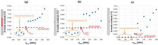
Figure 5.
Trends of the D-mode residuals as a function of the maximum applied stress for (a) an S-specimen; (b) the left side of the notch for an N-specimen; and (c) the right side of the notch for an N-specimen.
Table 3 summarizes the thermographic measurement results, averaged over three tests performed for each specimen’s geometry. The table also includes the standard deviation of the sample. For the S-specimens, it is extremely limited, suggesting that the thermographic method is robust. However, the standard deviation for the N-specimens shows higher variability due to the small processed ROIs and to the presence of stress and thermal gradients. Since the confidence bounds do not intersect, the two σD differ statistically.
Table 3.
Summary of the average and standard deviation values of the thermographic estimations of the fatigue limits, obtained for stress ratio R = 0.1.
Figure 6 and Figure 7 show images of the fracture surfaces collected with a Scanning Electron Microscope (SEM), with some details of crack origins at the surfaces. In the case of the S-specimens, multiple cracks originated at the surface cut via EDM (see Figure 6b and the related details in Figure 6c–e). This is due to the roughness of the surface, which was not polished to better understand the effect of the finishing on the thermal signal and, ultimately, on fatigue life. Surface roughness is one of the main factors that influences fatigue life because weak microstructural defects can act as stress concentrators, leading to multiple crack initiation sites. The identification of multiple cracks occurring from the side surface reveals that the material is susceptible to distributed and relatively uniform damage through the thickness, according to the thermal camera view. The cracks propagated along different planes and then generated a common front when coalescence occurred in multiple sites (Figure 6c–e). The resulting front is straight and has similar features on the two sides of the specimen, leading to unstable propagation at the middle portion.
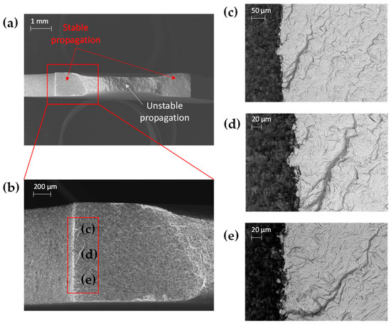
Figure 6.
SEM images of the fracture surface of an S-specimen: (a) whole fracture surface; (b) magnification at the left side; and (c–e) details of crack initiations in the regions identified in (b). Images (c,d,e) were collected using backscattered electrons.
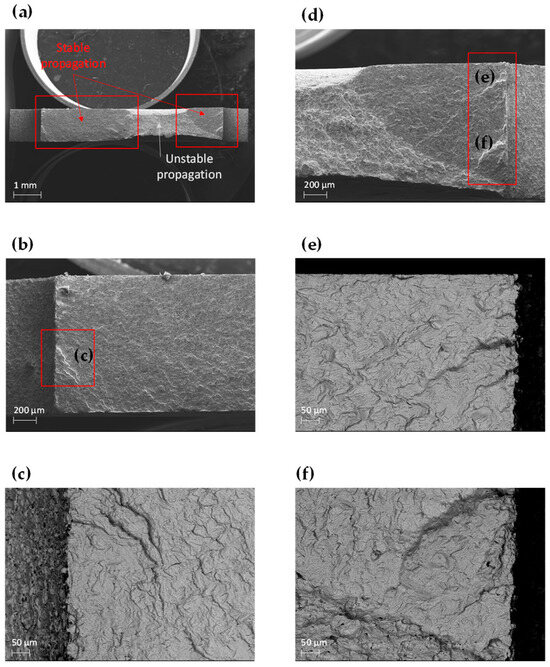
Figure 7.
SEM images of the fracture surface of an N-specimen: (a) whole fracture surface; (b) magnification at the left side; (c) details of crack initiation; (d) magnification at the right side; and (e,f) details of crack initiations. Images (c,e,f) were collected using backscattered electrons.
N-specimens also experienced propagation from multiple initiation sites at the surface. The example in Figure 7 shows that the roughness effect could generate non-straight fronts, such as in the case of the right side (see Figure 7d) due to regions where a crack was predominant (details in Figure 7e,f). This micro-mechanical behavior related to the roughness justifies the difference between different thermal signals at the two notch roots, as shown in Figure 5b,c.
4. Discussion
Despite the challenging post-processing of the thermal signal, the obtained results (Figure 5) suggest that the second harmonic or D-mode allows for the estimation of the fatigue limit. Few works relate the thermographic signal and the fatigue limit of titanium alloys in the literature. Most of them [31,54,55,56] report that the second harmonic is efficient when dealing with Ti-6Al-4V, such as in the present case.
For instance, regarding unnotched Ti-6Al-4V specimens that underwent a similar thermal treatment, Matsunaga et al. [54] identified reversible and irreversible temperature components related to thermoelastic effects and plastic deformation, respectively. They evidenced the possibility of estimating the fatigue limit through the second harmonic of the lock-in signal and the irreversible dissipated energy. They found good agreement with the fatigue limit estimated with conventional fatigue tests at various stress ratios (R = −1, 0, 0.3). In addition, their fatigue limit was 260 MPa at R = 0, consistent with the results of the present study (Table 3).
Similarly, Brot et al. [55] analyzed the self-heating in terms of the second harmonic under fatigue loads of Ti-6Al-4V specimens produced with Laser Power Bed Fusion (LPBF), with an almost elastic and perfectly plastic behavior. They tried to identify the sensitivity of the thermographic signal on the microstructure and the porosity of five material grades but underlined that only a tensile pre-strain can enhance the thermographic signal. Also, Bustos et al. [31] analyzed wrought and additive-manufactured Ti-6Al-4V specimens, as built and HIPed, discussing the effect of the surface roughness on the second harmonic thermal signal and supporting the applicability of these rapid thermographic methods for the estimation of the fatigue strength.
Akai et al. [56] studied the applicability of the thermographic method based on the mean temperature and the dissipated energy through the second harmonic. They underlined that the dissipated energy measurements were difficult because few significant changes were observed as a function of the stress amplitude. They attributed this thermal behavior to the crystal structure displaying different deformation and high vibration absorption properties.
This comparison with the literature data suggests that the thermographic analysis of titanium alloys subjected to fatigue self-heating is not straightforward and is a function of different microstructural factors. Indeed, it is worth noting that the surface finishing, grain orientation, and lamination-induced residual stresses can influence the fatigue behavior of this alloy, and they are reflected in the recorded thermographic signals. They can induce earlier irreversible damage and self-heating evidenced in the second harmonic, meaning a reduced fatigue limit. The microstructure types, such as phase distribution and grain morphology, play a role in determining the high-cycle fatigue performance of Ti-6Al-4V. Indeed, the α grain size in equiaxed microstructure or α lamellar width in lamellar microstructure has a considerable influence on the HCF strength. Wu et al. [57] underlined that the HCF strengths of different microstructures decrease in the order of bimodal, lamellar, and equiaxed microstructure. In addition, the HCF strength declines with an increase in either α grain size or α lamellar width. Specifically, for the lamellar microstructure, the fatigue limit is around 235 MPa under axial loading, indicating a significant reduction in fatigue strength compared to the bimodal microstructure. The lamellar microstructure, while offering certain mechanical advantages, may compromise fatigue resistance, making it less suitable for applications subjected to high-cycle loading conditions.
Together with the roughness and microstructure effects, another interesting result worth discussing refers to the notch effect. The ratio of σD,S to σD,N (Table 3) is the thermographic estimation of the fatigue strength reduction factor:
This value aligns well with the theoretical one, e.g., and , respectively, for Peterson’s and Neuber’s formulations, as given in the Section 2. The thermographic estimation of is lower than and of −14% and −18%, respectively.
It is likely that the presence of small compressive residual stresses, e.g., −55MPa, along the loading direction should minimally affect the fatigue limit. Indeed, residual stresses tend to relax up to 50% their initial values, especially during the first fatigue cycles, as evidenced for Ti6Al4V in [58]. In addition, the intrinsic scatter of the diffractometer (±11MPa) could further decrease their value.
References [59,60] suggest some motivations behind the difference between and . Indeed, Equations (5)–(7), which were used for the estimation of the parameter , are dependent on the grain size, and the notch sensitivity , were obtained for steels. However, the literature underlines that for Ti-6Al-4V alloy is lower than for steels due to its hexagonal close-packed crystal structure [59]. For example, research by Owolabi et al. [60] suggests that the grain orientation of this alloy significantly affects its fatigue strength and the probability of failure.
Overall, the results of the current study are satisfactory and align well with the existing literature. This supports the validity of using thermographic methods to analyze the fatigue behavior of the Ti-6Al-4V alloy, despite the challenges involved in the post-processing analysis of the second harmonic signal.
5. Conclusions
This study presented an experimental investigation aimed at determining the fatigue limit using the IR thermographic technique. Fatigue loads were applied with progressively increasing stress amplitudes, and the resulting self-heating phenomenon was monitored. Several conclusions can be drawn from the findings:
- -
- An advanced post-processing analysis of the surface temperature was necessary. Only the second harmonic signal provided a reliable means for identifying the threshold for irreversible thermal dissipation, which ultimately allowed for the thermographic estimation of the fatigue limit.
- -
- The estimated fatigue limit for unnotched specimens was consistent with data found in the literature. This limit was influenced by the roughness of the specimen, as highlighted by the analysis of fracture surfaces, where multiple cracks initiated and coalesced.
- -
- The presence of a notch, which created a stress gradient in the titanium alloy, made it more challenging to capture the thermal dissipation accurately. Despite the differing thermal behavior observed at the two sides of the notch due to surface imperfections, the identified fatigue limit, which is a material property, remained identical.
- -
- The fatigue strength reduction factor determined through thermographic methods aligned well with theoretical solutions.
Hence, the proposed infrared-based procedure has proven to be an effective tool for rapidly evaluating the fatigue limit, thereby reducing the time required for product design, even in cases involving stress gradients typical of real components.
Author Contributions
Conceptualization, C.C. and C.A.B.; methodology, C.C. and C.A.B.; validation, C.C., A.S. and A.T.; formal analysis, A.T.; investigation, C.C. and A.T.; resources, C.C. and A.S.; data curation, A.T.; writing—original draft preparation, C.C.; writing—review and editing, C.C., A.S., A.T. and C.A.B.; visualization, C.C. and A.S.; supervision, C.C. and A.S.; funding acquisition, C.C. and C.A.B. All authors have read and agreed to the published version of the manuscript.
Funding
This research received no external funding.
Data Availability Statement
The raw data supporting the conclusions of this article will be made available by the authors upon request.
Acknowledgments
The authors acknowledge Jacopo Fiocchi from CNR ICMATE—Institute of Condensed Matter Chemistry and Technologies for Energy, Lecco, Italy, for his support in the discussion of the results.
Conflicts of Interest
The authors declare no conflicts of interest.
Abbreviations
The following abbreviations are used in this manuscript:
| A | Elongation |
| aN | Material constant according to Neuber’s formulation |
| aP | Material constant according to Peterson’s formulation |
| E | Elastic modulus |
| EDM | Electrical Discharge Machining |
| H | Specimen width |
| IR | Infrared |
| Kf | Fatigue strength reduction factor |
| Ktn | Stress concentration factor |
| N | Number of cycles |
| NETD | Noise Equivalent Temperature Difference |
| q | Notch sensitivity |
| r | Root radius of the notch radius |
| R | Fatigue stress ratio, e.g., σmin/σmax |
| ROI | Region of interest |
| S | Statistical standard deviation of the sample |
| SEM | Scanning Electron Microscope |
| T | Temperature |
| t | Time |
| UTS | Ultimate tensile strength |
| YS | Yield stress |
| ΔN | Number of cycles per loading block in stepwise fatigue tests |
| Δσa | Step of stress amplitude in stepwise fatigue tests |
| Δσmax | Step of maximum stress in stepwise fatigue tests |
| σa | Stress semi-amplitude |
| σa0 | Initial stress amplitude in stepwise fatigue tests |
| σD | Damage stress or thermographic estimation of the fatigue limit |
| σD,st | Damage stress, IR-estimated from static tests |
| σmax | Maximum applied stress |
| σmax0 | Initial maximum stress in stepwise fatigue tests |
Appendix A
Post-processed thermal data in terms of dT/dN, ΔT_stab and E-mode for an S-specimen (Figure A1) and for an N-specimen (Figure A2). Data did not show a bilinear trend as a function of applied stress.

Figure A1.
Trends of (a) , (b) , and (c) E-mode as a function of the maximum applied stress for an S-specimen.

Figure A2.
Trends of (a) , (b) , and (c) E-mode as a function of the maximum applied stress for an N-specimen.
Appendix B
Figure A3 reports a flowchart of the iterative procedure to obtain the fatigue limit with the 6S threshold method. The subfigures describe some of the iterative steps for the example of an S-specimen.

Figure A3.
Flowchart of the iterative fitting procedure for the D-mode post-processing, described in the Section 3.
References
- Pyttel, B.; Schwerdt, D.; Berger, C. Very high cycle fatigue—Is there a fatigue limit? Int. J. Fatigue 2011, 33, 49–58. [Google Scholar] [CrossRef]
- ISO 12107; Metallic Materials—Fatigue Testing—Statistical Planning and Analysis of Data. ISO: Geneva, Switzerland, 2012.
- Halford, G.R. The Energy Required for Fatigue. J. Mater. 1966, 1, 3–18. [Google Scholar]
- Zaeimi, M.; De Finis, R.; Palumbo, D.; Galietti, U. Numerical Simulation of the Heat Dissipation During the Fatigue Test. In Proceedings of the Conference Proceedings of the Society for Experimental Mechanics Series, Vancouver, WA, USA, 3–6 June 2024; pp. 83–90. [Google Scholar]
- Luong, M.P. Fatigue limit evaluation of metals using an infrared thermographic technique. Mech. Mater. 1998, 28, 155–163. [Google Scholar] [CrossRef]
- La Rosa, G.; Risitano, A. Thermographic methodology for rapid determination of the fatigue limit of materials and mechanical components. Int. J. Fatigue 2000, 22, 65–73. [Google Scholar] [CrossRef]
- Mehdizadeh, M.; Khonsari, M.M. On the role of internal friction in low-and high-cycle fatigue. Int. J. Fatigue 2018, 114, 159–166. [Google Scholar] [CrossRef]
- Colombo, C.; Bhujangrao, T.; Libonati, F.; Vergani, L. Effect of delamination on the fatigue life of GFRP: A thermographic and numerical study. Compos. Struct. 2019, 218, 152–161. [Google Scholar] [CrossRef]
- Krapez, J.-C.; Pacou, D.; Gardette, G. Lock-in thermography and fatigue limit of metals. In Proceedings of the 5th Conference on Quantitative InfraRed Thermography (QIRT), Reims, France, 18–21 July 2000. [Google Scholar]
- Bremond, P.; Potet, P. Lock-in thermography: A tool to analyze and locate thermomechanical mechanisms in materials and structures. In Proceedings of the Thermosense XXIII, Orlando, FL, USA, 16–20 April 2001; Volume 4360, pp. 560–566. [Google Scholar]
- Meneghetti, G.; Ricotta, M. Estimating the intrinsic dissipation using the second harmonic of the temperature signal in tension-compression fatigue. Part II: Experiments. Fatigue Fract. Eng. Mater. Struct. 2021, 44, 2153–2167. [Google Scholar] [CrossRef]
- De Finis, R.; Palumbo, D. Estimation of the dissipative heat sources related to the total energy input of a cfrp composite by using the second amplitude harmonic of the thermal signal. Materials 2020, 13, 2820. [Google Scholar] [CrossRef] [PubMed]
- Cappello, R.; Meneghetti, G.; Ricotta, M.; Pitarresi, G. On the correlation of temperature harmonic content with energy dissipation in C45 steel samples under fatigue loading. Mech. Mater. 2022, 168, 104271. [Google Scholar] [CrossRef]
- Ricotta, M.; Meneghetti, G.; Atzori, B.; Risitano, G.; Risitano, A. Comparison of experimental thermal methods for the fatigue limit evaluation of a stainless steel. Metals 2019, 9, 677. [Google Scholar] [CrossRef]
- Shiozawa, D.; Inagawa, T.; Washio, T.; Sakagami, T. Fatigue limit estimation of stainless steels with new dissipated energy data analysis. Procedia Struct. Integr. 2016, 2, 2091–2096. [Google Scholar] [CrossRef]
- Meneghetti, G. Analysis of the fatigue strength of a stainless steel based on the energy dissipation. Int. J. Fatigue 2007, 29, 81–94. [Google Scholar] [CrossRef]
- Yang, W.; Guo, X.; Guo, Q.; Fan, J. Rapid evaluation for high-cycle fatigue reliability of metallic materials through quantitative thermography methodology. Int. J. Fatigue 2019, 124, 461–472. [Google Scholar] [CrossRef]
- Liu, Z.; Wang, H.; Chen, X.; Wei, W. Rapid Fatigue Limit Estimation of Metallic Materials Using Thermography-Based Approach. Metals 2023, 13, 1147. [Google Scholar] [CrossRef]
- Huang, Z.Y.; Wang, Q.Y.; Wagner, D.; Bathias, C. A very high cycle fatigue thermal dissipation investigation for titanium alloy TC4. Mater. Sci. Eng. A 2014, 600, 153–158. [Google Scholar] [CrossRef]
- Teng, Z. Thermo-based fatigue life prediction: A review. Fatigue Fract. Eng. Mater. Struct. 2023, 46, 3121–3144. [Google Scholar] [CrossRef]
- Zaeimi, M.; De Finis, R.; Palumbo, D.; Galietti, U. Fatigue limit estimation of metals based on the thermographic methods: A comprehensive review. Fatigue Fract. Eng. Mater. Struct. 2024, 47, 611–646. [Google Scholar] [CrossRef]
- Wei, W.; He, L.; Sun, Y.; Yang, X. A Review of Fatigue Limit Assessment Using the Thermography-Based Method. Metals 2024, 14, 640. [Google Scholar] [CrossRef]
- Vergani, L.; Colombo, C.; Libonati, F. A review of thermographic techniques for damage investigation in composites. Frat. Ed Integrita Strutt. 2014, 8, 1–12. [Google Scholar] [CrossRef]
- Colombo, C.; Vergani, L.; Burman, M. Static and fatigue characterisation of new basalt fibre reinforced composites. Compos. Struct. 2012, 94, 1165–1174. [Google Scholar] [CrossRef]
- Luong, M.P. Infrared thermographic scanning of fatigue in metals. Nucl. Eng. Des. 1995, 158, 363–376. [Google Scholar] [CrossRef]
- Curà, F.; Curti, G.; Sesana, R. A new iteration method for the thermographic determination of fatigue limit in steels. Int. J. Fatigue 2005, 27, 453–459. [Google Scholar] [CrossRef]
- Curà, F.; Gallinatti, A.E.; Sesana, R. Dissipative aspects in thermographic methods. Fatigue Fract. Eng. Mater. Struct. 2012, 35, 1133–1147. [Google Scholar] [CrossRef]
- De Finis, R.; Palumbo, D.; Ancona, F.; Galietti, U. Fatigue limit evaluation of various martensitic stainless steels with new robust thermographic data analysis. Int. J. Fatigue 2015, 74, 88–96. [Google Scholar] [CrossRef]
- Huang, J.; Pastor, M.L.; Garnier, C.; Gong, X. Rapid evaluation of fatigue limit on thermographic data analysis. Int. J. Fatigue 2017, 104, 293–301. [Google Scholar] [CrossRef]
- Douellou, C.; Balandraud, X.; Duc, E.; Verquin, B.; Lefebvre, F.; Sar, F. Rapid characterization of the fatigue limit of additive-manufactured maraging steels using infrared measurements. Addit. Manuf. 2020, 35, 101310. [Google Scholar] [CrossRef]
- Bustos, I.; Bergant, M.; Yawny, A. On the suitability of applying thermographic methods for the rapid estimation of the fatigue limit of additively manufactured Ti-6Al-4V. Int. J. Fatigue 2023, 174, 107709. [Google Scholar] [CrossRef]
- Colombo, C.; Tridello, A.; Pagnoncelli, A.P.; Biffi, C.A.; Fiocchi, J.; Tuissi, A.; Vergani, L.M.; Paolino, D.S. Efficient experimental methods for rapid fatigue life estimation of additive manufactured elements. Int. J. Fatigue 2023, 167, 107345. [Google Scholar] [CrossRef]
- De Finis, R.; Palumbo, D.; Galietti, U. A multianalysis thermography-based approach for fatigue and damage investigations of ASTM A182 F6NM steel at two stress ratios. Fatigue Fract. Eng. Mater. Struct. 2019, 42, 267–283. [Google Scholar] [CrossRef]
- Colombo, C.; Sansone, M.; Patriarca, L.; Vergani, L. Rapid estimation of fatigue limit for C45 steel by thermography and digital image correlation. J. Strain Anal. Eng. Des. 2021, 56, 478–491. [Google Scholar] [CrossRef]
- Zhang, A.; Li, Y. Thermal Conductivity of Aluminum Alloys—A Review. Materials 2023, 16, 2972. [Google Scholar] [CrossRef] [PubMed]
- MatWeb, LLC. Available online: https://www.matweb.com/ (accessed on 30 May 2025).
- Pilkey, W.D.; Pilkey, D.F.; Bi, Z. Peterson’s Stress Concentration Factors, 4th ed.; John Wiley & Sons, Inc.: Hoboken, NJ, USA, 2020; ISBN 9781119532552. [Google Scholar]
- Isida, M. On the Tension of the Strip with Semicircular Notches. Trans. Jpn. Soc. Mech. Eng. 1953, 19, 5–10. [Google Scholar] [CrossRef]
- Crisafulli, D.; Foti, P.; Berto, F.; Risitano, G.; Santonocito, D. An innovative and sustainable methodology for fatigue characterization and design. Eng. Fract. Mech. 2025, 315, 110854. [Google Scholar] [CrossRef]
- Clienti, C.; Fargione, G.; La Rosa, G.; Risitano, A.; Risitano, G. A first approach to the analysis of fatigue parameters by thermal variations in static tests on plastics. Eng. Fract. Mech. 2010, 77, 2158–2167. [Google Scholar] [CrossRef]
- Risitano, A.; Risitano, G. Determining fatigue limits with thermal analysis of static traction tests. Fatigue Fract. Eng. Mater. Struct. 2013, 36, 631–639. [Google Scholar] [CrossRef]
- De Finis, R.; Palumbo, D.; Serio, L.M.; De Filippis, L.A.C.; Galietti, U. Correlation between thermal behaviour of AA5754-H111 during fatigue loading and fatigue strength at fixed number of cycles. Materials 2018, 11, 719. [Google Scholar] [CrossRef] [PubMed]
- Colombo, C.; Harhash, M.; Palkowski, H.; Vergani, L. Thermographic stepwise assessment of impact damage in sandwich panels. Compos. Struct. 2018, 184, 279–287. [Google Scholar] [CrossRef]
- Morabito, A.E.; Chrysochoos, A.; Dattoma, V.; Galietti, U. Analysis of heat sources accompanying the fatigue of 2024 T3 aluminium alloys. Int. J. Fatigue 2007, 29, 977–984. [Google Scholar] [CrossRef]
- Enke, N.F. An Enhanced Theory for Thermographic Stress Analysis of Isotropic Materials. Stress Vib. Recent Dev. Ind. Meas. Anal. 1989, 1084, 84. [Google Scholar] [CrossRef]
- Meneghetti, G.; Ricotta, M. Estimating the intrinsic dissipation using the second harmonic of the temperature signal in tension-compression fatigue: Part I. Theory. Fatigue Fract. Eng. Mater. Struct. 2021, 44, 2168–2185. [Google Scholar] [CrossRef]
- Peterson, R.E. Notch sensitivity. In Metal Fatigue; Sines, G., Waisman, J.L., Eds.; McGraw-Hill: New York, NY, USA, 1959; pp. 293–306. [Google Scholar]
- Neuber, H. Theory of Notch Stresses Principles for Exact Stress Calculation; Edwards, J.W., Ed.; Edwards Brothers, Inc.: Ann Arbor, MI, USA, 1946; ISBN 9780598972576. [Google Scholar]
- Haritos, G.K.; Nicholas, T.; Lanning, D.B. Notch size effects in HCF behavior of Ti-6Al-4V. Int. J. Fatigue 1999, 21, 643–652. [Google Scholar] [CrossRef]
- Lawrence, F.V.; Ho, N.J.; Mazumdar, P.K. Predicting the Fatigue Resistance of Welds. Annu. Rev. Mater. Sci. 1981, 11, 401–425. [Google Scholar] [CrossRef]
- Radaj, D.; Sonsino, C.M.; Fricke, W. Notch stress approach for seam-welded joints. In Fatigue Assessment of Welded Joints by Local Approaches; Woodhead Publishing: Sawston, UK, 2006; pp. 91–190. [Google Scholar]
- Dowling, E.N. Mechanical Behaviour of Materials, 4th ed.; Pearson: Harlow, UK, 1988; Volume 180, ISBN 978-0-273-76455-7. [Google Scholar]
- Montgomery, D.C. Introduction to Statistical Quality Control, 8th ed.; Wiley: Hoboken, NJ, USA, 2019; ISBN 978-1-119-39930-8. [Google Scholar]
- Matsunaga, T.; Nagashima, N.; Sugimoto, S. Lock-in infrared thermography for fatigue limit estimation in Ti-6Al-4V alloy. Mater. Trans. 2021, 62, 738–743. [Google Scholar] [CrossRef]
- Brot, G.; Bonnand, V.; Favier, V.; Koutiri, I.; Pacou, D.; Dupuy, C.; Lefebvre, F. Self-Heating Testing of Additively Manufactured Ti-6Al-4V With Different Microstructures and Porosity Levels. Procedia Struct. Integr. 2023, 57, 53–60. [Google Scholar] [CrossRef]
- Akai, A.; Shiozawa, D.; Sakagami, T. Fatigue limit estimation of titanium alloy Ti-6Al-4V with infrared thermography. Thermosense Therm. Infrared Appl. XXXIX 2017, 10214, 381–391. [Google Scholar] [CrossRef]
- Wu, G.Q.; Shi, C.L.; Sha, W.; Sha, A.X.; Jiang, H.R. Effect of microstructure on the fatigue properties of Ti-6Al-4V titanium alloys. Mater. Des. 2013, 46, 668–674. [Google Scholar] [CrossRef]
- Meng, X.K.; Zhou, J.Z.; Su, C.; Huang, S.; Luo, K.Y.; Sheng, J.; Tan, W. Residual stress relaxation and its effects on the fatigue properties of Ti6Al4V alloy strengthened by warm laser peening. Mater. Sci. Eng. A 2017, 680, 297–304. [Google Scholar] [CrossRef]
- Hosseini, S. Fatigue of Ti-6Al-4V. In Biomedical Engineering—Technical Applications in Medicine; Radovan, H., Marek, P., Jaroslav, M., Eds.; InTech: Rijeka, Croatia, 2012. [Google Scholar][Green Version]
- Owolabi, G.; Okeyoyin, O.; Olasumboye, A.; Whitworth, H. A new approach to estimating the fatigue notch factor of Ti-6Al-4V components. Int. J. Fatigue 2016, 82, 29–34. [Google Scholar] [CrossRef]
Disclaimer/Publisher’s Note: The statements, opinions and data contained in all publications are solely those of the individual author(s) and contributor(s) and not of MDPI and/or the editor(s). MDPI and/or the editor(s) disclaim responsibility for any injury to people or property resulting from any ideas, methods, instructions or products referred to in the content. |
© 2025 by the authors. Licensee MDPI, Basel, Switzerland. This article is an open access article distributed under the terms and conditions of the Creative Commons Attribution (CC BY) license (https://creativecommons.org/licenses/by/4.0/).