Article

Johnson–Cook Constitutive Model Parameters Estimation of 22MnB5 Hot Stamping Steel for Automotive Application Produced via the TSCR Process

Faculty of Materials, Wuhan University of Science and Technology, Wuhan 430081, China
*
Author to whom correspondence should be addressed.
Metals 2025, 15(7), 811; https://doi.org/10.3390/met15070811
Submission received: 23 June 2025 / Revised: 18 July 2025 / Accepted: 18 July 2025 / Published: 20 July 2025

Abstract

In the industrial practice of metal forming, the consistent and reasonable characterization of the material behavior under the coupling effect of strain, strain rate, and temperature on the material flow stress is very important for the design and optimization of process parameters. The purpose of this work was to establish an appropriate constitutive model to characterize the rheological behavior of a hot-formed steel plate (22MnB5 steel) produced through the TSCR (Thin Slab Casting and Rolling) process under practical deformation temperatures (150–250 °C) and strain rates (0.001–3000 s−1). Subsequently, the material flow behavior was modeled and predicted using the Johnson–Cook flow stress constitutive model. In this study, uniaxial tensile tests were conducted on 22MnB5 steel at room temperature under varying strain rates, along with elevated-temperature tensile tests at different strain rates, to obtain the engineering stress–strain curves and analyze the mechanical properties under various conditions. The results show that during room-temperature tensile testing within the strain rate range of 10−3 to 300 s−1, the 22MnB5 steel exhibited overall yield strength and tensile strength of approximately 1500 MPa, and uniform elongation and fracture elongation of about 7% and 12%, respectively. When the strain rate reached 1000–3000 s−1, the yield strength and tensile strength were approximately 2000 MPa, while the uniform elongation and fracture elongation were about 6% and 10%, respectively. Based on the experimental results, a modified Johnson–Cook constitutive model was developed and calibrated. Compared with the original model, the modified Johnson–Cook model exhibited a higher coefficient of determination (R2), indicating improved fitting accuracy. In addition, to predict the material’s damage behavior, three distinct specimen geometries were designed for quasi-static strain rate uniaxial tensile testing at ambient temperature. The Johnson–Cook failure criterion was implemented, with its constitutive parameters calibrated through integrated finite element analysis to establish the damage model. The determined damage parameters from this investigation can be effectively implemented in metal forming simulations, providing valuable predictive capabilities regarding workpiece material performance.

1. Introduction

The rapid development of the automotive industry, particularly the rise of electric vehicles, has significantly increased the demand for steels with high strength, good formability, and low cost. The use of ultra-high-strength steel (UHSS) plays a crucial role in reducing vehicle weight [1], thereby improving fuel or energy efficiency, while also enhancing crash safety performance [2]. As a result, advanced high-strength steels (AHSSs) [3,4], such as dual phase (DP) [5], quenching and partitioning (Q&P) [6], transformation-induced plasticity (TRIP) [7,8], twinning-induced plasticity (TWIP) [9], and hot stamping steel [10], have attracted widespread research interest.
Many automotive components are manufactured through stamping processes. However, the high strength of AHSSs poses significant challenges during forming, including increased tool wear and a higher risk of surface defects or cracking [11,12]. Among these materials, hot stamping steel [13] has emerged as a particularly promising candidate. It offers a combination of excellent formability—due to its austenitic microstructure at elevated forming temperatures—and ultra-high strength exceeding 1000 MPa, achieved after quenching to martensite at ambient temperature [14,15].
The outstanding performance of hot stamping steel is largely attributed to its sophisticated production route, which typically includes steelmaking, continuous casting, hot rolling, cold rolling, annealing, and, finally, hot stamping [14,15,16,17,18]. However, the complexity and high cost of this process have limited its broader application in the automotive industry.
The Thin Slab Continuous Casting and Rolling (TSCR) process integrates continuous casting and hot rolling and can directly produce steel strips with final thicknesses of approximately 1–2 mm [19]. This allows manufacturers to bypass cold rolling and annealing, making TSCR a cost-effective and efficient alternative for producing hot stamping steels.
Although the final geometrical dimensions of TSCR-produced and conventionally produced steels can be similar, their initial microstructures differ significantly. TSCR typically results in a ferrite–pearlite microstructure, as opposed to the ferrite–carbide structure obtained after cold rolling and annealing. Moreover, variations in chemical composition and lower quenching temperatures often used in practice further affect the evolution of the microstructure and mechanical properties during hot stamping.
Before application in vehicle components, materials must undergo comprehensive mechanical characterization. To accurately simulate and optimize the forming and testing processes, a reliable constitutive model is essential. These models describe the flow behavior of materials under varying conditions of strain, strain rate, and temperature. While many constitutive models have been proposed that can generally be categorized into empirical (power-law, Hollomon [20]), semi-empirical (Voce, Johnson–Cook [21]), and physically (dislocation density [22], Zerilli–Armstrong [23], Rusinek–Klepaczko [24], and Steinberg [25]) based models.
Empirical models are simple but often lack accuracy across a wide range of forming conditions. Physically based models offer greater predictive capability by considering microstructural evolution; however, they are computationally demanding and require extensive calibration. Semi-empirical models offer a practical compromise between accuracy and simplicity. Among them, the Johnson–Cook (J-C) model is particularly attractive for its simplicity and ability to account for strain rate and temperature effects. As a consequence, it is widely used in the automotive field [26,27].
Despite its practical relevance, the J-C model has been insufficiently studied for steels produced by TSCR. Existing research either lacks appropriate parameter calibration or shows significant discrepancies between model predictions and experimental results.
This study investigates the mechanical behavior of TSCR-produced hot stamping steel through uniaxial tensile tests conducted at various strain rates. Based on the experimental results, the Johnson–Cook model is calibrated to describe the material’s constitutive response. The accuracy and predictive capability of the model are evaluated and discussed.

2. Experimental Procedures

The study employed 1.5 mm thick 22MnB5 steel sheets produced through the TSCR process, with their chemical composition detailed in Table 1. The as-received steel specimens were subjected to quenching treatment to obtain a martensitic microstructure. Post-treatment microstructural characterization revealed a predominantly lath martensite matrix with minor amounts of undissolved cementite particles, as illustrated in Figure 1.
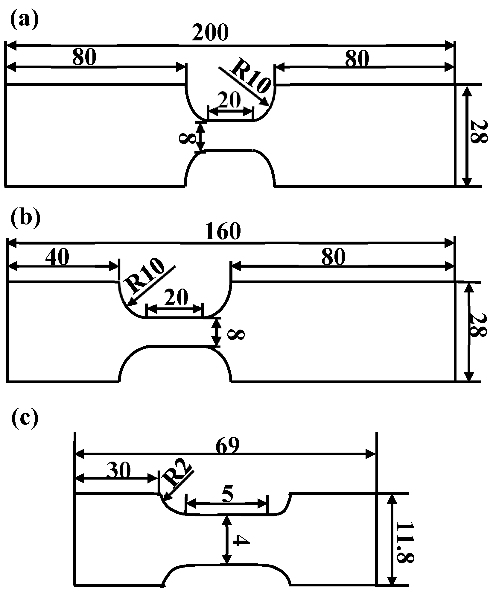
Quasi-static tensile tests were conducted in accordance with GB/T 228.1-2010 standard [28] using a Zwick Z050 (ZwickRoell, HTM 5020, Ulm, Germany) universal testing machine, with strain rates set at 10−3 s−1 and 10−2 s−1. The specimen geometry followed the ISO 26203-2:2011 standard [29], as illustrated in Figure 2a. Dynamic tensile tests were performed on a computer-controlled, electro-hydraulic, servo-driven Zwick-HTM5020 high-speed testing machine, covering strain rates from 10−1 s−1 to 300 s−1, using specimens of identical configuration (Figure 2b).
High-rate tensile testing was carried out on an ARCHIMEDES-ALT1200 split Hopkinson tension bar (SHTB) system (Beijing Orient Dexing Technology Co., Ltd., Beijing, China) [30]. The system employed 18Ni maraging stainless steel for both the incident bar (28 mm diameter × 4800 mm length) and transmission bar (14 mm diameter × 1600 mm length), with a 600 mm long striker bar. The specimen dimensions (Figure 2c) conformed to the GBT 30069.1-2013 standard [31] and were prepared by wire electrical discharge machining. Tests were conducted at strain rates of 1000 s−1, 2000 s−1, and 3000 s−1. To ensure data reliability, triplicate tests were performed for each condition. Engineering stress–strain data were converted to true stress–strain values using standard equations for uniaxial tension. Subsequent analyses was performed on the experimental results.

3. Tensile Test Results and Discussion

3.1. Tensile Mechanical Properties

Figure 3a–c present the true stress–strain curves of 22MnB5 steel at different strain rates. The tensile curves exhibit no distinct yield plateau. Both quasi-static and dynamic tensile tests demonstrate that the material strength increases with rising flow stress. However, upon reaching the yield strength, significantly greater loading is required to induce further plastic deformation, indicative of pronounced strain hardening behavior. As the flow stress continues to increase, the material enters the necking phase until final fracture occurs. While the flow stress–strain profiles show minimal variation across different strain rates, high-rate tensile testing reveals notable phenomena: rapid cross-sectional area reduction at the fracture zone due to sharply increasing flow stress, and the emergence of dynamic softening effects characterized by flow stress decline after attaining ultimate tensile strength, followed by a brief plateau prior to material failure. A marked disparity in stress–strain responses was observed across different strain rates. A. Bardelcik et al. [32] systematically investigated the strain rate sensitivity of martensitic steels through meticulously designed multi-rate tensile tests. Their findings align remarkably with those of the present study, demonstrating negligible variations in mechanical response at strain rates below 103 s−1, while exhibiting pronounced rate-dependent characteristics when the strain rate exceeds 103 s−1 [33]. The figures distinctly reveal pronounced serrated fluctuations in the true stress–strain curves during high-rate tensile testing. Notably, these serrations initiate at a strain rate of 0.1 s−1, albeit with limited amplitude. This phenomenon is currently explained by two primary mechanisms: (1) intrinsic characteristics of the testing apparatus, such as the significant variation in yield strength observed during high-speed tensile testing that may be related to the testing equipment; and (2) the interplay between dynamic strain aging (DSA), strain hardening, and thermal softening effects resulting from the collective motion of solute atoms and dislocations within the material matrix [22,33,34,35]. At lower strain rates, dislocation activation occurs gradually, rendering the DSA effects less prominent while strain hardening dominates. With increasing strain rates, accelerated dislocation multiplication enhances DSA manifestation, leading to marked serrations in high-rate tests. However, the substantial heat generated from rapid projectile impacts during high-velocity testing introduces non-negligible thermal softening effects. The observed attenuation of serration amplitude with increasing strain rates reflects the competitive interaction between DSA and thermal softening mechanisms. Figure 4 presents the temperature-dependent true stress–strain responses of 22MnB5 steel, demonstrating significant thermal influence on mechanical behavior. The pronounced thermal softening effect is clearly evidenced by the progressive stress reduction with elevated temperatures.
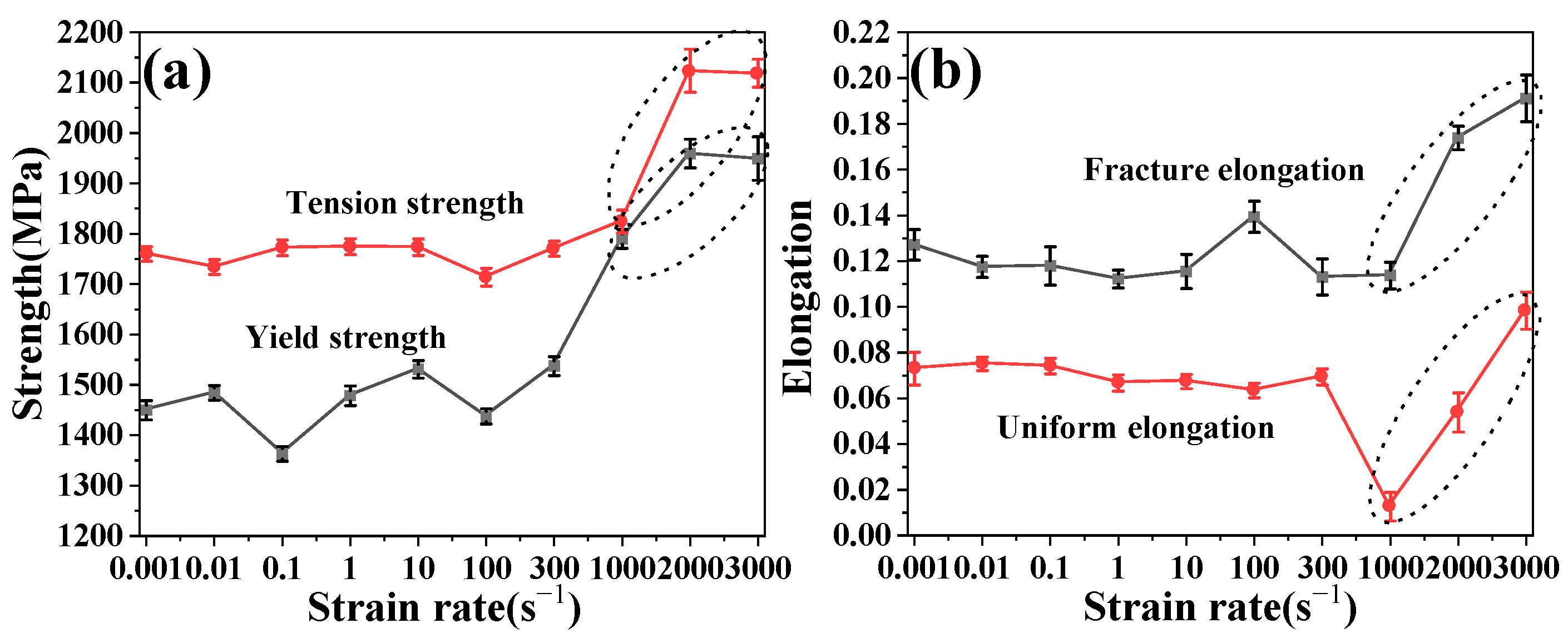
Figure 5 presents the strength and elongation characteristics of 22MnB5 steel under varying strain rate tensile tests. The tensile strength (1577 MPa) of 22MnB5 steel after 900 °C heat treatment with water quenching, as reported by Çavuşoğlu, O. et al. [36], shows slight variation from our results. The uniform elongation, defined as the elongation prior to necking onset (corresponding to ultimate tensile strength), and fracture elongation, representing the elongation at fracture point, are quantitatively analyzed. As evidenced in Figure 5, both yield strength and tensile strength exhibit nonlinear variations with increasing strain rates. Figure 5b further demonstrates that neither fracture elongation nor uniform elongation follows a linear strain rate dependence, maintaining approximately 7% and 12%, respectively. The uniform elongation of the high-speed tensile test material shows linear growth, about 6%, and the fracture elongation is relatively flat. The overall elongation is about 10%. When the strain rate is 100 s−1, the fracture elongation of the material is the highest and the plasticity of the material is better. The material demonstrates overall strain rate insensitivity, consistent with existing lath martensite studies [33,37,38] that identify martensitic steels as rate-insensitive materials. However, under sufficiently high strain rates (indicated by dashed circles), significant strength enhancement is observed. The 22MnB5 steel exhibits characteristic yield strength of ~1500 MPa and tensile strength of ~2000 MPa.

3.2. Sensitivity Coefficient and Strengthening Mechanism

The strain rate sensitivity index at different strain rates is calculated from the stress–strain curve obtained from the test. The strain rate sensitivity m1 of the flow stress can be calculated according to the following equations [39,40]:
m 1 = ln σ t ln ε ˙
where σt is the flow stress and ε ˙ is the strain rate.
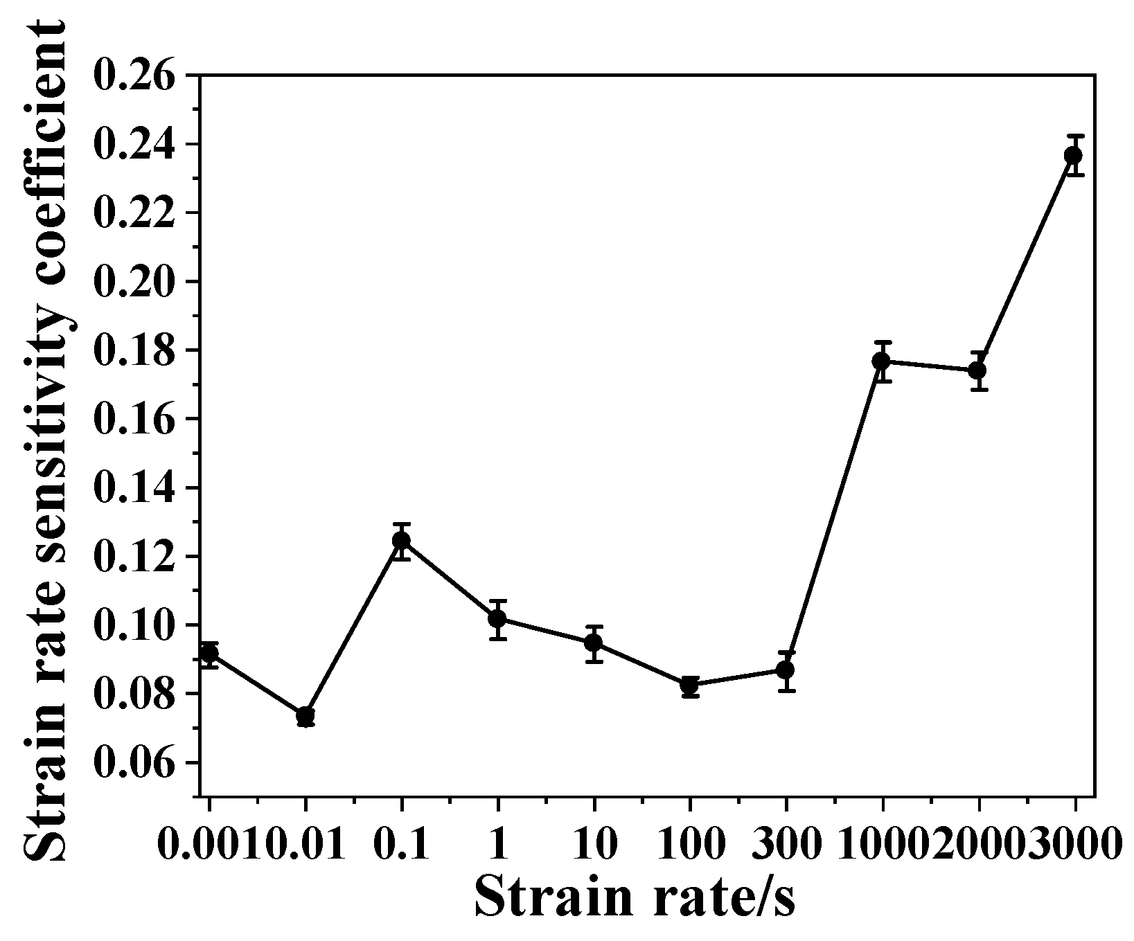
The computational results demonstrate that 22MnB5 steel does not exhibit significant strain rate sensitivity. As shown in Figure 6, the strain rate sensitivity index (m1-value) fails to display a distinct linear correlation with increasing strain rates. Specifically, under relatively low strain rate conditions (at 0.1 s−1), the m1 value undergoes considerable fluctuation. However, subsequent increases in strain rate do not induce substantial variations in m1 values until reaching ultra-high strain rates (1000 s−1), where a dramatic enhancement in m1 value is observed. This phenomenon strongly indicates that material strength characteristics become markedly influenced under extreme high-rate deformation conditions.
The plastic deformation of materials is intrinsically associated with the generation and motion of dislocations within their microstructure. During metallic deformation, multiple microstructural mechanisms including grain boundary rotation, dislocation slip, entanglement, and annihilation collectively mediate the deformation process. As a typical martensitic steel, 22MnB5 possesses an inherently high dislocation density [39,40]. Under quasi-static strain rate conditions, the gradual deformation process facilitates relatively slow dislocation movement, allowing sufficient time for solute atom diffusion. However, only approximately 18% of mobile screw dislocations within the martensitic structure possess adequate activation energy for complete mobilization [41], leading to the formation of shear bands that propagate through the martensitic matrix. The development of these shear bands introduces significant microstructural heterogeneity, generating substantial strain gradients along their boundaries. To accommodate continued deformation while maintaining structural stability, these localized strain concentrations ultimately precipitate ductile fracture through strain localization mechanisms. With increasing strain rates, a marked escalation in screw dislocation liberation occurs within the lath martensite structure, resulting in extensive dislocation pile-up formation and consequent dramatic increases in dislocation density. This phenomenon significantly intensifies strain hardening behavior. During this process, the collapse of lath boundaries occurs, followed by grain refinement within the martensitic laths to achieve structural stability. These microstructural evolutions lead to substantial strength enhancement, becoming particularly pronounced at strain rates reaching 1000 s−1. The concomitant effects include a significant improvement in material strength but a reduction in elongation capacity.

4. Johnson–Cook Constitutive Model

4.1. Establishment of Constitutive Model

Under the conditions of large deformation, high strain rates, and elevated temperatures, the constitutive behavior of metallic materials can be effectively characterized using the Johnson–Cook (J-C) model [21]. As a phenomenological constitutive model, the Johnson–Cook formulation is widely employed to predict the flow stress of materials due to its mathematical simplicity and computational efficiency. The model expresses the flow stress (σ) as follows [42]:
σ = ( A + B ε n ) ( 1 + C ln ε ˙ * ) ( 1 - T * m )
Among them, σ represents the von Mises equivalent stress while ε denotes the equivalent plastic strain. The model incorporates five material parameters: A corresponds to the quasi-static yield strength under reference conditions (typically a room temperature of 20 °C and a strain rate of 10−3 s−1), B represents the strain hardening coefficient, n is the strain hardening exponent, C characterizes the strengthening coefficient of strain rate, and m quantifies the thermal softening behavior. εn, ε ˙ * , and T*m represent the strain hardening effect, strain rate strengthening effect, and temperature effect, respectively, which affect the flow stress value.
In the constitutive formulation, the dimensionless strain rate ( ε ˙ * ) and homologous temperature (T*m) are defined as [43]
ε ˙ * = ε ˙ ε ˙ r e f
T * m = T T r e f T m T r e f
where Tm is the melting temperature of the material, T is the current temperature, εref and Tref are the reference strain rate and the reference temperature. For this study, the reference rate is 0.001 s−1 under quasi-static conditions and the reference temperature is 293 K.
Considering that the high-speed tensile tests were conducted under isothermal room-temperature conditions (T = 293 K), the thermal softening effect becomes negligible. By omitting the temperature-dependent term, the Johnson–Cook constitutive model can be simplified to the following form for quasi-static tensile conditions at ambient temperature as Equation (5):
σ = ( A + B ε n )
Under these conditions, where both strain rate dependence and thermal softening effects are neglected, the Johnson–Cook model reduces to its strain-hardening component. Through algebraic manipulation and logarithmic transformation, the relationship can be linearized as follows:
ln σ A = ln B + n ln ε
A reference strain rate of 0.001 s−1 was established for quasi-static tensile conditions. The corresponding flow stress (σ) and plastic strain (ε) data under these reference conditions were incorporated into the constitutive model to establish the linear relationship between ln(σA) and lnε through logarithmic transformation. Then, the first-order linear regression analysis was performed on the transformed data, with the yield stress A fixed at 1452.03 MPa (corresponding to the stress at zero plastic strain), and the obtained regression curve is shown in Figure 7. The slope of the fitting curve is n value and the intercept is lnB value, so that the material constants B and n are 1201.14 and 0.56, respectively. Based on these determined parameters, the simplified Johnson–Cook constitutive model under quasi-static conditions can be expressed as Equation (7):
σ = 1452.03 + 1201.14 ε 0.56
By maintaining isothermal conditions (T = 293 K) and consequently neglecting thermal softening effects, the strain rate sensitivity parameter C can be determined through the following analytical procedure [44]. The Johnson–Cook model is reformulated to isolate the strain rate dependence:
σ A + B ε n = 1 + C ln ε ˙ *
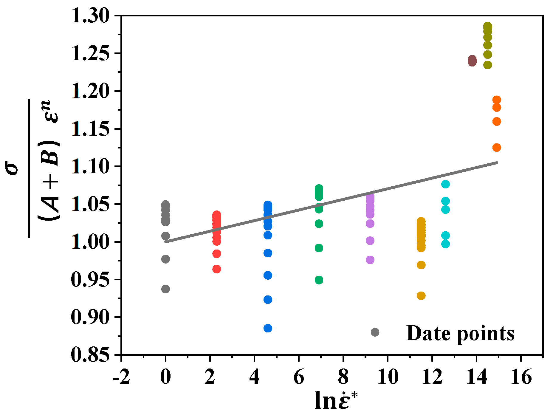
The previously calibrated material parameters (A = 1452.03 MPa, B = 1201.14 MPa, n = 0.56) were systematically incorporated into the Johnson–Cook constitutive relation. Subsequently, the normalized stress term σ / A + B ε n was plotted against the logarithmic strain rate ratio ln ε ˙ * , as illustrated in Figure 8. Subsequently, linear fitting was carried out using the first-order regression model with an intercept value of 1, considering flow stress values at ten strain rates (0.001 s−1, 0.01 s−1, 0.1 s−1, 1 s−1, 10 s−1, 100 s−1, 300 s−1, 1000 s−1, 2000 s−1, 3000 s−1). The slope of the linear fit, representing the strain rate sensitivity coefficient C, was determined to be 0.00704. The complete Johnson–Cook constitutive model was subsequently expressed as Equation (9):
σ = ( 1452.03 + 1201.14 ε 0.56 ) ( 1 + 0.00704 ln ε ˙ * )
The third term in the Johnson–Cook constitutive formulation characterizes the thermal softening behavior of the material, where m represents the temperature sensitivity coefficient. To isolate this thermal effect, the constitutive relation can be transformed as follows:
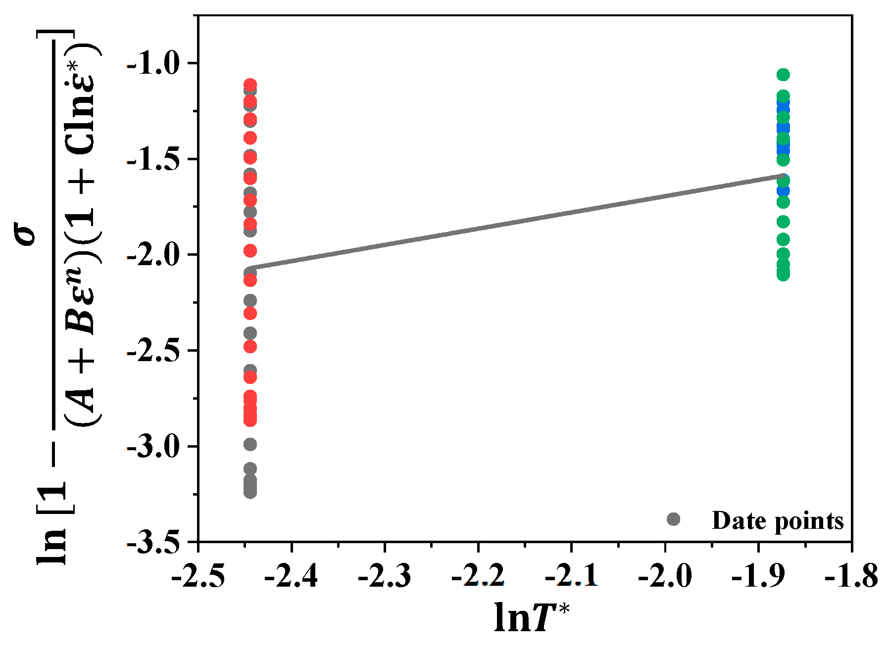
ln 1 σ ( A + B ε n ) ( 1 + C ln ε ˙ * ) = m ln T *
The previously determined material constants (A = 1452.03 MPa, B = 1201.14 MPa, n = 0.56) were systematically incorporated into the constitutive equation. Through algebraic manipulation, the following expression was derived as Equation (11):
ln 1 σ ( 1452.03 + 1201.14 ε 0.56 ) ( 1 + 0.00704 ln ε ˙ * ) = m ln ( T T r e f T m T r e f )
The melting temperature of 22MnB5 steel is 1517.63 °C, that is, Tm = 1517.63 °C, take Tref′ = 20 °C. The first-order regression model is shown in Figure 9, and the m value is obtained as 0.84736.
The complete set of material parameters (A, B, n, C, m) was systematically incorporated into the Johnson–Cook constitutive framework to establish the final flow stress model for 22MnB5 boron steel. As summarized in Table 2, these calibrated parameters comprehensively characterize the material’s thermomechanical response. The full Johnson–Cook formulation is given as Equation (12):
σ = ( 1452.03 + 1201.14 ε 0.56 ) ( 1 + 0.00704 ln ε ˙ * ) ( 1 T * 0.84736 )
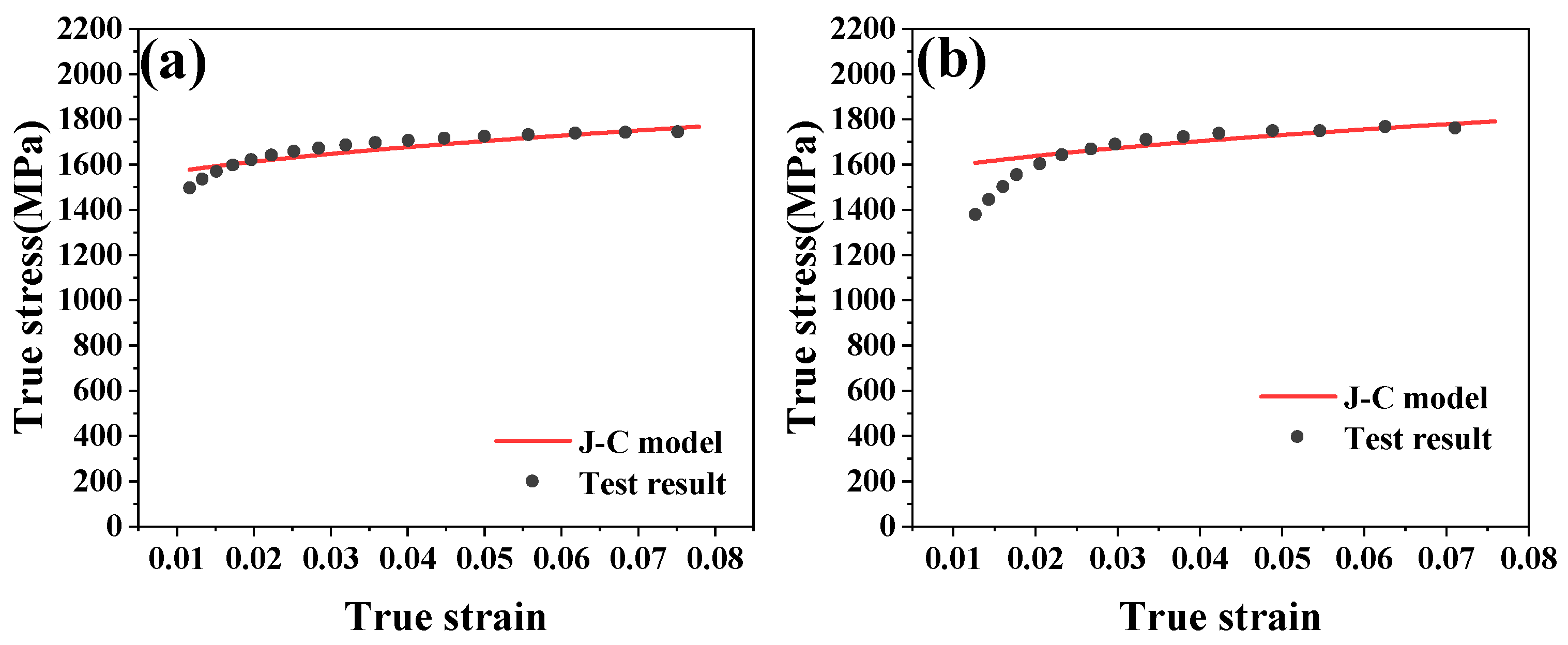
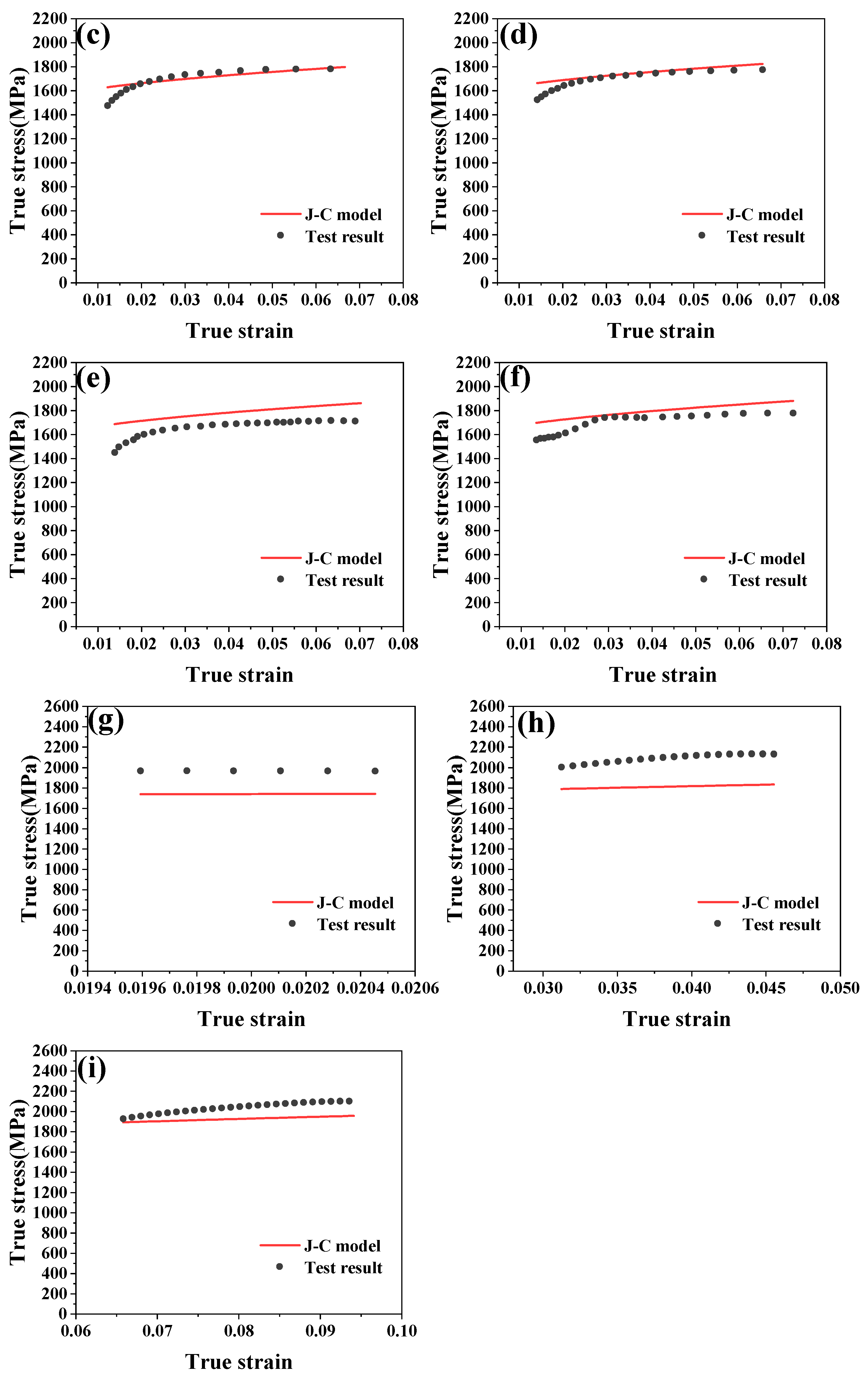
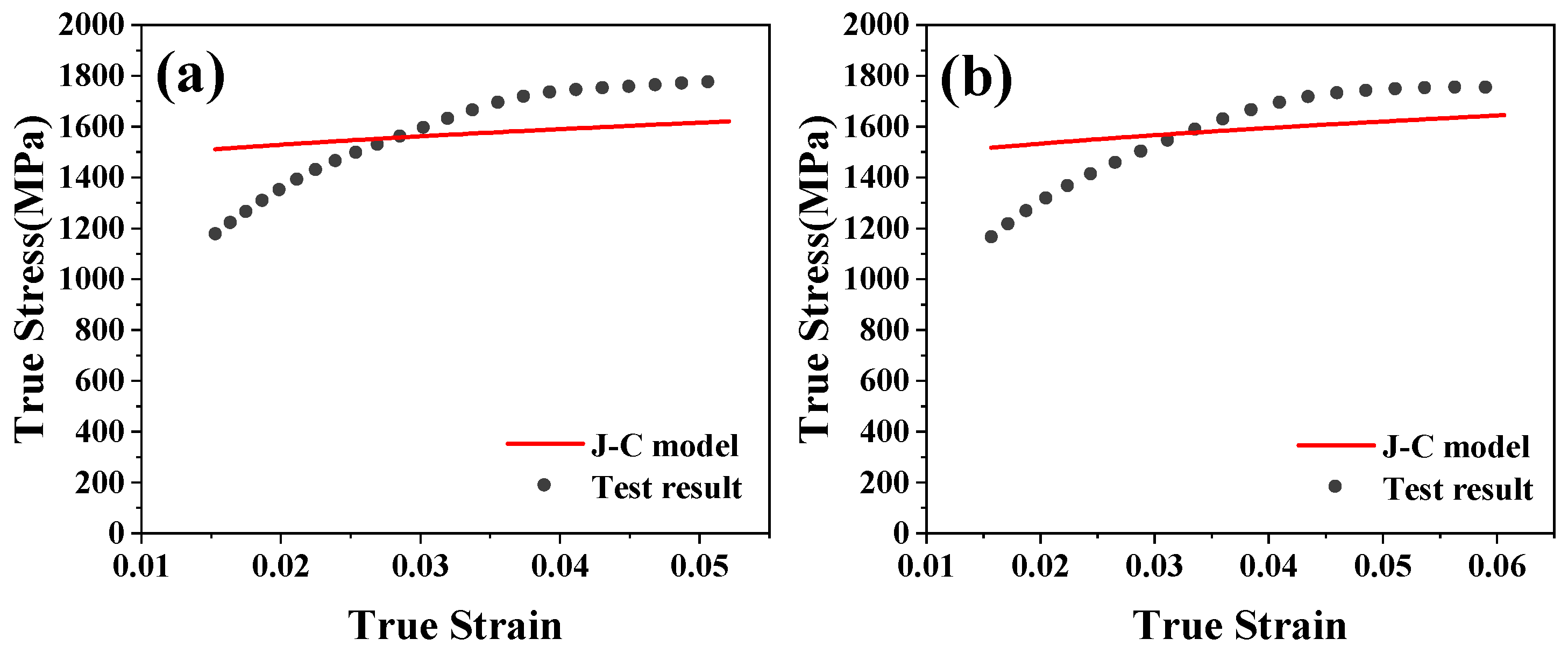
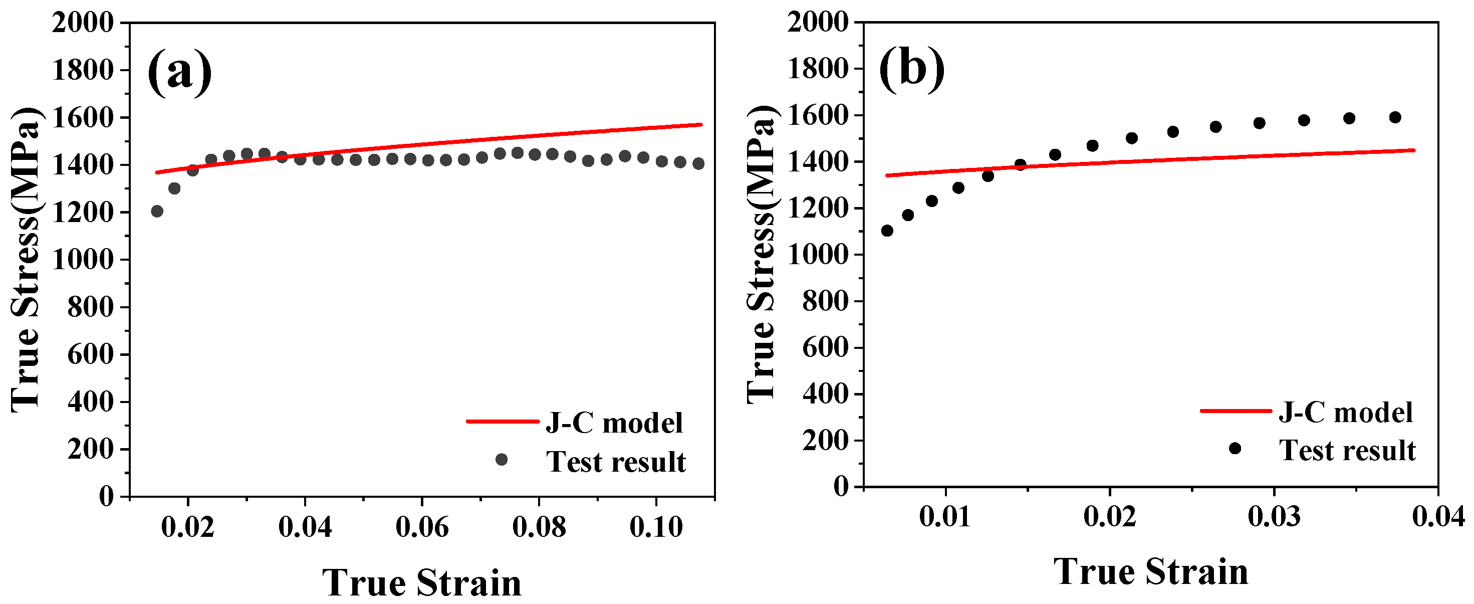
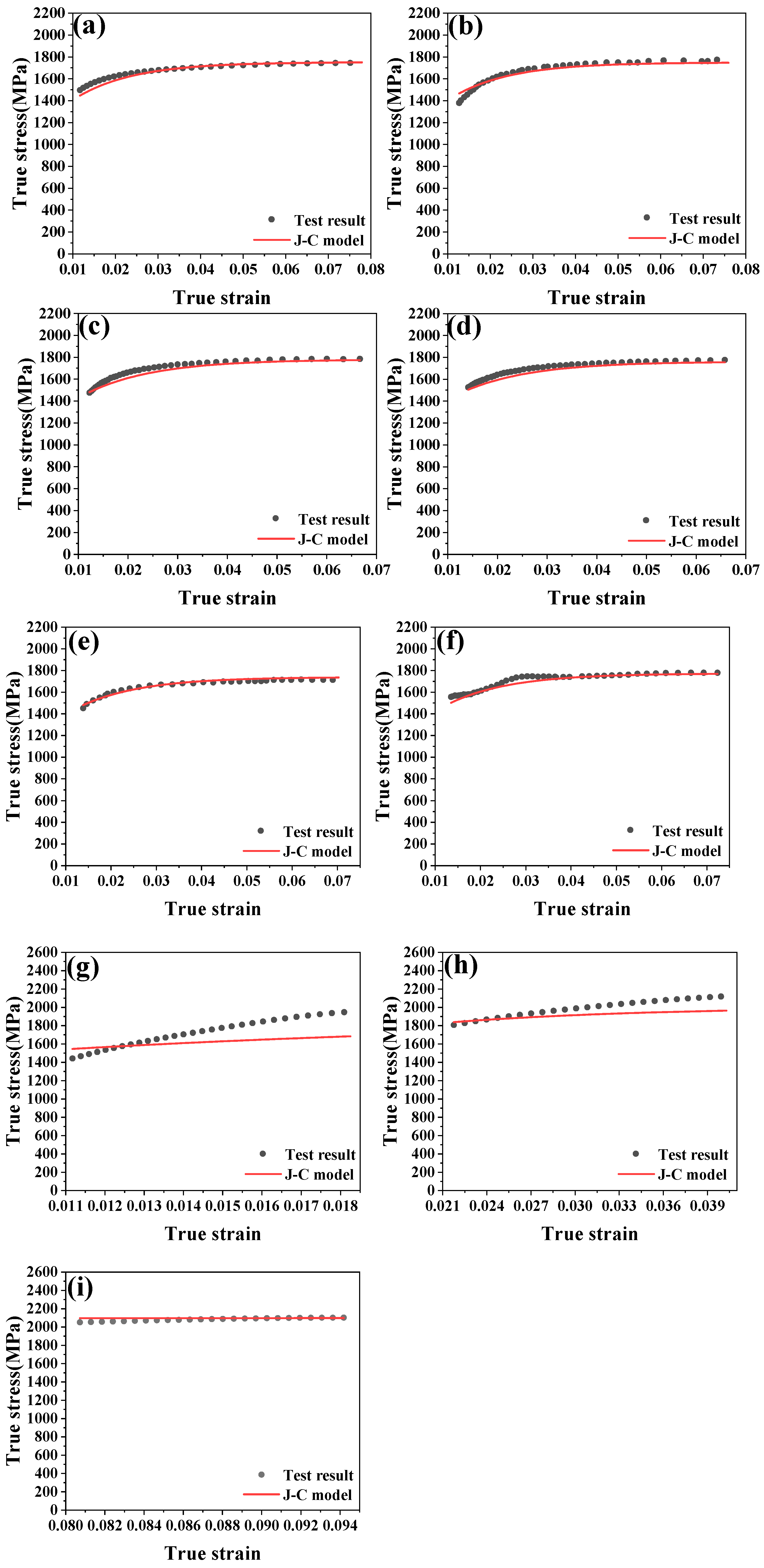
The predictive capability of the obtained Johnson–Cook constitutive model was evaluated by comparing simulated stress–strain curves with experimental data across various strain rates (Figure 10, Figure 11 and Figure 12). The comparative analysis reveals systematic deviations between the model predictions and experimental measurements. These discrepancies indicate that while the standard Johnson–Cook formulation captures the general trend, it requires modification to accurately represent the complex thermomechanical response of 22MnB5 steel.

4.2. Modified Johnson–Cook Constitutive Modeling and Validation

The Johnson–Cook (J-C) constitutive model, while widely adopted for its computational efficiency and parametric simplicity, exhibits fundamental limitations in accurately characterizing the coupled thermomechanical behavior of metallic materials under dynamic loading conditions. The original Johnson–Cook model assumes that thermal softening, strain rate hardening, and strain hardening are three independent phenomena, which are separate from each other [43]. However, in practice, these three have a coupling effect on the flow behavior of steel. From the fitting curve of the original Johnson–Cook equation, it can be clearly seen that the fitting effect of the room-temperature high-speed tensile test (1000 s−1, 2000 s−1, 3000 s−1) is poor. Therefore, in order to describe this effect more accurately, it is necessary to modify the Johnson–Cook model twice [42].
σ = a 1 + a 2 e a 3 ε · f ( ln ε ˙ * ) · 1 c 1 T *
where a 1 + a 2 e a 3 ε represents the relationship between stress and strain strengthening effect [45], and f ( ln ε ˙ * ) represents the influence of strain hardening, that is, the relationship between strain and strain rate.
At reference temperature and reference strain rate (20 °C, 0.001 s−1), the equation was simplified to Equation (14) [46]:
σ = a 1 + a 2 e a 3 ε
The fitting polynomial obtained a 1 = 1771.29045, a 2 = −726.78602, a 3 = −72.78602. When the plastic strain of the material was zero at the reference temperature, the equation was simplified as Equation (15):
σ = a 1 · f ( ln ε ˙ * )
In computational material modeling with limited experimental datasets, the adoption of more sophisticated constitutive equations may enhance the fitting accuracy for specific calibration data. However, this approach inherently establishes a critical trade-off between model complexity and generalization capacity. More specifically, while advanced constitutive formulations can achieve excellent fitting performance within the calibration domain (typically improving the coefficient of determination R2 by 0.15–0.25 and reducing root-mean-square error by 5–8%), their predictive reliability under extrapolated conditions often deteriorates significantly (with extrapolation errors potentially increasing by 30–40%). This overfitting phenomenon, stemming from excessive model parameterization, manifests three major issues: (i) non-physical parameter correlations (|ρ| > 0.9); (ii) heightened sensitivity to experimental noise; and (iii) ill-posed inverse problems in parameter identification (condition number > 103). The fundamental challenge in constitutive modeling under data-limited conditions presents a dualistic optimization problem between model fidelity and generalizability [47]. This critical balance can be formally characterized through several key considerations:
f 1 ( ln ε ˙ * ) = b 11 + b 12 ln ε ˙ * + b 13 ln ε ˙ * 2
f 2 ( ln ε ˙ * ) = b 21 + b 22 ln ε ˙ * + b 23 ln ε ˙ * 2 + b 24 ln ε ˙ * 3
f 3 ( ln ε ˙ * ) = b 31 + b 32 ln ε ˙ * + b 33 ln ε ˙ * 2 + b 34 ln ε ˙ * 3 + b 35 ln ε ˙ * 4
The experimental dataset was systematically partitioned into two distinct subsets to ensure robust model development and validation:
f 1 ( ln ε ˙ * ) = 0.98786 0.0298 ln ε ˙ * + 0.00239 ln ε ˙ * 2
f 2 ( ln ε ˙ * ) = 0.84237 + 0.06035 ln ε ˙ * 0.01072 ln ε ˙ * 2 + 5.30941 e 4 ln ε ˙ * 3
f 3 ( ln ε ˙ * ) = 1.231 0.236 ln ε ˙ * + 0.058 ln ε ˙ * 2 0.0055 ln ε ˙ * 3 + 1.7934 e 4 ln ε ˙ * 4
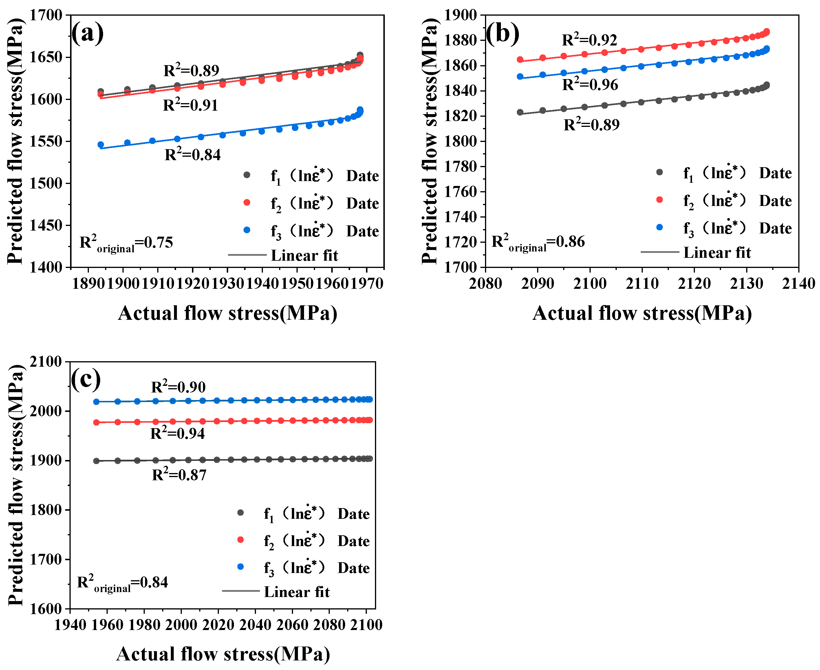
When the strain rate reaches or exceeds 1000 s−1 at room temperature, the predictive capability of the original constitutive model deteriorates significantly. This investigation therefore focuses specifically on model performance under high-strain-rate conditions. To quantitatively evaluate the fitting accuracy between experimental data and the developed constitutive models, the coefficient of determination (R2) is employed as a statistical metric. The R2 value, bounded between 0 and 1, serves as a robust indicator of model fidelity, with values approaching 1 denoting superior fitting performance and higher predictive reliability of the constitutive equation. The mathematical formulation of R2 is expressed as Equation (22) [48,49,50]:
R 2 = ( x x ¯ ) ( y y ¯ ) ( x x ¯ ) 2 ( y y ¯ ) 2 2 = 1 S S _ r e s S S _ t o t = 1 ( y y ^ ) 2 ( y y ¯ ) 2
where SS_res and SS_tot represent the residual and total sum of squares, respectively. This metric provides critical insights into model reliability for high-rate applications while accounting for the complex thermo-mechanical coupling inherent to such extreme loading conditions.
Figure 13 presents a comparative evaluation of the predictive performance for modified constitutive equations of varying complexity levels, as validated against the experimental test dataset.
The comparative analysis presented in Figure 13 demonstrates that the Johnson–Cook model incorporating the f 2 ( ln ε ˙ * ) yields optimal fitting performance, as evidenced by its superior agreement with experimental data across the investigated strain rate regime (R2 = 0.93 ± 0.02). Under isothermal conditions (T = 293 K), where thermal softening effects can be neglected, the simplified Johnson–Cook constitutive relation reduces to the following form as Equation (23):
σ = a 1 + a 2 e a 3 ε · b 21 + b 22 ln ε ˙ * + b 23 ln ε ˙ * 2 + b 24 ln ε ˙ * 3
To quantitatively characterize the temperature-dependent material response, the constitutive formulation is transformed into the following modified expression (Equation (24) [43,45]):
σ a 1 + a 2 e a 3 ε · b 1 + b 2 ln ε ˙ * + b 3 ln ε ˙ * 2 + b 4 ln ε ˙ * 3 = 1 c 1 T *
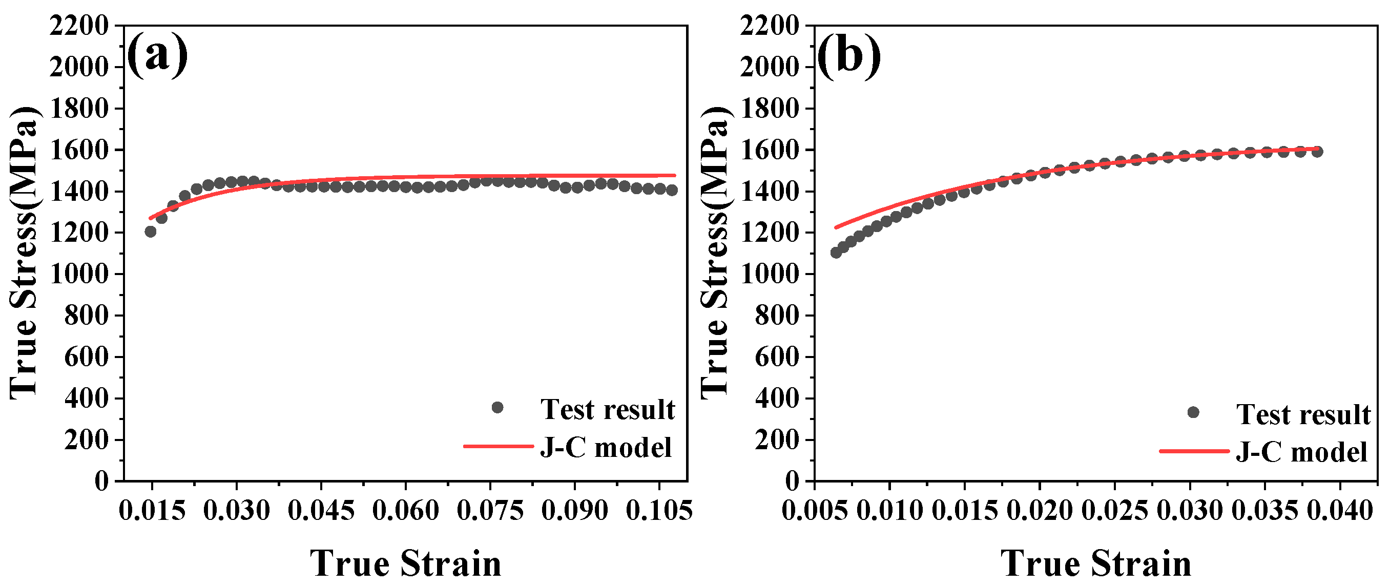
Fitting equation, c1 = 1.523. The predictive capability of the modified Johnson–Cook constitutive model was systematically validated through a comprehensive comparison with experimental stress–strain responses across a wide range of strain rates (0.001–3000 s−1) and temperatures (293, 423 K, 523 K), as illustrated in Figure 14, Figure 15 and Figure 16. The quantitative analysis demonstrates excellent agreement between model predictions and experimental data, with an average coefficient of determination R2 = 0.94 ± 0.03 and maximum relative error below 8% under dynamic loading conditions. The modified formulation significantly improves upon the original model by more accurately capturing three key aspects of 22MnB5 high-strength steel behavior: (1) enhanced strain rate sensitivity, particularly in the high-strain-rate regime ( ε ˙ > 1000 s−1); (2) temperature-dependent work hardening and softening characteristics; and (3) dislocation drag effects at ultra-high deformation rates. These results confirm that the modified Johnson–Cook constitutive relation [42] provides a robust and physically consistent framework for modeling the thermomechanical response of advanced high-strength steels under complex loading conditions.

4.3. Johnson–Cook Damage Model

Johnson and Cook developed a pioneering damage initiation criterion that incorporates three fundamental failure mechanisms through a coupled phenomenological formulation. The Johnson–Cook (J-C) damage model, expressed as Equation (25) [51], has become a benchmark in computational fracture mechanics due to its robust yet computationally efficient framework.
D = Δ ε p ε f
where D is the damage parameter (0 ≦ D < 1), the initial D = 0, when D = 1, the material fails; Δεp is the plastic strain increment in a time step. εf is the equivalent failure strain at the stress state, strain rate and temperature of the current time step. The expression of the failure strain εf is [51,52,53]
ε f = ( D 1 + D 2 exp ( D 3 η ) ) ( 1 + D 4 ln ε ˙ * ) ( 1 + D 5 T * )
where η is the stress triaxiality. It can be calculated using the following equation:
η = σ m σ e p = σ 1 + σ 2 + σ 3 3 × 0.5 × σ 1 2 σ 2 2 + σ 2 2 σ 3 2 + σ 3 2 σ 1 2
where σm is the average stress; σep is the equivalent stress; and D1, D2, D3, D4, and D5 are damage model parameters. During plastic deformation leading to fracture, the material’s load-bearing capacity progressively deteriorates due to damage accumulation. This damage-coupled stress–strain relationship can be formally expressed as [52]
σ D = ( 1 D ) σ e q
In Equation (28), σD is the damage stress state. Furthermore, the stress triaxiality and the equivalent stress can be obtained from undamaged material.
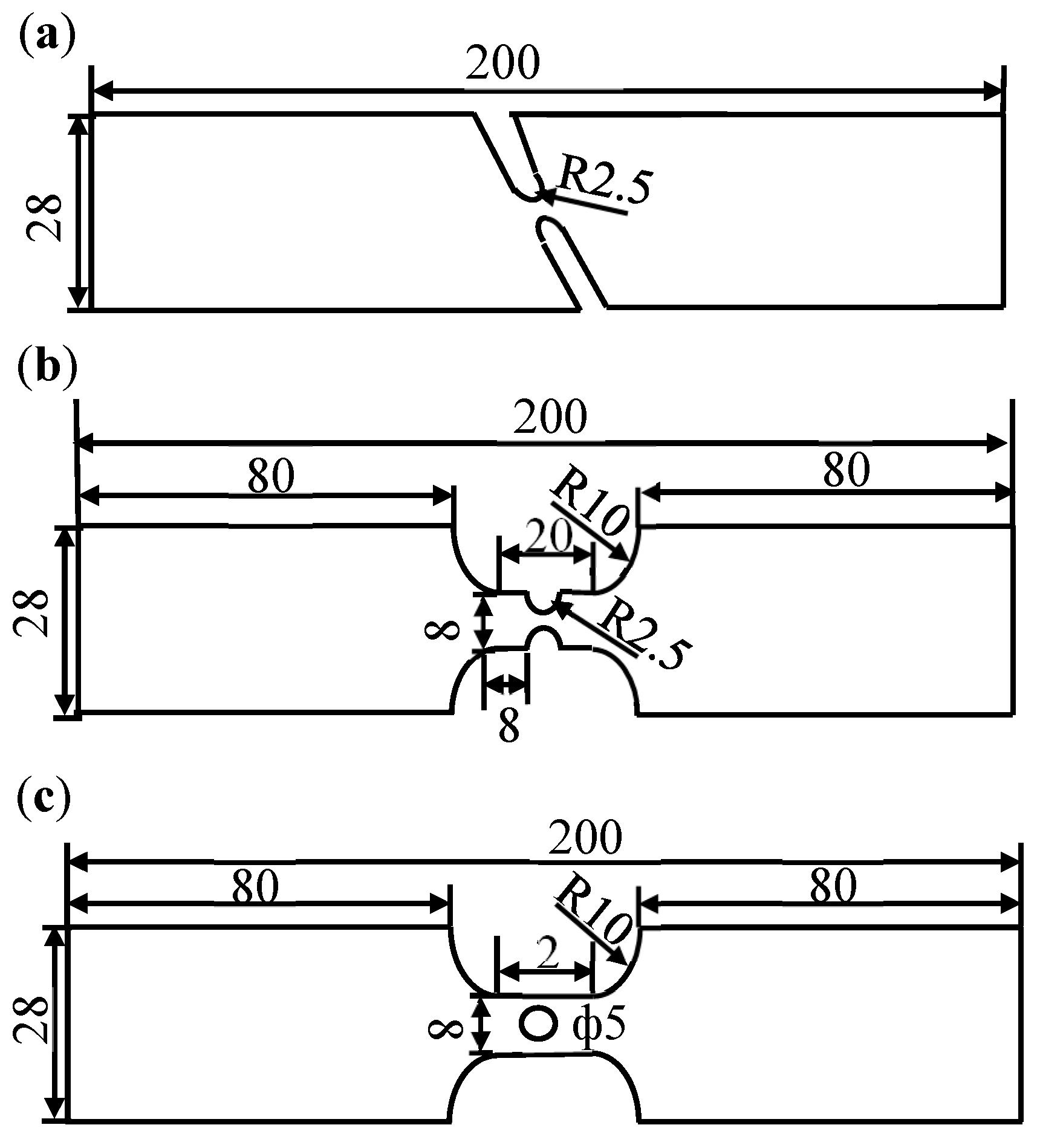
This study systematically investigates the fracture behavior of the test steel under multiaxial stress states by establishing the quantitative relationship between stress triaxiality (η) and fracture strain (εf). Three distinct specimen geometries were precision-machined to achieve controlled stress states: (i) 45° shear specimens for low triaxiality conditions (η ≈ 0), (ii) 2.5 mm radius notched specimens for moderate triaxiality (η ≈ 0.3–0.7), and (iii) 5 mm diameter center-hole specimens for high triaxiality loading (η ≈ 0.5–1.0). The specimen design enables the comprehensive characterization of ductile fracture mechanisms across the entire stress triaxiality spectrum, from shear-dominated to void-growth-dominated failure modes.
The mechanical response of the material was characterized through quasi-static tensile testing ( ε ˙ = 0.001 s−1), with the resulting load–displacement relationship presented in Figure 17. These experimental data were subsequently processed through an integrated computational framework to derive fundamental material properties: (1) the raw load–displacement measurements were converted to true stress–strain curves through finite-element-assisted inverse analysis, accounting for necking effects; and (2) the processed data were systematically partitioned into two distinct regimes [54]—the elastic deformation zone (for modulus determination) and the plastic deformation zone up to necking initiation (for hardening law calibration). This data processing methodology ensures the rigorous characterization of mechanical properties while providing reliable input parameters for subsequent numerical simulations.
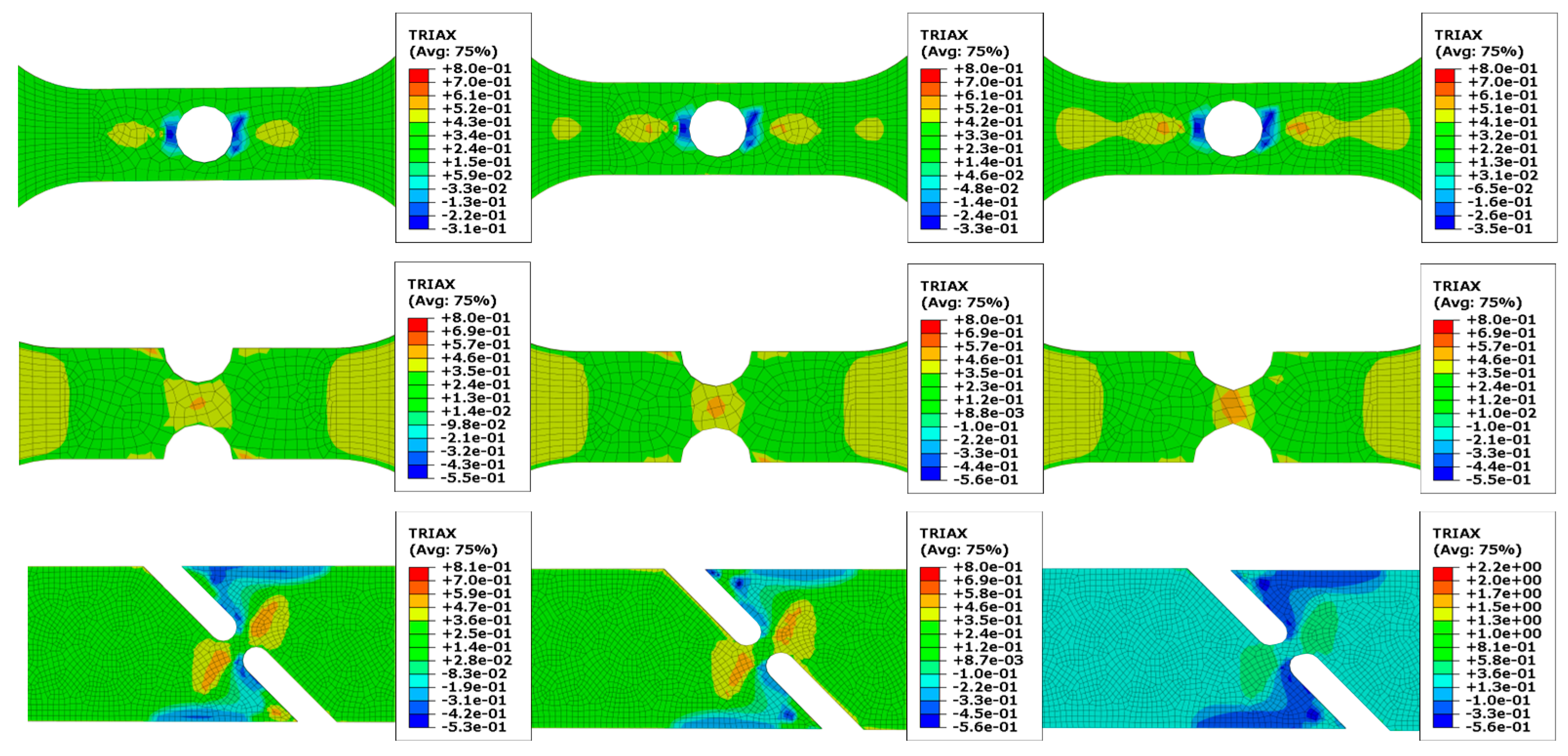
The quantitative fracture characteristics of the test steel, including critical fracture strains and corresponding stress states, are systematically summarized in Table 3. Complementing these experimental results, Figure 18 presents a detailed finite element analysis of the stress triaxiality evolution, specifically including (1) the onset of the plastic stage, (2) tensile deformation through the elastic stage, and (3) the final tensile termination leading to fracture initiation. This combined experimental–numerical approach provides comprehensive insight into the relationship between multiaxial stress states and ductile fracture behavior in the investigated steel alloy.
Under isothermal quasi-static loading conditions ( ε ˙ = 0.001 s−1, T = 293 K), the Johnson–Cook fracture model reduces to the following simplified form (Equation (29) [44]):
ε f = D 1 + D 2 exp ( D 3 η )
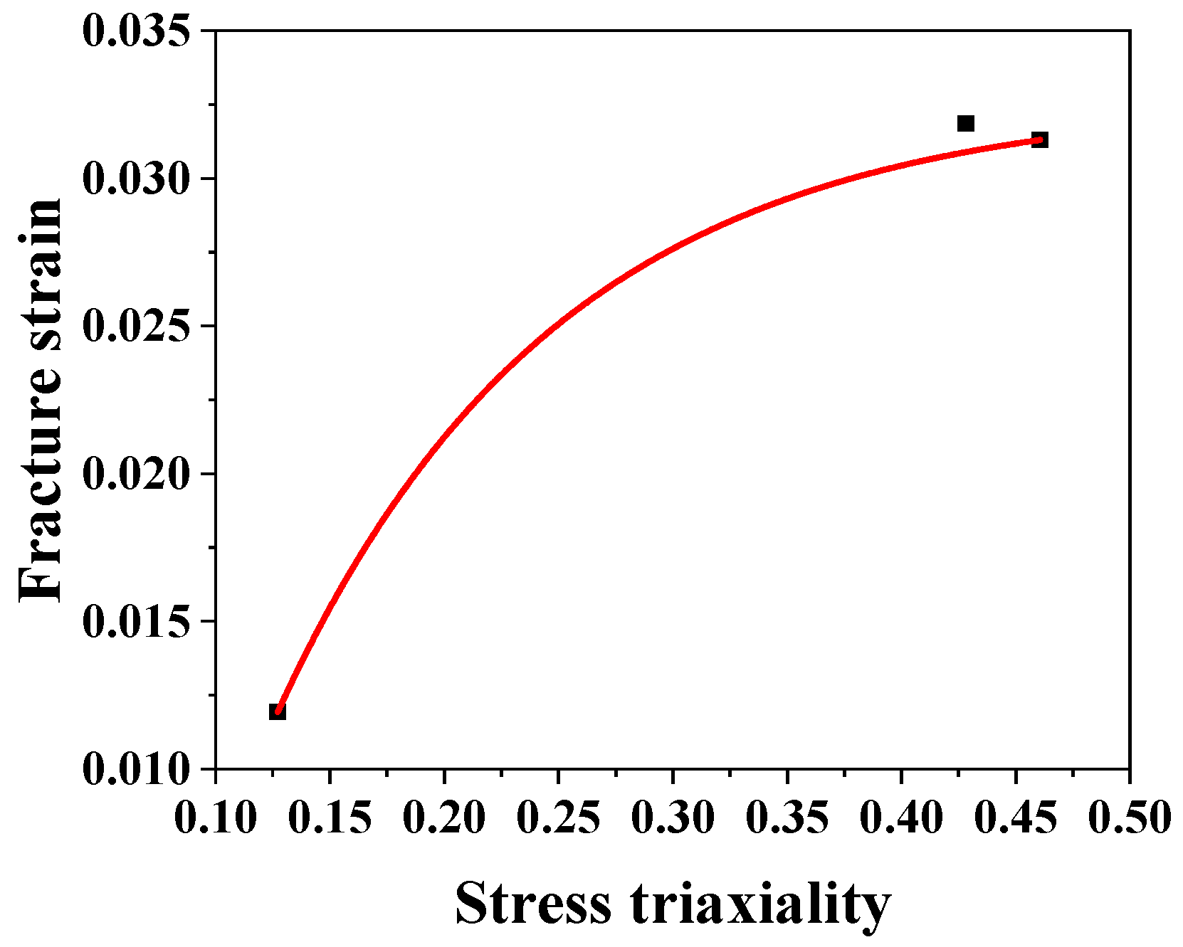
The quantitative relationship between fracture strain (εf) and stress triaxiality (η) was established through the nonlinear regression analysis of the experimental data, as graphically presented in Figure 19. The Johnson–Cook failure model parameters were determined via curve fitting, yielding the following optimized coefficients: D1 = 0.03265 (characterizing the shear-dominated fracture limit), D2 = −0.05868 (governing ductility reduction rate), and D3 = 8.1825 (controlling triaxiality sensitivity).
The parameter D4 represents the strain rate sensitivity coefficient in the Johnson–Cook (J-C) ductile fracture model, characterizing the influence of deformation rate on material failure. Having previously established the stress-state-dependent parameters (D1, D2, D3) through comprehensive calibration under varying triaxiality conditions, the current study focuses on determining D4 through isothermal testing (T = 293 K ± 2 K). By maintaining constant stress triaxiality (η = D, where D is a predetermined reference value), the fracture strain becomes exclusively dependent on strain rate effects, enabling the J-C failure criterion to be reduced to the following simplified form (Equation (30)):
ε f = D ( 1 + ε ˙ * ) D 4
By applying logarithmic transformation to both sides of Equation (30), we derive the linearized form for parameter identification:
ln ε f = ln D + D 4 ln ( 1 + ε ˙ * )
By fitting the relationship curve between the logarithm of fracture strain and the logarithm of strain rate, D4 = −2.82663 can be obtained.
D5 is the temperature constant of the J-C failure model, so the J-C failure model of 22MnB5 steel at different strain rates without considering the temperature can be expressed as Equation (32):
ε f = ( 0.03265 + 0.05868 exp ( 8.1825 η ) ) ( 1 2.826631 ln ε ˙ * )

5. Conclusions

(1) The tensile mechanical properties of 22MnB5 high-strength steel were measured by tensile experiments at different strain rates. The results show that the overall yield strength and tensile strength of 22MnB5 steel are about 1500 MPa, and the uniform elongation and fracture elongation are maintained at about 7% and 12%, respectively, in the tensile test of 10−3 s−1~300 s−1 at room temperature (20 °C). When the strain rate reaches 1000 s−1~3000 s−1, the yield strength and tensile strength of the material are about 2000 MPa, while the uniform elongation and fracture elongation are maintained at about 6% and 10%, respectively.
(2) 22MnB5 steel exhibits strain rate insensitivity, as evidenced by the nonlinear relationship between the strain rate sensitivity factor (m1) and increasing strain rates. At relatively low strain rates, the immobile dislocations within the martensitic laths remain inactivated, leading to the formation of shear bands. This results in strain localization and subsequent ductile fracture. Under high strain rate conditions, the mobilization of previously immobile dislocations occurs, accompanied by the collapse of lath boundaries and the development of extensive dislocation pile-ups. To achieve a stabilized microstructure, grain refinement is induced through dynamic recrystallization mechanisms, consequently enhancing the material’s strength.
(3) Based on the experimental data, the Johnson–Cook constitutive model was established and modified. The coefficient of determination of the modified constitutive model is greater than that of the original constitutive model (R2 = 0.93 ± 0.02), indicating that the modified constitutive model has a better fitting effect on the experimental data.
(4) Combining the finite element and experimental results, the Johnson–Cook failure model was established. The estimated damage model parameters can be used to model metal forming simulations and obtain valuable prediction results for working materials.

Author Contributions

Conceptualization, Y.X. and Y.S.; methodology, Y.X. and Y.S.; investigation, Y.X. and Y.S.; validation, Y.S.; formal analysis, Y.X., Y.S. and G.Y.; resources, Y.X.; writing—original draft preparation, Y.S.; writing—review and editing, Y.X. and Y.S.; visualization, Y.X. and Y.S.; software, Y.S.; supervision, Y.X.; project administration, G.Y.; funding acquisition, Y.X. All authors have read and agreed to the published version of the manuscript.

Funding

This work was supported by the National Key Research and Development Program of China (No. 2021YFB3702402), the National Natural Science Foundation of China (52293393), and the Natural Science Foundation project of Hubei Province (Grant No. 2023AFA062).

Data Availability Statement

The original contributions presented in this study are included in the article. Further inquiries can be directed to the corresponding author.

Acknowledgments

The Analytical & Testing Center of Wuhan University of Science and Technology.

Conflicts of Interest

The authors declare no conflicts of interest.

References

  1. Zhao, H.; Zhang, R.; Bin, Z. A Review of Automotive Lightweight Technology. In Proceedings of the 2018 International Conference on Mechanical, Electronic, Control and Automation Engineering (MECAE 2018), Qingdao, China, 30–31 March 2018; Atlantis Press: Dordrecht, The Netherlands, 2018. [Google Scholar]
  2. Li, Y.; Lin, Z.; Jiang, A.; Chen, G. Use of High Strength Steel Sheet for Lightweight and Crashworthy Car Body. Mater. Des. 2003, 24, 177–182. [Google Scholar] [CrossRef]
  3. Zhang, Z.; Chen, S.; Hong, Y.; Li, X.; Zhang, J.; Xiao, Y.; Luo, G.; Yu, Y.; Hu, J. Multi-Scale Damage Mechanism of Hierarchically Structured High-Strength Martensitic Steels under Shock Loading. Int. J. Plast. 2024, 175, 103945. [Google Scholar] [CrossRef]
  4. Liu, Y.; Li, G.; Wan, X.; Zhang, X.; Shen, Y.; Wu, K. Toughness Improvement by Zr Addition in the Simulated Coarse-Grained Heat-Affected Zone of High-Strength Low-Alloy Steels. Ironmak. Steelmak. 2019, 46, 113–123. [Google Scholar] [CrossRef]
  5. Kumar, A.; Paul, S.K. Local Strain Evolution and Microstructural Characterisation of Hydrogen-Induced Damage at Different Strain Rates in Dual Phase (DP 780) Steel. Forces Mech. 2023, 13, 100237. [Google Scholar] [CrossRef]
  6. Li, Y.; Wang, E.; Zhang, L.; Ma, B.; Du, J.; Zhang, S. High Strength and High Ductility of 60Si2CrVAT Spring Steel through a Novel Quenching and Partitioning (Q-P) Process. Mater. Sci. Eng. A 2024, 899, 146444. [Google Scholar] [CrossRef]
  7. Li, D.-F.; Cheng, J.-H.; Bai, C.-G.; Zhang, Z.-Q.; Du, F.-F.; Wang, R.; Zhao, J.; Li, N.; Yang, R. Multi-Scale α-Phase Heterostructure Induced Transformation-Induced Plasticity (TRIP) Effect in Metastable A+β Titanium Alloy Showing Excellent Strength and Work-Hardening Combination. J. Mater. Process. Technol. 2025, 341, 118880. [Google Scholar] [CrossRef]
  8. Li, B.; Zhu, H.; Sun, J.; Song, M.; Zhao, J. Effect of Ti Addition on Non-Metallic Inclusion Characteristics in TRIP Steel. Steel Res. Int. 2022, 93, 2200064. [Google Scholar] [CrossRef]
  9. Braga, D.P.; Palhares, I.C.; Moreira Afonso, C.R.; Camilo Magalhães, D.C.; Della Rovere, C.A.; Kliauga, A.M. Effects of Temperature, Strain Rate and Grain Size on the Twin Induced Plasticity (TWIP) Effect of an AISI 316 LV Austenitic Stainless Steel. Mater. Sci. Eng. A 2025, 931, 148234. [Google Scholar] [CrossRef]
  10. Zheng, Y.; Zhang, L.; Lin, Y.; Wang, J.; Wang, K.; Guo, Z.; Cao, R.; Zhu, L.; Wang, B.; Zhang, D.; et al. Effect of Compound Addition of Ti–B on Hardenability and Hot Ductility of 22MnB5 Hot Stamped Steel. J. Mater. Res. Technol. 2025, 36, 1173–1193. [Google Scholar] [CrossRef]
  11. Kubota, K.; Ohba, T.; Morito, S. Frictional Properties of New Developed Cold Work Tool Steel for High Tensile Strength Steel Forming Die. Wear 2011, 271, 2884–2889. [Google Scholar] [CrossRef]
  12. Xu, Y.; Ji, Q.; Yang, G.; Bao, S.; Zhao, G.; Miao, X.; Mao, X. Effect of Cooling Path on Microstructures and Hardness of Hot-Stamped Steel. Metals 2020, 10, 1692. [Google Scholar] [CrossRef]
  13. Jiang, C.; Shan, Z.; Zhuang, B.; Zhang, M.; Xu, Y. Hot Stamping Die Design for Vehicle Door Beams Using Ultra-High Strength Steel. Int. J. Precis. Eng. Manuf. 2012, 13, 1101–1106. [Google Scholar] [CrossRef]
  14. Karbasian, H. A Review on Hot Stamping. J. Mater. Process. Technol. 2010, 210, 2103–2118. [Google Scholar] [CrossRef]
  15. Merklein, M.; Wieland, M.; Lechner, M.; Bruschi, S.; Ghiotti, A. Hot Stamping of Boron Steel Sheets with Tailored Properties: A Review. J. Mater. Process. Technol. 2016, 228, 11–24. [Google Scholar] [CrossRef]
  16. Mori, K. Hot Stamping of Ultra-High Strength Steel Parts. CIRP Ann. 2017, 66, 755–777. [Google Scholar] [CrossRef]
  17. Liu, C.; Xiong, F.; Wang, Y.; Cao, Y.; Liu, X.; Xue, Z.; Peng, Q.; Peng, L. Strengthening Mechanism and Carbide Precipitation Behavior of Nb-Mo Microalloy Medium Mn Steel. Materials 2021, 14, 7461. [Google Scholar] [CrossRef] [PubMed]
  18. Liu, Y.; Li, G.; Wan, X.; Wang, H.; Wu, K.; Misra, R.D.K. The Role of Cu and Al Addition on the Microstructure and Fracture Characteristics in the Simulated Coarse-Grained Heat-Affected Zone of High-Strength Low-Alloy Steels with Superior Toughness. Mater. Sci. Technol. 2017, 33, 1750–1764. [Google Scholar] [CrossRef]
  19. Mao, X.; Huo, X.; Sun, X.; Chai, Y. Strengthening Mechanisms of a New 700MPa Hot Rolled Ti-Microalloyed Steel Produced by Compact Strip Production. J. Mater. Process. Technol. 2010, 210, 1660–1666. [Google Scholar] [CrossRef]
  20. Zener, C.; Hollomon, J.H. Effect of Strain Rate upon Plastic Flow of Steel. J. Appl. Phys. 1944, 15, 22–32. [Google Scholar] [CrossRef]
  21. Johnson, G.R.; Cook, W.H. A Constitutive Model and Data for Metals Subjected to Large Strains, High Strain Rates and High Temperatures. In Proceedings of the 7th International Symposium on Ballistics, The Hague, The Netherlands, 19–21 April 1983; pp. 541–548. [Google Scholar]
  22. Roters, F.; Eisenlohr, P.; Hantcherli, L.; Tjahjanto, D.D.; Bieler, T.R.; Raabe, D. Overview of Constitutive Laws, Kinematics, Homogenization and Multiscale Methods in Crystal Plasticity FInite-Element Modeling: Theory, Experiments, Applications. Acta Mater. 2010, 58, 1152–1211. [Google Scholar] [CrossRef]
  23. Zerilli, F.J. Dislocation Mechanics-Based Constitutive Equations. Metall. Mater. Trans. A 2004, 35, 2547–2555. [Google Scholar] [CrossRef]
  24. Rusinek, A.; Klepaczko, J.R. Shear Testing of a Sheet Steel at Wide Range of Strain Rates and a Constitutive Relation with Strain-Rate and Temperature Dependence of the Flow Stress. Int. J. Plast. 2001, 17, 87–115. [Google Scholar] [CrossRef]
  25. Steinberg, D.S. Vibration Analysis for Electronic Equipment; Wiley: Hoboken, NJ, USA, 2000; ISBN 978-0-471-37685-9. [Google Scholar]
  26. Non-Linear Analysis of Composite Structure Subjected to Impact Load Based on Johnson-Cook Constitutive Model. Int. J. Non-Linear Mech. 2025, 178, 105176. [CrossRef]
  27. Research on the Expansion and Failure of Solid Expandable Tubular Based on the Johnson-Cook Failure Model. Int. J. Press. Vessel. Pip. 2025, 218, 105567. [CrossRef]
  28. GB/T 228.1-2010; Metallic Materials Tensile Testing-Part 1: Method of Test at Room Temperature. China Standard Publishing House: Beijing, China, 2011.
  29. ISO 26203-2:2011; Metallic Materials—Tensile Testing at High Strain Rates—Part 2: Servo-Hydraulic and Other Test Systems. German Version DIN EN ISO 26203-2:2011. International Organization for Standardization: Geneva, Switzerland, 2011.
  30. Liu, X.; He, Z.; Ye, J.; Yan, L.; Li, S.; Tang, Y. Study on Dynamic Mechanical Behavior of Q460JSC and HQ600 High Strength Steel. J. Constr. Steel Res. 2020, 173, 106232. [Google Scholar] [CrossRef]
  31. GB/T 30069–2013; Metallic Material Tensile Testing at High Strain Rates-Part 1: Elastic Rod Type System. China Standard Publishing House: Beijing, China, 2013.
  32. Bardelcik, A. A Strain Rate Sensitive Constitutive Model for Quenched Boron Steel with Tailored Properties. Int. J. Impact Eng. 2012, 50, 49–62. [Google Scholar] [CrossRef]
  33. Zhang, Z.; Shen, F.; Liu, H.; Könemann, M.; Münstermann, S. Temperature-Dependent Deformation and Fracture Properties of Low-Carbon Martensitic Steel in Different Stress States. J. Mater. Res. Technol. 2023, 25, 1931–1943. [Google Scholar] [CrossRef]
  34. Woo, W.; Em, V.T. Stress–Strain Relationship between Ferrite and Martensite in a Dual-Phase Steel Studied by in Situ Neutron Diffraction and Crystal Plasticity Theories. Acta Mater. 2012, 60, 6972–6981. [Google Scholar] [CrossRef]
  35. Hu, C.; Huang, C.P.; Liu, Y.X.; Perlade, A.; Zhu, K.Y.; Huang, M.X. The Dual Role of TRIP Effect on Ductility and Toughness of a Medium Mn Steel. Acta Mater. 2023, 245, 118629. [Google Scholar] [CrossRef]
  36. Çavuşoğlu, O.; Çavuşoğlu, O.; Yılmazoğlu, A.G.; Üzel, U.; Aydın, H.; Güral, A. Microstructural Features and Mechanical Properties of 22MnB5 Hot Stamping Steel in Different Heat Treatment Conditions. J. Mater. Res. Technol. 2020, 9, 10901–10908. [Google Scholar] [CrossRef]
  37. Guan, J.; Yuan, Q.; Zhang, Q.; Qiao, W.; Xu, G. Simultaneous Enhancement of Strength and Toughness in a Medium-Carbon Martensitic Steel by Ti-Mo Addition. J. Mater. Eng. Perform. 2022, 31, 4273–4281. [Google Scholar] [CrossRef]
  38. Li, C.; Li, X.; Yu, W.; Shi, J.; Wang, M.; Wu, R. Microstructure Characteristics and Strengthening Mechanism of Martensitic Steel at Two Quenching Rates. J. Mater. Eng. Perform. 2022, 31, 8711–8720. [Google Scholar] [CrossRef]
  39. Zhang, Z.; Shen, F.; Münstermann, S. Crystal Plasticity Modeling of Prior Austenite Orientation Effects on Deformation Behaviors of Martensitic Steels under Different Strain Paths. Mater. Des. 2024, 245, 113280. [Google Scholar] [CrossRef]
  40. Krauss, G. Martensite in Steel: Strength and Structure. Mater. Sci. Eng. A 1999, 273–275, 40–57. [Google Scholar] [CrossRef]
  41. Dannoshita, H.; Hasegawa, H.; Matsuda, H.; Gong, W.; Kawasaki, T.; Harjo, S.; Umezawa, O. Evolution of Dislocation Structure Determined by Neutron Diffraction Line Profile Analysis during Tensile Deformation in Quenched and Tempered Martensitic Steels. Mater. Sci. Eng. A 2022, 854, 143795. [Google Scholar] [CrossRef]
  42. Li, N.; Xu, Y.; Yang, G.; Fu, Z. Dynamic Mechanical Properties and Constitutive Model Establishment of QSTE420 Steel. J. Constr. Steel Res. 2024, 213, 108342. [Google Scholar] [CrossRef]
  43. Lin, Y.C.; Chen, X.-M.; Liu, G. A Modified Johnson–Cook Model for Tensile Behaviors of Typical High-Strength Alloy Steel. Mater. Sci. Eng. A 2010, 527, 6980–6986. [Google Scholar] [CrossRef]
  44. Murugesan, M.; Jung, D. Johnson Cook Material and Failure Model Parameters Estimation of AISI-1045 Medium Carbon Steel for Metal Forming Applications. Materials 2019, 12, 609. [Google Scholar] [CrossRef] [PubMed]
  45. Bian, Y. Mechanical Properties and JC Constitutive Modification of Tungsten Alloys under High Strain Rates and High/Low Temperatures. Mater. Today Commun. 2024, 41, 110542. [Google Scholar] [CrossRef]
  46. He, J.; Chen, F.; Wang, B.; Zhu, L.B. A Modified Johnson-Cook Model for 10%Cr Steel at Elevated Temperatures and a Wide Range of Strain Rates. Mater. Sci. Eng. A 2018, 715, 1–9. [Google Scholar] [CrossRef]
  47. Liu, Y. Unbiased Estimate of Generalization Error and Model Selection in Neural Network. Neural Netw. 1995, 8, 215–219. [Google Scholar] [CrossRef]
  48. Murugesan, M.; Kang, B.-S.; Lee, K. Multi-Objective Design Optimization of Composite Stiffened Panel Using Response Surface Methodology. Compos. Res. 2015, 28, 297–310. [Google Scholar] [CrossRef]
  49. Lee, K.; Murugesan, M.; Lee, S.-M.; Kang, B.-S. A Comparative Study on Arrhenius-Type Constitutive Models with Regression Methods. Trans. Mater. Process. 2017, 26, 18–27. [Google Scholar] [CrossRef]
  50. Di Bucchianico, A. Coefficient of Determination (R2). In Encyclopedia of Statistics in Quality and Reliability; John Wiley & Sons, Ltd.: Hoboken, NJ, USA, 2008; ISBN 978-0-470-06157-2. [Google Scholar]
  51. Murugesan, M.; Lee, S.; Kim, D.; Kang, Y.-H.; Kim, N. A Comparative Study of Ductile Damage Models Approaches for Joint Strength Prediction in Hot Shear Joining Process. Procedia Eng. 2017, 207, 1689–1694. [Google Scholar] [CrossRef]
  52. Banerjee, A.; Dhar, S.; Acharyya, S.; Datta, D.; Nayak, N. Determination of Johnson Cook Material and Failure Model Constants and Numerical Modelling of Charpy Impact Test of Armour Steel. Mater. Sci. Eng. A 2015, 640, 200–209. [Google Scholar] [CrossRef]
  53. Buzyurkin, A.E.; Gladky, I.L.; Kraus, E.I. Determination and Verification of Johnson–Cook Model Parameters at High-Speed Deformation of Titanium Alloys. Aerosp. Sci. Technol. 2015, 45, 121–127. [Google Scholar] [CrossRef]
  54. Owen, D.R.J.; Hinton, E. Finite Elements in Plasticity: Theory and Practice; Pineridge Press: Swansea, UK, 1980; ISBN 978-0-906674-05-5. [Google Scholar]
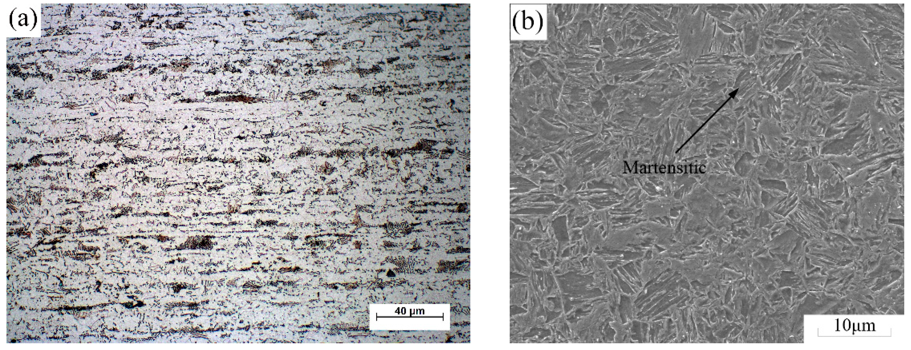
Figure 1. Microstructural morphology of 22MnB5 steel. (a) Optical microscope (as-received); (b) scanning electron microscope (post-quenching).
Metals 15 00811 g001
Figure 2. Size of tensile specimen (unit: mm): (a) static tensile specimen; (b) dynamic tensile specimen; (c) high-speed tensile specimen.
Metals 15 00811 g002
Figure 3. True stress–strain curves of 22MnB5 steel with different strain rates at room temperature (20 °C): (a) 0.001 s−1, 0.01 s−1, 0.1 s−1, 1 s−1; (b) 10 s−1, 100 s−1, 300 s−1; (c) 1000 s−1, 2000 s−1, 3000 s−1.
Metals 15 00811 g003
Figure 4. True stress–strain curves of 22MnB5 steel at different temperatures: (a) 1000 s−1; (b) 2000 s−1; (c) 3000 s−1.
Metals 15 00811 g004
Figure 5. Variations in true stress and elongations with increasing strain rate: (a) yield strength and ultimate tensile strength; (b) uniform elongation and fracture elongation.
Metals 15 00811 g005
Figure 6. Strain rate sensitivity coefficients with different strain rates.
Metals 15 00811 g006
Figure 7. Relationship between ln(σA) and lnε under the reference conditions.
Metals 15 00811 g007
Figure 8. Relationship between σ / A + B ε n and ln ε ˙ * under the reference conditions.
Metals 15 00811 g008
Figure 9. Relationship between ln 1 σ ( A + B ε n ) ( 1 + C ln ε ˙ * ) and lnT* under the reference conditions.
Metals 15 00811 g009
Figure 10. Comparison of calculated and experimental results at different strain rates at 20 °C: (a) 0.01 s−1; (b) 0.1 s−1; (c) 1 s−1; (d) 10 s−1; (e) 100 s−1; (f) 300 s−1; (g) 1000 s−1; (h) 2000 s−1; (i) 3000 s−1.
Metals 15 00811 g010aMetals 15 00811 g010b
Figure 11. Comparison of calculated and experimental results at different strain rates at 150 °C: (a) 2000 s−1; (b) 3000 s−1.
Metals 15 00811 g011
Figure 12. Comparison of calculated and experimental results at different strain rates at 250 °C: (a) 1000 s−1; (b) 3000 s−1.
Metals 15 00811 g012
Figure 13. Comparison plot of coefficient of determination (R2) between fitted equations with different forms and the original equation: (a) 1000 s−1; (b) 2000 s−1; (c) 3000 s−1.
Metals 15 00811 g013
Figure 14. Comparison plot between modified model calculations and experimental results under different strain rates at 20 °C: (a) 0.01 s−1; (b) 0.1 s−1; (c) 1 s−1; (d) 10 s−1; (e) 100 s−1; (f) 300 s−1; (g) 1000 s−1; (h) 2000 s−1; (i) 3000 s−1.
Metals 15 00811 g014
Figure 15. Comparison between modified model calculations and experimental results under varying strain rates at 150 °C: (a) 2000 s−1; (b) 3000 s−1.
Metals 15 00811 g015
Figure 16. Comparison between modified model calculations and experimental results under varying strain rates at 250 °C: (a) 1000 s−1; (b) 3000 s−1.
Metals 15 00811 g016
Figure 17. Schematic diagrams of specimens under different stress states (unit: mm): (a) 45° shear specimen; (b) notched specimen (R2.5); (c) center-hole specimen.
Metals 15 00811 g017
Figure 18. Stress triaxiality evolution plot from finite element simulation.
Metals 15 00811 g018
Figure 19. Relationship plot of strain to fracture and stress triaxiality.
Metals 15 00811 g019
Table 1. Chemical composition of 22MnB5 steel plate (in wt.%).
CSiMnPSBNFe
0.2140.2281.2970.0110.00420.00280.0057Bal.
Table 2. Material constant values in the original Johnson–Cook constitutive equation.
ABnCm
1452.031201.140.560.007040.84736
Table 3. Fracture data of the tested steel at room temperature.
PositionStress TriaxialityFracture Strain
45° Shear0.12720.01193
Notch0.46060.0313
Hole0.42810.03185
Disclaimer/Publisher’s Note: The statements, opinions and data contained in all publications are solely those of the individual author(s) and contributor(s) and not of MDPI and/or the editor(s). MDPI and/or the editor(s) disclaim responsibility for any injury to people or property resulting from any ideas, methods, instructions or products referred to in the content.