Temperature Dependence of Hardness of High Entropy Alloys

Abstract

Correlations have been found for the base value of hardness (as the ratio between the heat of fusion and molar volume) and the softening temperature (as the ratio of heat of fusion and specific heat capacity). The relative change of bulk hardness as a function of temperature, H(T), is studied by three new parametric formulas beside the well-known exponential decay and Arrhenius-type expressions. Mathematically, two formulas can be considered as deriving from the exponential decay; the third one is a new rational fraction expression based on the power of normalized temperature. The normalizing temperature is taken as the softening temperature. In the Arrhenius expression, a temperature-dependent activation energy is introduced, which increases steadily with heating but never surpasses the value of self-diffusion. This rational fracture expression has been shown to be applicable to both pure metals and alloys with arbitrary H(T) curve shapes, from convex (pure metals) to concave (alloys). A detailed description of the fitting of these parametric formulas is given, applying the H(T) data from the literature and from our own measurements. Measuring our refractory high entropy alloy (RHEA) samples, an early softening temperature, smaller than the expected half of the melting point (Ts < Tm/2) was detected, signaling a phase instability in the case of Ti-, Zr- and Hf-containing alloys.

1. Introduction

Although the concept of hardness as a scientific term has been known since 1722, when Réaumur introduced it [1], its temperature dependence was not totally understood, and is still not, even today. As a measure of strength at high temperatures, the heat-resistant hardness determines many applications in the aerospace and chemical industries, working with turbomachinery parts, tool steels and wear-resistant coatings. It helps in assessing and comparing materials for high-temperature applications. Hot hardness may be correlated with a number of properties, such as resistance to high-temperature wear, oxidation, erosion, indentation, plastic deformation, tempering, aging and creep.

The preferred mechanical tests at very high temperatures, such as tensile and bending, require heavy and expensive equipment and time-consuming sample preparation. The hot hardness measurements in many instances may replace tensile and bending testing. Nevertheless, it should not be forgotten that the diamond tip of the Vickers hardness meter can be used in air only up to 700 °C.

Hardness measurement at high temperatures utilizes complicated and expensive equipment, so we preferred to build a home-made device. Home-built instruments are presented in refs. [2,3,4]. Among the few existing commercial devices, we should mention the MFT5000 platform of RT Instruments [5] and UMT TriboLab of Bruker [6]. Both the home-made and commercialized instruments have a common feature; all perform standard measurements by applying the Vickers or Berkovich type intender in low vacuum, respecting the measuring protocol, which is practiced at room temperature. In practice, very often, the industry does not necessitate knowledge of the standard value of hardness, but it does require the values of characteristic temperatures connected to softening, phase transformation, precipitation hardening, etc. The working temperature of these instruments seldom exceeds 1000–1100 °C, which is not sufficient, so the improvement of measuring temperature is necessary. Similarly, the improvement of theoretical interpretation of hot hardness data is also necessary. These experimental and theoretical abilities will enable a better design of novel high-temperature alloys.

High-temperature hardness testing has been applied in applications ranging from everyday industrial tasks [7] to the development of a method for theoretical materials design. The limited availability of measuring temperature ranges up to 1100 °C motivate the search for theoretical models. In [8], a high-temperature hardness prediction concept based on a back propagation (BP) neural network was presented, which was able to predicts the red-hot hardness point where the failure of hardness starts. For the same problem, a different solution is given in the present work (see Equation (21)). Various industries require alloys that can be used at increasingly higher temperatures [9]. For example, the need in the aerospace industry increased from 1100 °C to 1200 °C, and in energy application from 700 °C to 1000 °C. This need must also be followed by hardness testing.

There are few temperature-dependent models that can describe the hardness measurement based on the indentation size effect of metallic material. The direct calculation of hardness from first principles has been shown to be too complex. Intuitively, one can predict that hardness increases continuously with the bulk and shear moduli [10], which can be evaluated directly by first principles [11]. However, the relationship between bulk and shear moduli and hardness is not that straightforward. For example, the bulk modulus of HfN is as high as 422 GPa, close to that of diamond (443 GPa), but its hardness is only 17 GPa in contrast to diamond’s hardness of 96 GPa [12].

In theory, there is still no consent regarding the only model describing the hardness dependence for all the alloy families and for the whole temperature domain from zero K to the melting point.

Following the historical chronology, we present a set of formulas concerning the temperature dependence of hot hardness. To the best of our knowledge, the first publication in this field was that of Ito [13] in 1923. The second one was that written by Schischokin [14]. Both publications are barely available today; this is why we quote a recent publication as well [15]. Ito and Schischokin, independent of each other, published the same formula: a simple relaxation-type exponential decay expression as a function of temperature:

$$H=H_o\exp \left(-{\displaystyle \frac{T}{T_s}}\right)=H_o\exp \left(-{\displaystyle \frac{T}{T_m}}\cdot {\displaystyle \frac{T_m}{T_s}}\right),$$

(1)

where $H_o$ is the initial hardness and T_s is the characteristic temperature for softening. T/Tm is the homologous temperature. The second formula is an Arrhenius-type exponential [16,17], supposing the existence of an activation process:

$$H=H_o\exp \left({\displaystyle \frac{Q}{RT}}\right)=H_o\exp \left({\displaystyle \frac{Q}{R{T}_m}}{\displaystyle \frac{T_m}{T}}\right),$$

(2)

where Q is the activation energy and R is the universal gas constant.

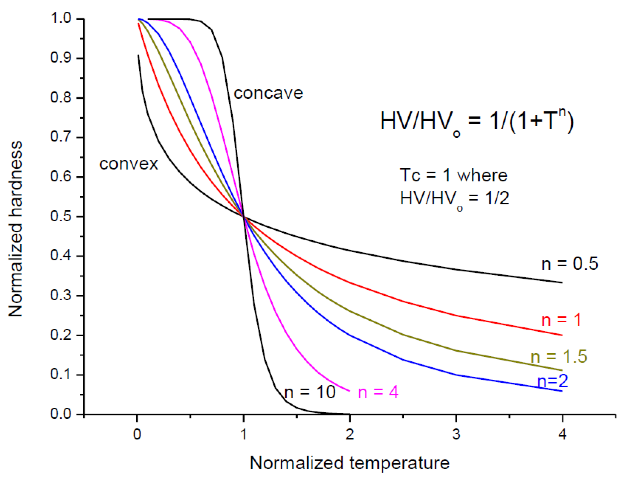
It should be mentioned that the two expressions mutually exclude one another, although both represent an exponentially decreasing function. But the essential difference is that Equation (1) is convex and Equation (2) is concave in the majority of the temperature range between 0K and melting point, T_m. Choosing one of the two mathematical expressions (Equation (1) or (2)) means selecting between the physical processes behind the mathematical description. We will see that pure metals present a convex decay, whereas the HEAs with a substantial stored elastic energy show a concave decay. However, both pure metals and alloys present convex decay near to absolute zero temperature. All the metals and alloys present a slow decrease at low temperatures. The hardness of pure metals starts an exponential decay already before room temperature, whereas, for alloys, the slow decay of hardness extends up to several 100 degrees. Sherby and Armstrong [16] and Merchant et al. [17] applied the Arrhenius-type Equation (2) for the determination of the activation energy. The contradiction between the two formulas was solved, apparently, by taking into account the data obtained at high temperatures only, above T_m/2. Certainly, if data were accurate and numerous enough to obtain a more exact fit, then the Arrhenius plot (lnH against 1/T) would be a curve instead of a straight line, resulting in a gradually changing activation energy.

Recently, based on one energy method [18], a formula has been presented to describe the temperature dependence of hardness without free parameters. The ratio of hardnesses relative to the reference hardness at room temperature, To, was given as [18]:

$$H(T)=H(T_o)\cdot {\left[{\displaystyle \frac{E(T)}{E(T_o)}}\left(1-{\displaystyle \frac{T-T_o}{T_m-T_o}}\right)\right]}^{1/2}\cdot {\left[{\displaystyle \frac{h(T_o)}{h(T)}}\right]}^{1/3}$$

(3)

where Tm is the melting temperature, h represents the indentation depth and E(T) is the Young’s modulus.

A very similar formula was presented for ceramics [19]:

$${\displaystyle \frac{H(T)}{H(T_o)}}={\left[\left({\displaystyle \frac{E(T)}{E(T_o)}}\right)\hspace{0.17em}\cdot \left({\displaystyle \frac{T_m-T}{T_m-T_o}}\right)\right]}^{1/2}$$

(4)

In order to apply Formulas (3) and (4), one need, besides the experimental data of indentation depth ratios, h(T_o)/h(T), the a priori knowledge of Young’s moduli ratios, E(T)/E(T_o).

Concerning the Young’s modulus, the following equation proposed by Wachtman et al. (1961) [20] is one of the most frequently used temperature-dependent Young’s modulus models:

$$E=E_o-B_{1}T\exp (-To/T),$$

(5)

where E_o is the Young’s modulus at absolute zero. B₁ is the slope of Young’s temperature curve in the high temperature range. T_o is a material parameter correlated with the Debye temperature.

A more recent paper on a temperature-dependent elastic modulus model for metallic bulk materials was published by Weiguo Li et al. [21]:

$${\displaystyle \frac{E(T)}{E(T_o)}}={{\displaystyle \frac{\left(1+{\displaystyle \underset{0}{\overset{T_o}{\int }}\alpha (t)dt}\right)}{{\left(1+{\displaystyle \underset{0}{\overset{T}{\int }}\alpha (t)dt}\right)}^3}}}^3\times {\left(1-{\displaystyle \frac{T-T_o}{T_m-T_o+\frac{{\Delta }_{fus}H}{C_v}}}\right)}^{1/2}$$

(6)

where ${\Delta }_{fus}H$ is the latent heat of fusion and C_v is the Debye integral [22] which, at the high-temperature limit (T >> θ_D) is C_v = 3N_o·k_B = 3 R = 25 J/mol·K, in agreement with the Dulong–Petit law.

It is interesting that the formula of Overton and Gaffney [23] who divided the temperature dependence into two, as well as the softening coefficient, also introduced the linear expansion coefficient. Unfortunately, their discussion remained on the level of elastic constant only.

$${\displaystyle \frac{C_{44}(T)}{C_{44}(0K)}}={\displaystyle \frac{\exp (-B\cdot \alpha (t)\cdot T)}{(1+{\displaystyle \underset{0}{\overset{T}{\int }}\alpha (t)\cdot dt{)}^9}}}$$

(7)

We mention that the Young’s modulus is size-dependent [23,24], which is important in the preparation of nanocomposites, but this is beyond the scope of our current topic.

The purpose of this paper is to check these “old” formulas using datasets from the literature and to contribute to the hot hardness problem with new formulas checked with more recent literature data and some of our own data obtained with a home-built instrument. Based on the datasets from the literature and from our own measurements, we present the application of the “old” Ito formula (Equation (1)) and two new, rational type, own formulas (Equations (11) and (20)). Then, we will apply in our new edition, the Arrhenius-type relation (Equation (2)) in the upper part of the temperature domain region in order to determine and apply the activation energy. Finally, we present our “universal” formula (Equation (21)), applicable in the whole temperature domain, for alloys.

2. Experimental

A schematic drawing of the instrument (see more details in [4]) is presented in Figure 1.

The indentation depth of a tungsten tip into the sample is measured as a displacement of a unit consisting of the sample and indenter, their captures and the indenter guide. Variable load (between 0.1 and 3 kg) can be applied to compress the tip into the sample. Around the unit, a tubular furnace can be mounted, which provides a high heating rate of 35 K/min up to the 1100 °C: the maximum working temperature. Starting a temperature scan from room temperature initially, up to several 10 degrees, the unit expands due to thermal dilatation (positive displacement is measured). The developing indentation depth turns the displacement negative. The indentation depth (ID) will be obtained by subtracting the displacement (D) from the linearly extrapolated initial thermal expansion (TEL): ID = TEL-D. The Rockwell-type hardness parameter, HR, will be obtained by subtracting the indentation depth from an arbitrarily chosen number, N (N > ID). Usually, we take an integer near the maximum value of ID. In this way, we turn an increasing ID parameter into a decreasing HR parameter:

HR = N − ID.

(8)

3. Results

3.1. Critical Review of the Formulas Without Fitting Parameters

Apparently, the Formulas (3)–(6) solve the problem of fitting the high-temperature hardness behavior of materials, moreover, without fitting parameters. A closer look at some of the prior datasets reveals that the temperature dependence of the thermal expansion coefficient, of the specific heat capacity and of the Young’s modulus need to be added. We examine the effects of these factors by making simplifications, trying to use acceptable approximations.

Formula (6) can be simplified as follows: The linear temperature expansion coefficient we can approximate by 0.022/Tm ((Equation (8)) in [25]); the first part of the expression (6) becomes, after simplification:

$${\left({\displaystyle \frac{1+0.022\frac{T_o}{T_m}}{1+0.022\frac{T}{T_m}}}\right)}^3={\left({\displaystyle \frac{1+0.022\frac{300}{1800}}{1+0.022\cdot 1}}\right)}^3=0.947.$$

(9)

where we have supposed the reference temperature as T_o = 300 K and an average melting temperature T_m = 1800 K; 1800 K can be considered the lowest value of the temperature region of refractory materials, and correspondingly the result is the highest error.

Neglecting this term, the error is less than 6%.

Concerning the second term, we first evaluate the characteristic temperature resulting from the ratio of heat of fusion and specific heat for 30 elements (see

Table 1. Dataset for the calculation of characteristic temperature Ts = Q/C and for the base value of hardness, H = 0.5Q/V_m.

Element	Tm	C	Q	Q/C	Vm	Hexp	Hcalc
-	K	J/mol∙K	kJ/mol	K	cm3/mol	Kgf/mm2	Kgf/mm2
Al	933.5	24.2	10.71	442.56	9.99	25	53
Au	1338	25.4	12.65	497.68	10.21	20	61
Ag	1234	25.35	11.28	444.97	10.38	25	54.35
Zn	692.7	25.39	7.32	288.30	9.157	35	39.9
Ir	2716	26.74	41.12	1537.8	8.513	200	241.5
Co	1768	24.81	16.06	647.32	6.622	104	121.2
Mg	923	24.469	8.48	346.56	13.98	26	30.3
Mn	1519	26.32	12.91	490.50	7.354	100	87.7
Mo	2896	24.06	37.48	1557.8	9.334	210	200
Ni	1728	26.07	17.48	670.50	6.589	63	132
Pb	600.6	26.65	4.77	178.99	18.27	4.5	13.05
Sn	505	27.112	7.03	259.29	16.24	6.2	21
Pd	1825	5.98	6.74	644.34	8.851	50	94.57
Pt	2045	25.86	22.17	857.31	8.629	47	128.5
Cu	1358	25.36	13.26	522.87	7.092	35	91.85
Ta	3258	25.36	36.67	1446.0	10.87	105	168.3
Fe	1809	25.1	13.81	550.20	7.082	61	97.35
W	3680	24.27	52.31	2155.3	9.55	345	273
Os	3300	24.7	31	1255.1	8.687	350	333
Ti	1939	25.06	18.7	746.21	10.32	85	94.16
Zr	2125	25.36	21	828.08	14.01	130	50
Hf	2500	25.73	27.2	1057.1	13.41	180	101.4
V	2190	24.89	21.5	863.80	8.337	83	129
Nb	2750	24.6	30	1219.5	10.84	110	138
Cr	2130	23.35	21	899.36	7.232	106	146
Re	3453	25.48	33	1295.1	8.859	135	186.8
Ru	2523	24.06	25.7	1068.2	8.171	216	236
Rh	2233	24.98	26.59	1064.5	8.345	110	159

and Figure 2). Surprisingly, this characteristic temperature turns out to be equal to half of the melting temperature, where the softening of red hardness starts. By heating up the sample to T_m/2, one would compensate for the latent heat of fusion lost exothermically during the solidification. One is tempted to argue that the hardness of the material originates in the process of solidification from the liquid phase. This conjecture is further supported by Figure 3, where the relationship between the hardness of pure elements and their heat of fusion, Q, presents an acceptable good correlation. We emphasize that this is the base hardness value valid for pure elements, if possible, in a single crystal state. In practice, we have to deal with a number of hardness-increasing factors, like grain size, precipitations, phase mixture, solid solution, etc., which may increase the hardness 3–4 times compared to the base value.

These tabulated T_m, C, Q_fus, V_m and H_exp data were taken from periodictable.com and knowledgedoor.com sites.

Based on the relation presented in Figure 3, we replace Q_fus/C = 0.5T_m in the second factor of Equation (6), and after some algebra we obtain the following simplified form:

$${\left(1-{\displaystyle \frac{T-T_o}{T_m-T+\frac{Q_{fus}}{Cv}}}\right)}^{1/2}={\left(1-{\displaystyle \frac{T-T_o}{1.5T_m-T_o}}\right)}^{1/2}={\left({\displaystyle \frac{1.5\frac{T_m}{T_o}}{1.5\frac{T_m}{T_o}-1}}\right)}^{1/2}\cdot {\left(1-{\displaystyle \frac{T}{1.5T_m}}\right)}^{1/2}$$

To obtain an order of magnitude result, we approximate T_o = 300 K and T_m = 1800 K, then the numerical part of the second factor will be (10/9)^0.5 = 1.0545. Interestingly, the two numerical factors compensate for one another (0.947 × 1.06 ~1), and the temperature variation of the Young’s modulus reduces to:

$${\displaystyle \frac{E(T)}{E(T_o)}}={\left(1-{\displaystyle \frac{T}{1.5T_m}}\right)}^{1/2}.$$

(10)

Coming back to Equation (4) of the hardness:

$${\displaystyle \frac{H(T)}{H(T_o)}}=\sqrt{1-{\displaystyle \frac{T}{1.5*T_m}}}\sqrt{{\displaystyle \frac{T_m-T}{T_m-T_o}}}=\sqrt{1-{\displaystyle \frac{T}{1.5*T_m}}}\sqrt{{\displaystyle \frac{T_m}{T_m-T_o}}}\sqrt{1-{\displaystyle \frac{T}{T_m}}}$$

The numerical factor can be approximate as:

$$\sqrt{{\displaystyle \frac{T_m}{T_m-T_o}}}={\left({\displaystyle \frac{T_m/T_o}{T_m/T_o-1}}\right)}^{1/2},$$

where T_o ~ 300 K, the average T_m ~ 1800 K and the numerical factor becomes (6/5)^^1/2 = 1.095, less than 10% error if we retain the following factors only:

$${\displaystyle \frac{H(T)}{H(T_o)}}=\sqrt{1-{\displaystyle \frac{T}{1.5*T_m}}}\sqrt{1-{\displaystyle \frac{T}{T_m}}}.$$

(11)

This is a universal valid function depending on the homologue’s temperature, T/T_m, only and is a linear decreasing function up to T_o/T_m ~ 0.8, as one can see in Figure 4. This almost linear dependence is also visible from the experimental data presented for alloys and composites in [21], which were carried out only up to 800 °C, which does not exceed 60% of the melting point, so we expect a linear relationship according to the simplified formula (Equation (11)).

Equation (11) should be further simplified because, in practice, the melting point is not always known; eventually an approximate value can be obtained by the rule of mixture from the melting points of the constituents. The last simplified version is Equation (12), which contains two parameters only: an exponent n < 1 and a characteristic temperature T_c not far away from the melting point T_m. The fitting result is shown in Figure 5.

$${\displaystyle \frac{H(T)}{H(T_o)}}={\left(1-{\displaystyle \frac{T}{T_c}}\right)}^n$$

(12)

It turns out that the hardness Formulas (3) and (4), without fitting parameters but with a priori knowledge of temperature dependences of the Young’s modulus, of the linear thermal expansion and of the indentation depth, could be replaced with a semi empirical formula with two fitting parameters only and no a priori knowledge; only the temperature dependence of relative hardness data is needed.

3.2. Critical Review of the Formulas with Fitting Parameters

First, we gather together the old and new formulas we are going to apply for the temperature dependence of hardness. There are essentially two types of temperature dependence: concave and convex. In general, pure metals present convex forms, whereas alloys always show concave dependencies. After the compilation of the formulas, we will apply them to some representative metals. In addition, we will study the activation energies obtainable in high-temperature regions, near to the melting point.

3.2.1. Formulas for Pure Metals—Convex Case

As well as the application of the Ito formula, we will also present two of our own formulas (Equations (14) and (20)) in order to extract further information concerning the temperature dependences of pure metals.

The Ito formula (Equation (1)) is a phenomenological expression valid for decay-type dependences (convex curve), which is characteristic for pure metals only. Several authors have presented the fittings with Ito’s formula [13,17]. They have used two temperature sections of the data, with two sets of characteristics: A1–B1 and A2–B2. To simplify the presentation, we will use a ratio of hardness relative to a reference value, and, instead of “softness coefficient”, B, we will use the reciprocal, which is the softening temperature, T_s1 = 1/B₁.

Processing the data of these authors, we first plotted the reciprocal values of the softening coefficients as a function of T_m (see Figure 6), and this method showed that T₁ = 1/B₁ is very close to 0.5 T_m. T₂ was much smaller (T₂ = 0.128 × T_m); therefore, it cannot be called a softening temperature in any way.

In order to find a correlation between the Ito formula (Equation (1)) and our own (Formula (12)), we expand in Taylor series both expressions (see Equations (13) and (14)), where, from an approximate value of the T_m can be estimated T_m = 2.27 × T_s. The characteristic temperature T₁ = 0.44 × T_m, from Figure 6, was taken as the softening temperature T_s, (T_s = T₁).

$${\displaystyle \frac{H(T)}{H(T_o)}}=\exp \left(-{\displaystyle \frac{T}{T_s}}\right)~1-{\displaystyle \frac{T}{T_s}}$$

(13)

$${\displaystyle \frac{H(T)}{H(T_o)}}={\left(1-{\displaystyle \frac{T}{T_C}}\right)}^n~1-n{\displaystyle \frac{T}{T_C}}$$

(14)

$$\begin{gathered} T_S={\displaystyle \frac{T_C}{n}} \\ \mathrm{and} T_m ~ 2.27 \times T_s = 2.27 \times T_c/n. \end{gathered}$$

(15)

It turns out that, whenever fitting with Formula (12) is possible, the melting point can be estimated from the fitted Tc and n parameters. The validity of this finding can be checked using the experimental data of pure metals [17].

In a recent paper [25], we presented a simple expression between the hardness of pure metals and their shear modulus:

HV_(kgf/mm²₎ = 1.67 × G_(GPa).

(16)

Furthermore, we have established a simple correlation between the shear modulus, G, and two basic parameters the G depends on: the metallic valence, Z, and the metallic atomic radius, R:

G_(GPa) = 14 Z²/R⁴_(A)

(17)

Increasing the temperature, the atomic bond is weakened by the elongation of interatomic distances and by the decrease of overlaps between the unpaired d orbitals. The former is a simple thermal expansion:

R = R_o(1 + α × T),

(18)

whereas the latter can be taken as the decreasing of effective metallic valence:

Z = Z_o (1 – B × T):

(19)

Finely, in addition to Ito’s exponentially decaying function (see Equation (1)), we will apply the following rational expression with only three parameters to be fitted:

H = H_o(1 – B × T)²/1+ α × T)⁴.

(20)

This fractional expression has meaning only if the numerator becomes zero well above the melting point (T_z = 1/B is a new characteristic temperature that has to correspond to the relation T_z > T_m). It should be noted that the rather arbitrarily taken numerator is nothing else but the Taylor expansion and the exponentially decaying function. So, Equation (20) is practically a modified Ito formula, where the denominator represents only a factor of (1 + 0.22*T/T_m)⁴ = 1.09 for T = T_m, which differ from a factor of 1 by only 10%. Here, the average value of linear thermal expansion, α = 0.022/T_m, was considered, as in Equation (8) in [25].

3.2.2. Formula for Alloys-Concave Case

In general, the pure metal temperature dependence is convex, whereas the alloys present concave dependences. Looking for a general formula valuable for both convex and concave cases, we came across Equation (21), which has a number of advantages: (1) applicable for both convex and concave forms, (2) for T = T_c, the hardness is halved, helping to predict the extent of the high-temperature region.

$${\displaystyle \frac{H(T)}{H(T_o)}}={\displaystyle \frac{1}{1+{\left(\frac{T}{T_c}\right)}^n}}$$

(21)

To facilitate the understanding of Equation (21), we present it in normalized form in Figure 7, taking Tc = 1. One can follow the change of concaveness with increasing exponent above n = 1 and increasing convex character with decreasing exponent below n = 1.

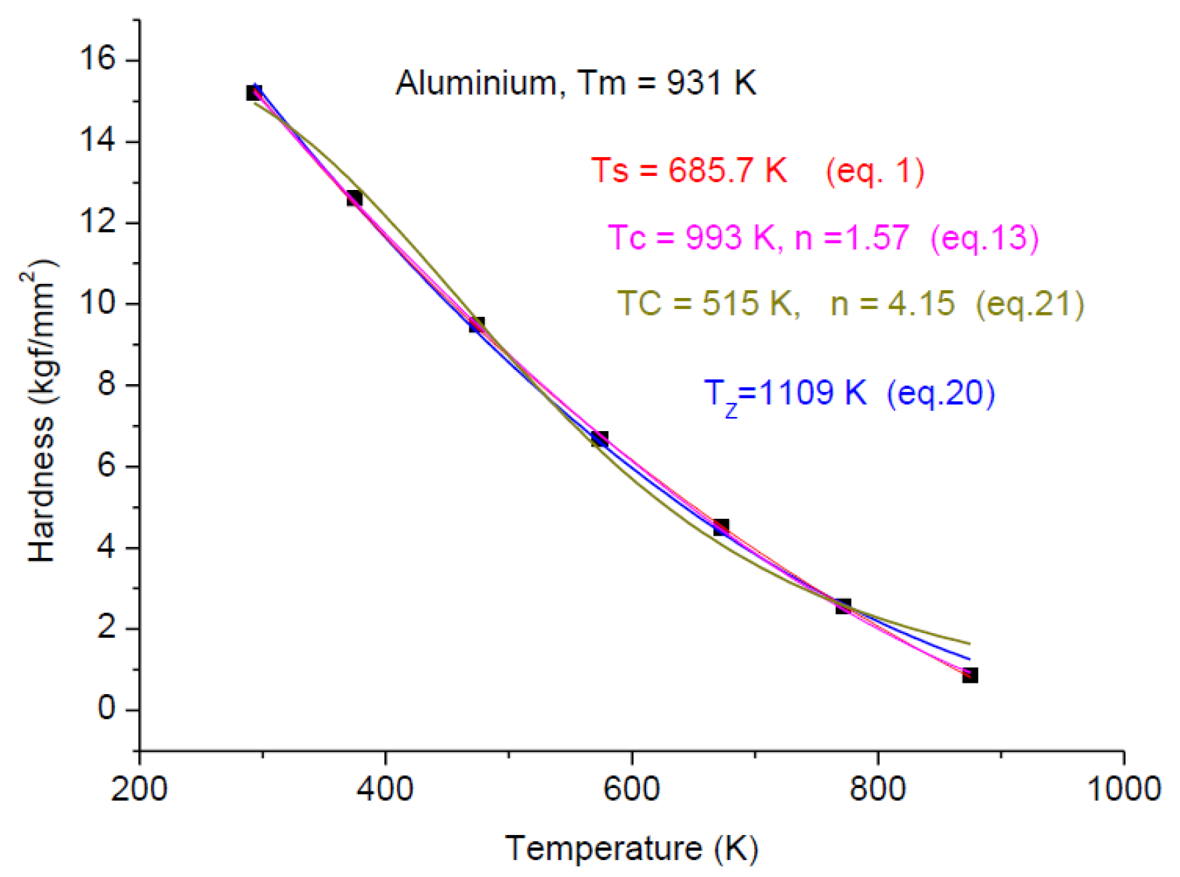
4. Examples of Pure Metal Applications

In the following, we are going to apply Formulas (1), (12), (20) and (21) for pure metals for which H(T) data were obtainable in the literature.

In Figure 8, Figure 9 and Figure 10, we present the temperature dependence for three pure metals, which belong to FCC, HCP and BCC structures, demonstrating that these four fittings (Equations (1), (13), (20) and (21)) are applicable independent of the crystalline structure. However, mathematical applicability does not mean physical applicability as well. For Aluminum, we obtained meaningful characteristic temperature values, but in the case of Magnesium, we have obtained unacceptably low T_s and T_z values. T_z is less then T_m (it should be larger), and T_s and T_c should be around T_m/2. For T_c = 357 K, H = 0.5H_o, as is expected. 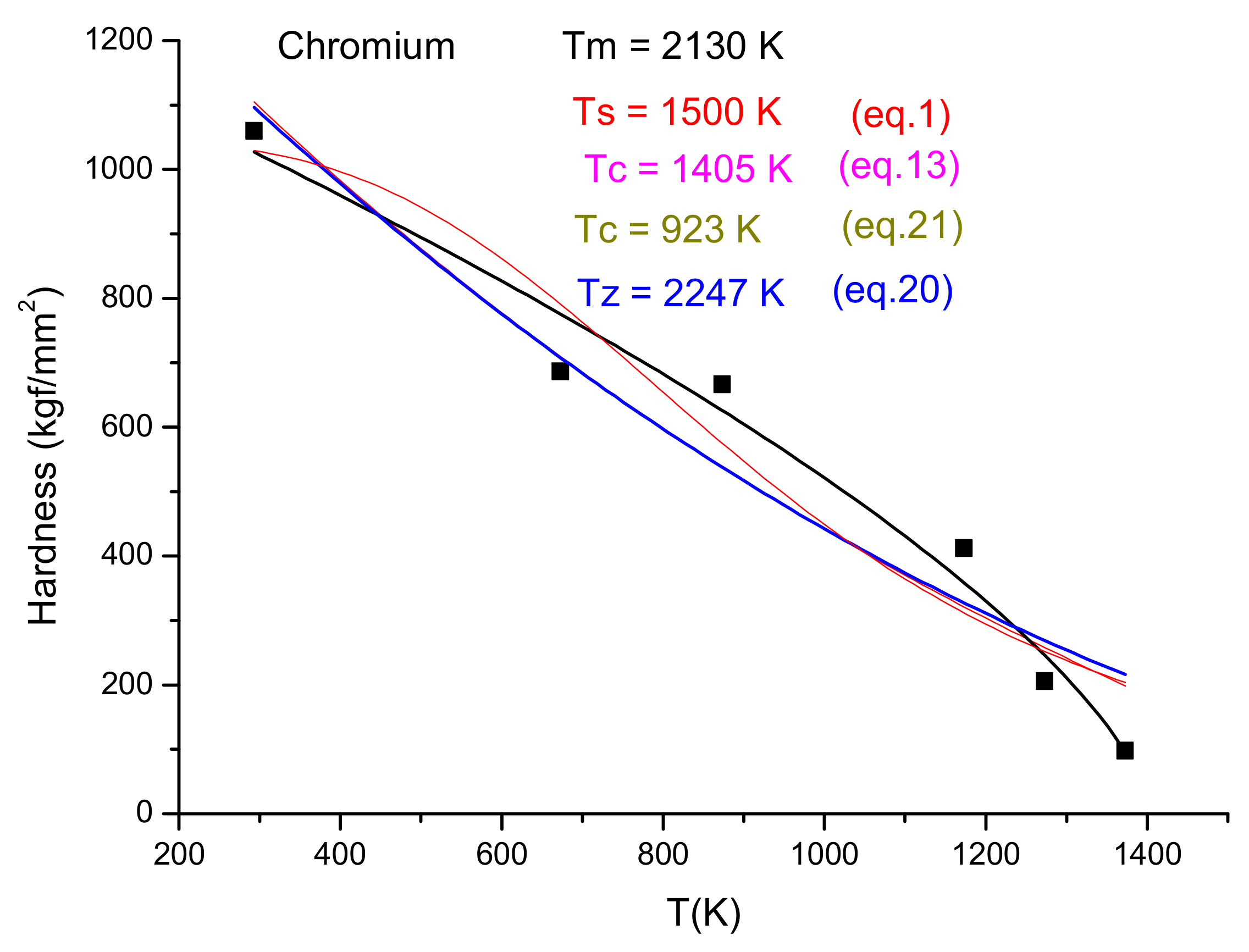The only meaningful data are the T_c value from Equation (21), which determine that the only meaningful formula applicable for Magnesium is the currently introduced formula: Equation (21). Chromium in Figure 10 is at the border of the concave–convex cases. The fitting quality drops from R² ~ 0.9 down to R² ~ 0.8. This quality loss is due to the scattering of the hardness data. It turned out that it is much more difficult to provide “pure” specimens from early transition elements (ETM) then from late transition elements (LTM). ETM samples are easily contaminated with H, C and especially oxygen, changing the hardness values. The heat treatments, even at the lowest temperature, should be done in an inert oxide powder bed (e.g., Cerium oxide).

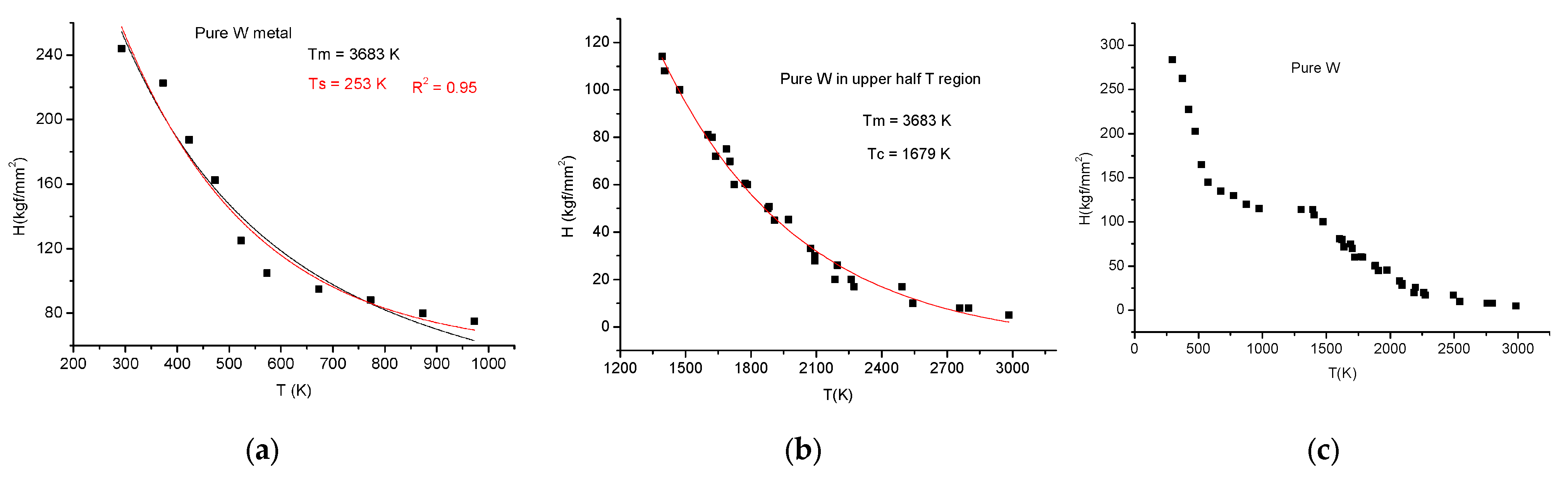
The situation is even more peculiar for Tungsten. We split the collected data from [27,28,29] in two, corresponding to the lower half (see Figure 11a) and upper half (see Figure 11b) temperature regions shown in Figure 11a,b. Tungsten presents a brittle-ductile transition above 500 K, not far away from room temperature. Certainly, the normal exponential decay is perturbed by this B–D transition.

Applying fitting in the lower half with Equations (1) and (21) (Equation (1) H(T) = 639 × exp(−T/253) + 55 and Equation (21). H(T) = 584/(1+(T/247)^1.54)), we obtained characteristic temperatures without physical meanings. None of Equations (13), (20) and (21) are applicable to describing the double decay feature of W hardness presenting a plateau around 1400 K (see Figure 11c).

Finally, we put together the two parts, and we observe a two-stage decrease of hardness, presenting a platoon around 1400 K. To the best of our knowledge, such behavior of W hardness and the explanation of it is missing in the literature. It is our conjecture that this behavior stems from the recrystallization, which occurs typically around 1400 K.

The goodness of fit is excellent for Equations (1) and (20) (R² = 0.99) and acceptable for the “universal” Equation (21).

The fitting with Equations (1) and (21) provided some characteristic temperatures near to half of the melting point for Equation (21) and around the (¾)*T_m for Equation (1). These temperatures are considered to signalize the change in the plastic deformation mechanism, but their value depends so much on the scattering of the hardness data that it is better not to attach any special importance to them. It is interesting that, based on Equation (20), we have got the linear expansion coefficient, within an order of magnitude, correct. Even more important seems to be the information about the decreasing of metallic valency, which seems to be an order of magnitude faster than the expansion. This should be a starting point for an ab initio study.

Silicon (see Figure 12) represents a curiosity: around a 623–700 K phase transformation occurs [30], named “indentation metallization”, which manifest itself as a rapid exponential decay of hot hardness. The original authors described the temperature dependence by two exponentials, whereas we describe it with one equation (Equation (21)). One can observe the perfect fit of the “universal” Equation (21) and the coincident of Debye temperature with the abrupt decrease of hardness. The transformation of covalent bonds into metallic ones, and the metallization, though very interesting, is beyond the scope of the present work.

5. Example for Alloy Applications

In Figure 13, a new application of “universal” Equation (21) is presented; fitting the hardness of the FCC, FCC + BCC and BCC phases produces the addition of Al into the HEA alloy originally composed of CrCoCuFeNi. The experimental data were compiled from [31,32]. The crystalline structure corresponds to the valence electron count (VEC) number: Al = 0, VEC = 8.8; FCC because VEC > 8, Al = 1, VEC = 7.8; FCC+BCC because 7.2 < VEC < 8, and for Al = 2, VEC = 7.14; BCC because VEC < 7.2.

Although only a few data points (only 6 or 7) are available, Equation (21) is able to describe the evolution of hardness in the whole temperature region up to melting. The parameters of fitting are as follows: For Al = 0.5: H_o = 415, T_c = 937 °C, n = 9.28. For Al = 1: H_o = 950 MPa, T_c = 632 °C, n = 6.47, and for Al = 2: H_o = 1615 MPa, T_c = 600 °C, n = 4.71. It can be observed that the BCC structure produces a room temperature hardness four times larger than the FCC structure; at high temperatures, this improvement is lost. This denotes similar indentation mechanisms at high temperatures, regardless of the crystalline structure.

6. Example for Activation Energy Determination, Arrhenius-Type Formulas

The only way to reconcile the mutually exclusive Equations (1) and (2) is to apply the exponential decay in lower-temperature regions and the Arrhenius-type equation for determining the indentation activation energy in high-temperature regions, above 3/4Tm. Unfortunately, the high-temperature data points are missing, because these are more difficult to determine. The logarithm of H versus T is not linear in most cases, so it is difficult to determine a single apparent activation energy. One can divide, rather arbitrarily, the T > Tm/2 temperature region into sub regions and determine the corresponding activation energies.

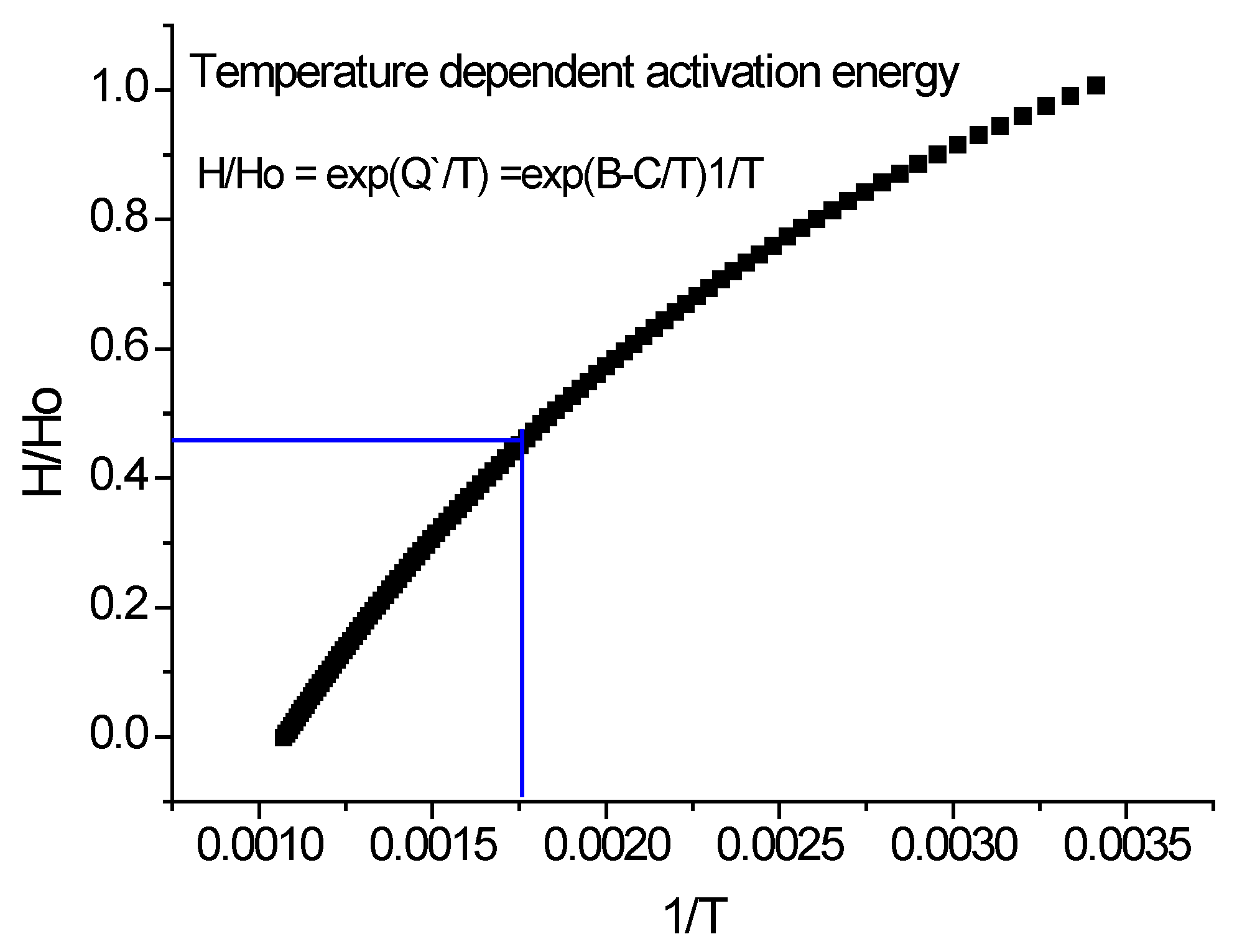
Here, we propose a more general valuable solution offering an apparent activation energy, Q’, which increases continuously from the starting temperature up to the melting point. To overcome the temperature-dependent apparent activation energy problem, we propose an Arrhenius-type expression for hot hardness with a temperature-dependent activation energy equation:

$$Q=B-C\cdot {\displaystyle \frac{1}{T}}$$

(22)

Applying Equation (22) for Q, we describe the variation of Q as a function of T; as expected, Q is small at small temperatures and large at higher temperatures. Varying Q represents a change in mechanism from the one controlled by the dislocation pipe diffusion at lower temperatures to the one controlled by lattice diffusion at higher temperatures.

In the following three figures (Figure 14, Figure 15 and Figure 16),we present how to calculate the parameters of temperature-dependent activation energy. Seven data points for Aluminum were taken from [26]. They present a normal convex exponential decay (see Figure 14), with a characteristic softening temperature at 675 K. After fitting, we have obtained 100 data points between room temperature and melting, T_m = 933 K. The more data points, the better the precision of the fitted parameters. The blue square in Figure 15 shows the high-temperature region, from where the apparent activation energy was determined.

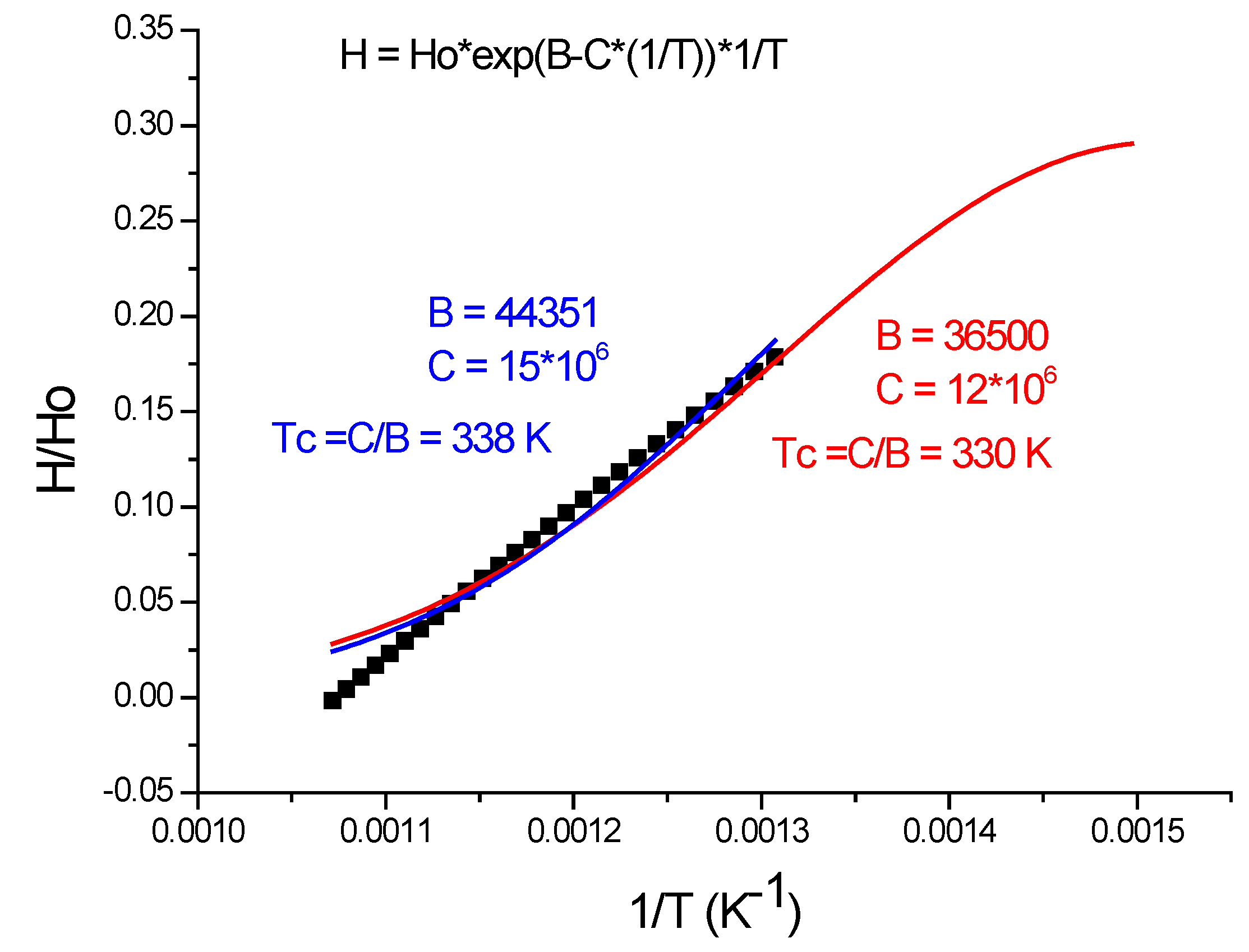
It is important to mention that expression (22) makes it possible to define a new characteristic temperature, where Q becomes zero at T_Q = C/B. This is the temperature where the activated dislocation motions start with increasing Q values as the temperature increases. In Figure 16, we have performed the fitting twice: first with 32 data point, shown by the red fitting line, and second we have used only 19 data point, shown by the blue fitting line. The results are similar (T_c = 330 or 338 K) and not strongly dependent on the number of data points.

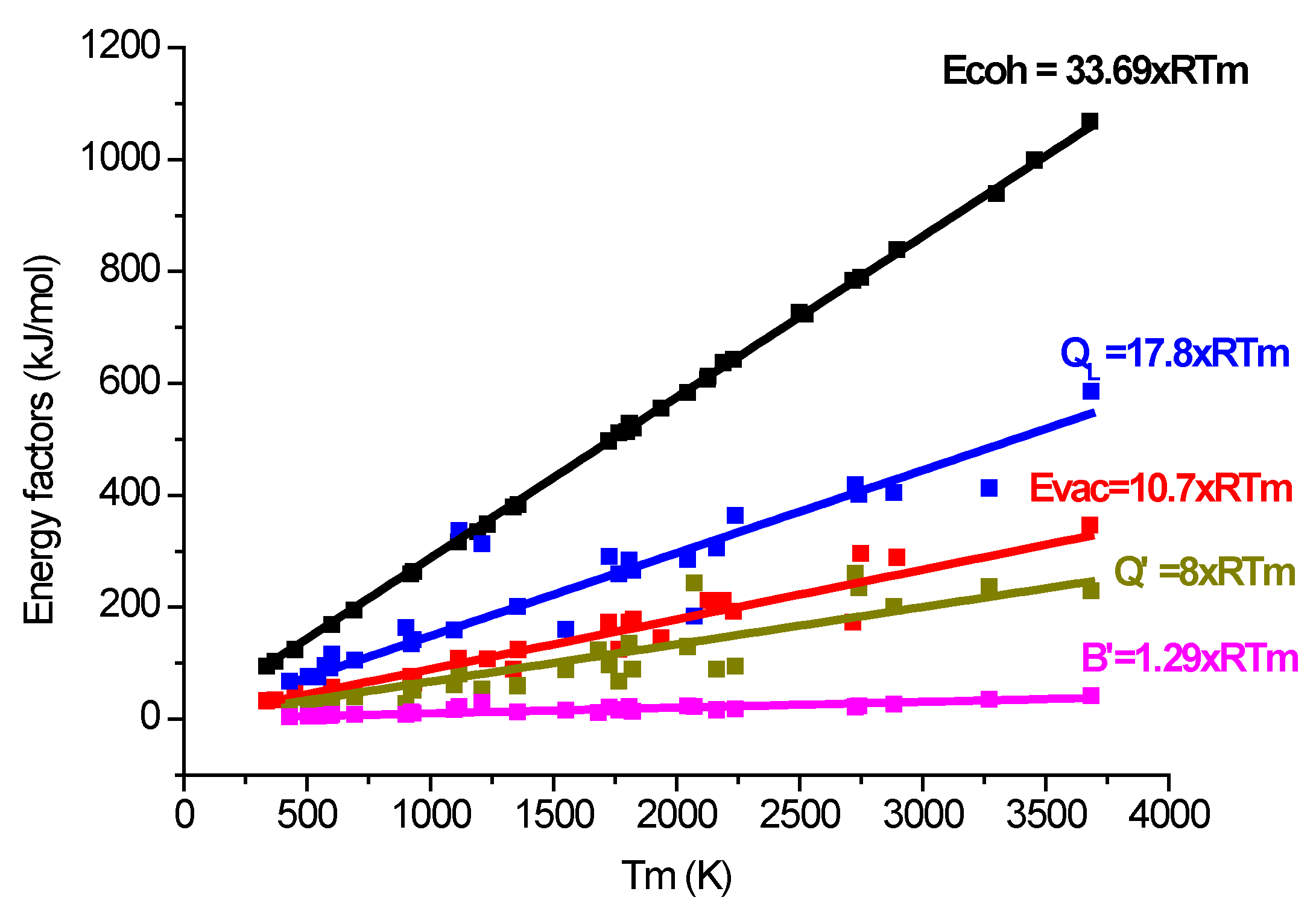
The maximal value will never surpass the value of self-diffusion activation energy. In order to facilitate a comparison of the activation energies, provided from the evaluation of hot hardness data and that of self-diffusion, we express the activation energy in RT_m units, where T_m is the melting point of the metal and R is the universal gas constant: Q = kRT_m. The high-temperature hardness expressed with apparent activation energy is:

H/Ho = exp(Q′/T)

(23)

Let us estimate the activation energy of hardness at high temperatures, near to the melting point where we simply approximate T with Tm (see Figure 17).

Then, we make equal the hardness values of exponential decays to the hardness expressed with the apparent activation energy in Equations (1) and (23):

B₂T_m = Q′/RT_m,

where B₂ = 1/T₂ and T₂ = 0.128T_m (see Figure 6). After some algebra, we obtain:

Q′ = 7.81 × RT_m

(24)

In Figure 18, as well as the “universal” valid activation energy, we have also represented the experimentally determined B′ (from [17]) apparent activation energy:

B′ = 1.29 × RT_m

(25)

The ratio is Q′/B′ ~ 6. Further research is necessary to find the relationship between indentation creep characteristics and these apparent activation energies. It is promising that these apparent activation energies are smaller than the energies necessary for vacancy formation, and for self-diffusion (see Figure 18).

These general valid apparent activation energies (Equations (24) and (25)) help in the estimation of hardness at high temperatures near to the melting point.

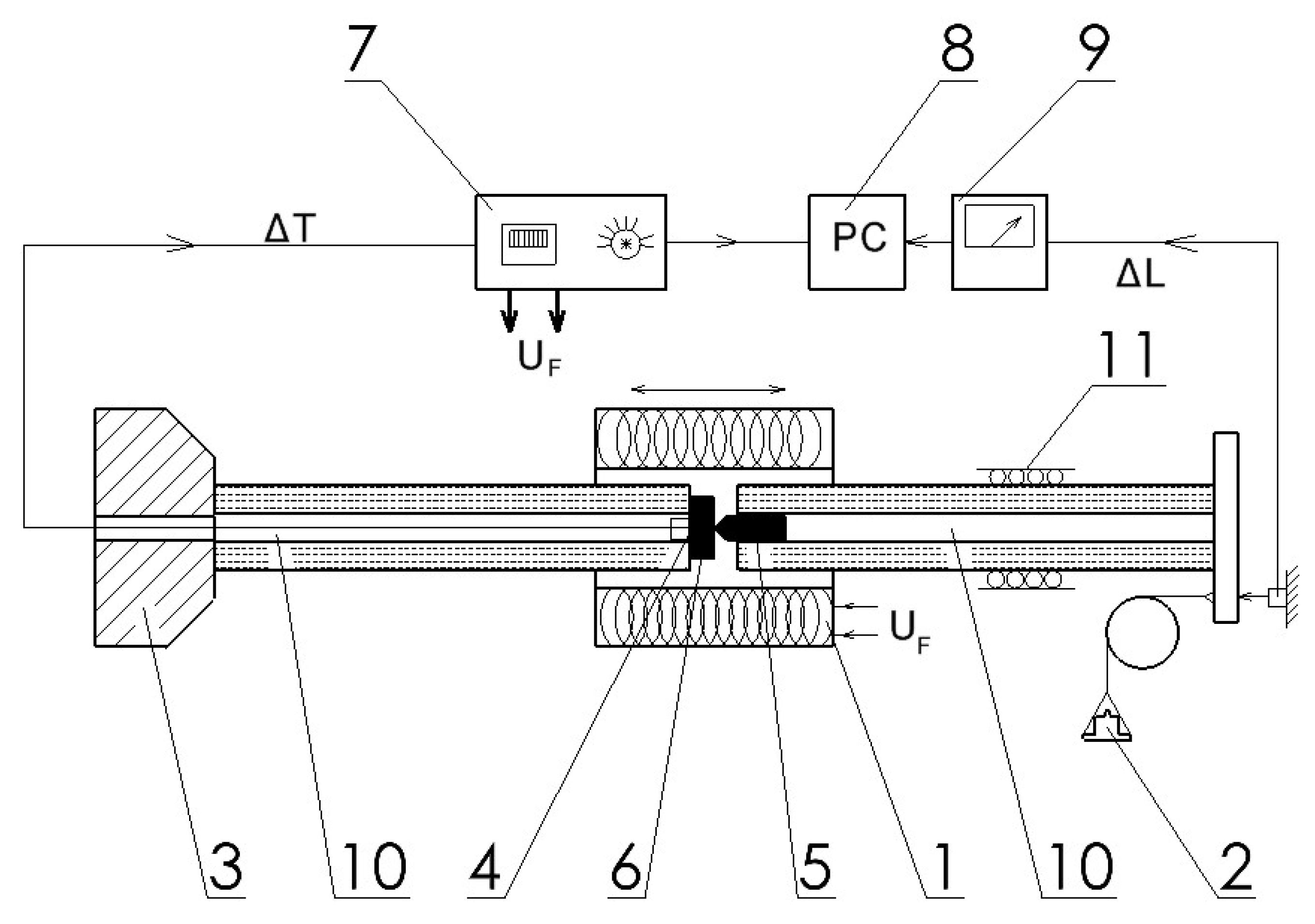
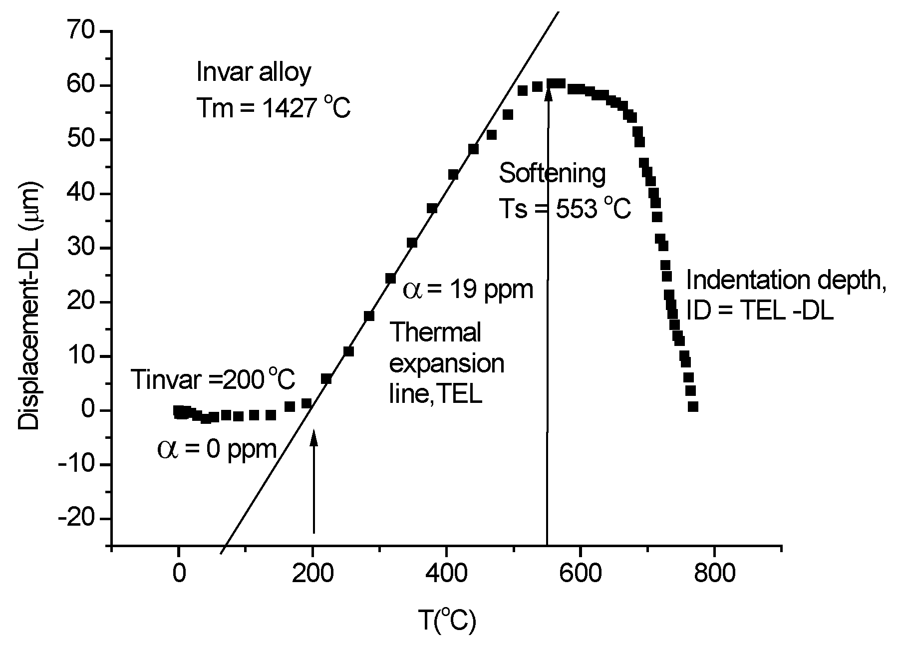
7. High Heating Rate Rockwell-Type Hardness Measurements

First, we present the evaluation procedure of the high heating rate indentation measurement using the home-built device presented in Figure 1. For this purpose, we have selected the invar alloy because it reveals the characteristics of the measurements: it shows zero thermal expansion up to 200 °C and then the thermal expansion separates from the indentation, which helps in determining the thermal expansion line (TEL)(see Figure 19) and the indentation depth as ID = TEL − DL. The Rockwell-type hardness can be fitted with the universal Equation (21).

The standard way of Rockwell-type hardness measurement consists of two displacement curve measurements: one for a small load (0.5 kg in this case) and a second with a larger load (1.5 kg). The difference in these two curves will give the indentation depth (ID), and the hardness will be obtained (Figure 20) by subtracting the indentation depth from an arbitrarily chosen number. In some cases, the thermal expansion prevails at low temperatures and the indentation depth starts to manifest itself at higher temperatures only. In this case, we can skip the low-load DL measurement and replace it with the thermal expansion line (TEL), which, in the present case, is TEL = −80 + (175/440)*T. The indentation depth will be given as ID = TEL-DI and the Rockwell-type hardness will be HR = 300-ID. This time the arbitrarily chosen number is 300.

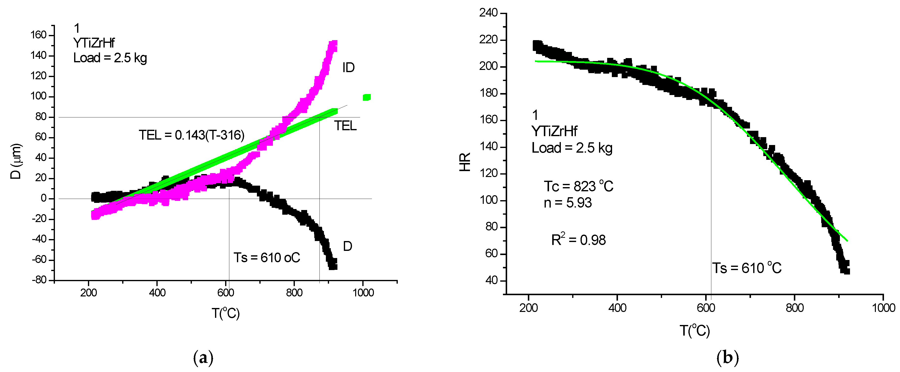
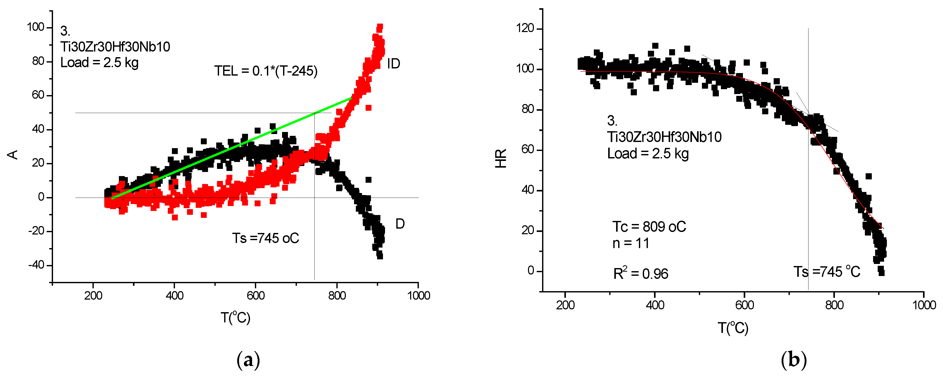
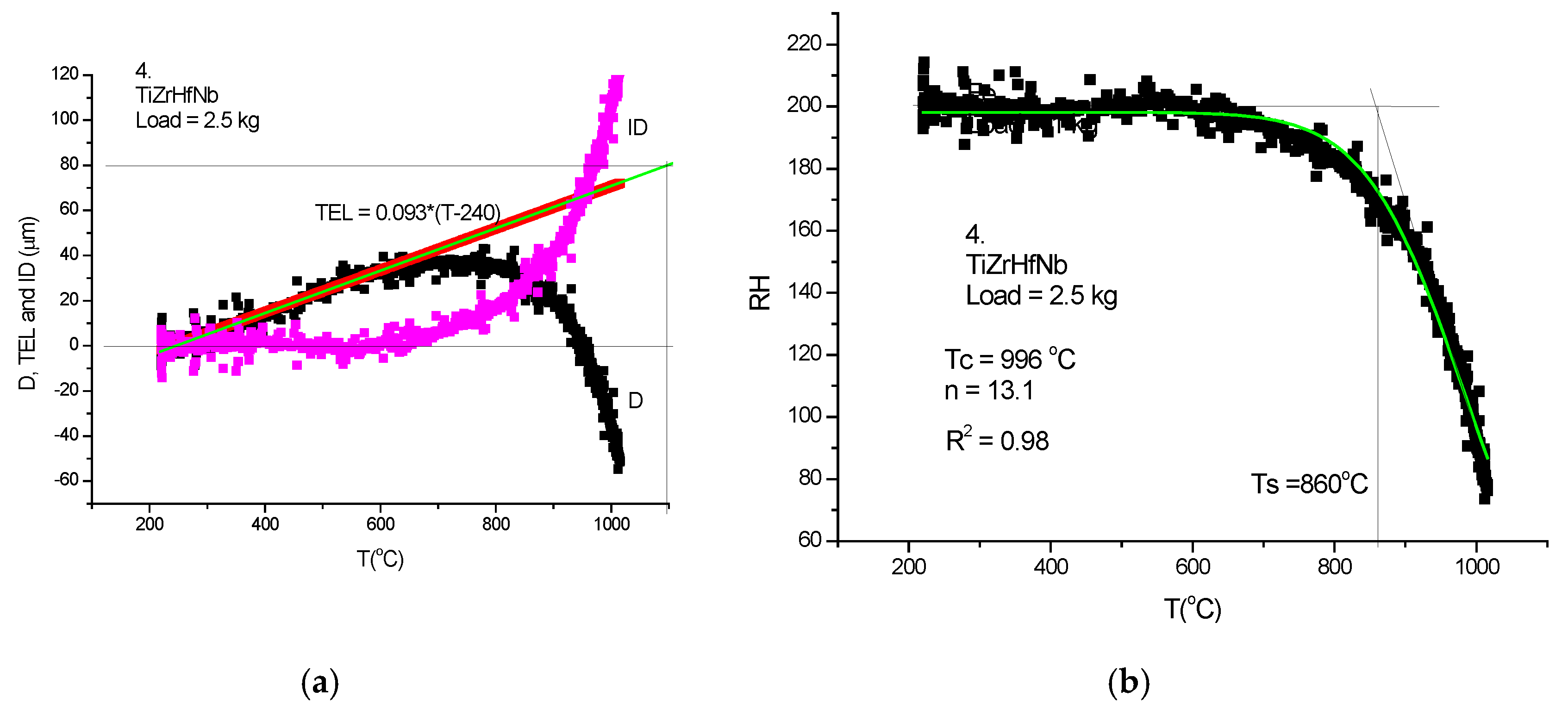
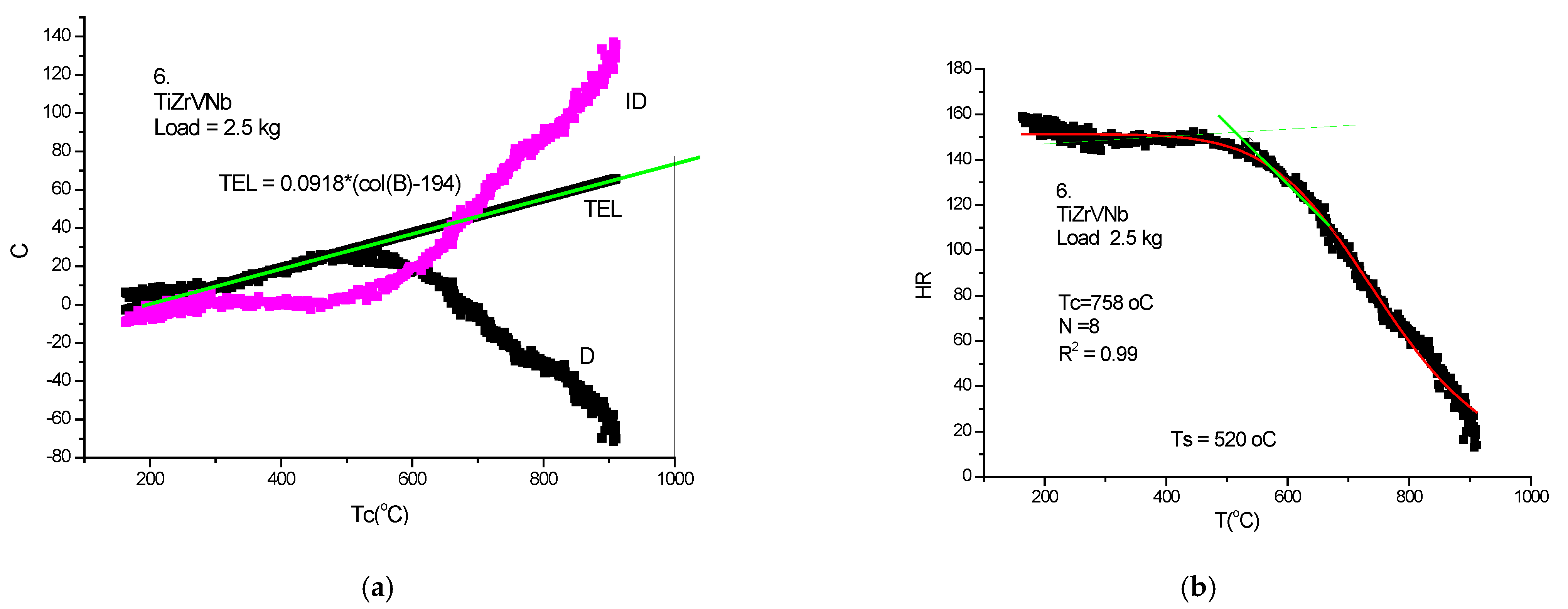
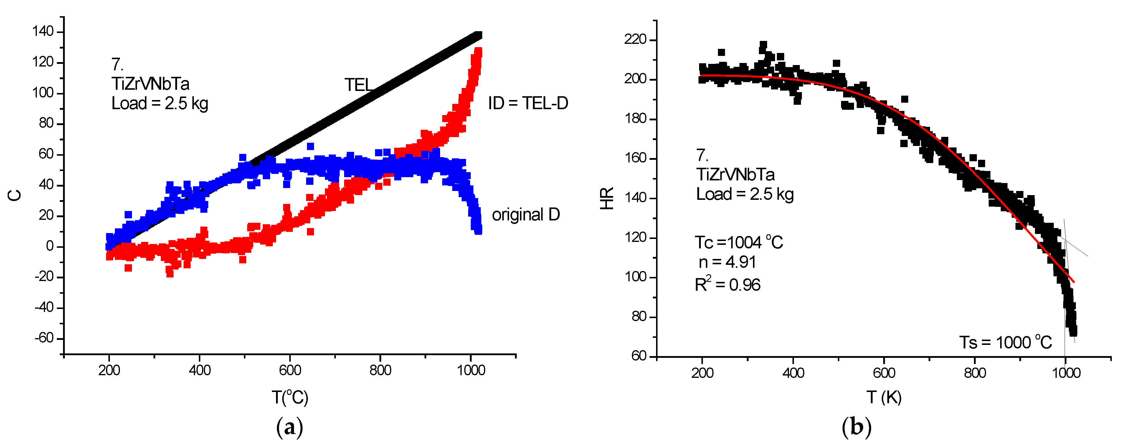
In the following, seven refractory high entropy alloys (RHEAs), compiled in

Table 2. Own design RHEAS and their fitted parameters.

	RHEA	Tmelting	Ts	Tc	n
	-	(K)	(°C)	(°C)	-
1	Y25Ti25Zr25Hf25	2093	610	823	5.53
3	Ti30Zr30Hf30Nb10	2247	722	803	11
4	Ti25Zr25Hf25Nb25	2329	860	996	13.1
5	Ti20Zr20Hf20Nb20V20	2296	744	830	10.8
6	Ti25Zr25V25Nb25	2244	520	758	8
7	Ti20Zr20V20Nb20Ta20	2454	1000	1004	4.91
8	V25Nb25Mo25W25	2874	1000	1250	12.5

, will be measured with our home-built equipment (see Figure 1) and commented on based on Figure 21, Figure 22, Figure 23, Figure 24, Figure 25 and Figure 26. The composition was selected to have VEC around the 4.2 value, which corresponds to minimum shear moduli. We have proceeded to use the thermal expansion line (TEL) and neglected the low load displacement line (DL). For all of the samples, we have applied the maximal heating rate of 35 K/min and the same load, F = 2.5 kg. The temperature scan is started at similar temperatures for all seven samples, and special attention is paid to observe and select the linear expansion part from where the TEL is determined. With increasing temperature, as well as the positive displacement of thermal expansion, appears the negative contribution of indentation depth (ID). ID should be calculated for the whole temperature interval. Then, this increasing ID function is transformed in a decreasing Rockwell-type hardness parameter. By subtracting it from an arbitrary sufficiently large number (N), all of the ID numbers are transformed into decreasing positive numbers:

HR = N − ID.

Although the figures satisfactorily explain the extraction of ID from the measured DL, some comments to the figures may help in “reading” the measured DL data. In Figure 21a, Figure 22a and Figure 23a, the linear expansion part is rather short, but was enough to obtain the ID. It is remarkable that the knee point at Ts, the temperature of softening, is more accentuated on the original DL (black) line then on the Rockwell-type hardness in Figure 21b, Figure 22b and Figure 23b. One can agree that, at the softening temperature, the negative IDs start to prevail upon the positive thermal expansion. This point can be identified as the end of the horizontal part of the displacement line. Altogether, the softening is not characterized by an inflexion point but rather by a smeared knee point. Comparison of initial DL and of the final RH parameters helps in defining the softening temperature, Ts.

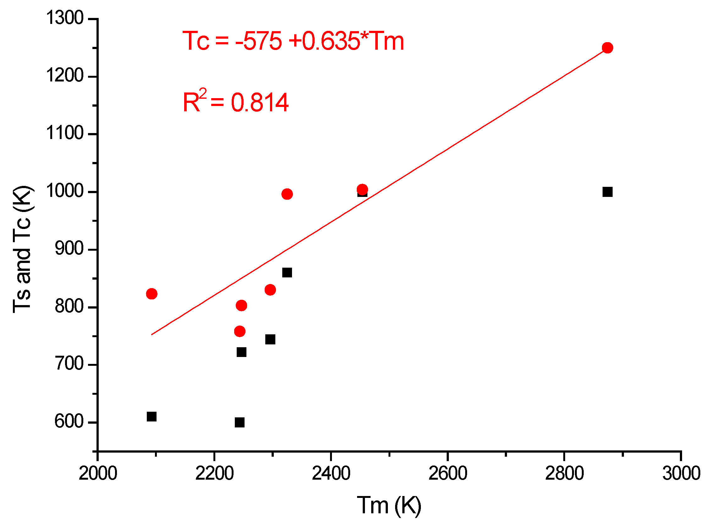
In Table 2, a compendium of the hot hardness characteristics (Ts and Tc) are presented as a function of Tm. Usually, the softening parameters Ts and Tc scale with the Tm/2. In the case of our RHEAS, however, this scaling is violated (see Figure 27) due to the phase instabilities produced by the allotropic transformation tendencies of Ti, Zr and Hf metals.

As a result, instead of Tm/2, the softening temperatures (Ts and Tc; see Figure 27) are better around Tm/3, which is smaller than the expected values for Ts and Tc (see example of pure metals applications (Figure 8, Figure 9, Figure 10 and Figure 11). A possible explanation for these discrepancies might be the phase instability of these Ti-, Zr- and Hf-containing RHEAs, which originate in the allotropic nature of these early transition elements. This phase instability manifests itself not only in the early softening but also in its room temperature crystalline structure, which in alloy is BCC, whereas in elemental form all three are HCP. It should be mentioned that BCC is the high-temperature allotropic form, and this preserves itself on cooling due to the alloying but transforms into HCP for elemental metal. Whenever one uses a light early transition element for obtaining low density alloy, one should be aware of the reduction of operational temperature, despite the high melting point of the alloy.

8. Conclusions

We found a series of relationships during the study of the temperature dependence of hardness: The hardness of pure, single-phase, elemental metals at room temperature can be obtained as the ratio of the heat of fusion to the molar volume, and the softening temperature can be obtained as the ratio of the heat of fusion to the specific heat capacity.

In addition to the exponential hardness-temperature H(T) dependence known from the literature, we introduced three new H(T) functions: 1. By expanding the exponential function, we created a rational H(T) function for pure metals. 2. Based on the dependence of hardness on the metallic valence and the metallic atomic radius, (H(T) = Z²/R⁴), we created a rational expression, where Z decreases linearly, while R increases linearly with temperature, and applied it to pure metals. 3. We have created a rational function with the power of the normalized temperature, which is universally suitable for describing the temperature dependence of both metals and alloys. 4. In the Arrhenius-type H(T) function, which is valid only at high temperatures, we have introduced and determined the temperature-dependent activation energy, which always remains smaller than the activation energy necessary for self-diffusion.

We have presented in detail the procedure of a measurement with our home-made rapid heating device: from the measured deformation measurement and the constructed thermal expansion line, we determined the indentation depth, and from that the relative hardness reminiscent of the Rockwell-type. During the measurements, we found that the alloys containing allotropic metals (Ti, Zr, Hf) show a much lower softening temperature than the expected Tm/2 value, just as the softening temperature of pure allotropic metals is adjusted to the temperature of the allotropic phase transition and not to the melting point.

Outlook

Hardness measurement at high temperatures may facilitate finding some correlations with corrosion and/or oxidation resistance [33], and in this way might contribute to the prolongation of life span of thermal power plants and nuclear reactors.

The temperature dependence of hardness has a decisive role in the wear resistance of alloys. Understanding the correlation between hardness and friction and wear as a function of temperature is a basic tribological problem [34].

One of the tasks of high-temperature hardness measurements is the study of creep [35] behavior in order to prolong the lifespan of gas turbine blades. Our equipment presented in Figure 1 is suitable for performing indentation creep or impression creep experiments on small samples several mm in size.

References

1. De Réaumur, R.A.F. Réaumur’s Memoirs on Steel and Iron: A Translation from the Original Printed in 1722; University of Chicago Press: Chicago, IL, USA, 1956. [Google Scholar]
2. Slavina, N.P.; Smirnov, A.V. Determining hardness at high temperatures. Meas. Tech. 1961, 4, 275–277. [Google Scholar] [CrossRef]
3. ONERA: “Office National d’Études et de Recherches Aerospace. They Perform Hot Hardness Measurements on Request”. Available online: https://www.element.com (accessed on 5 December 2023).
4. Temesi, O.K.; Karacs, A.; Chinh, N.Q.; Varga, L.K. Thermal Softening Measurements of Refractory High-Entropy Alloys. Materials 2024, 17, 5718. [Google Scholar] [CrossRef] [PubMed]
5. MFT 5000 Platform of Rtec Instruments, US 1810 Oakland Road, San Jose. Available online: https://www.stinstruments.com/mechanical-testing/indentation/high-temperature-hardness-tester/ (accessed on 2 August 2024).
6. Hot Hardness Testing on the UMT—Bruker, Nano Surfaces Division, Campbell, CA, USA. Available online: www.bruker.com/nanomechanical-testing (accessed on 12 January 2022).
7. Sikorova, G.; Chumakov, N.; Tumanov, M.; Zhikharev, S.; Panov, S. Hardness testing as a method to identify the highest-temperature combustion zone in transport fires. E3S Web Conf. 2023, 402, 11019. [Google Scholar] [CrossRef]
8. Shilin, C.; Wei, S. Analysis and Prediction of Hardness Change at High Temperature Based on BP Neural Network. In Proceedings of the 2023 IEEE 10th International Workshop on Metrology for AeroSpace (MetroAeroSpace), Milan, Italy, 19–21 June 2023; pp. 216–220. [Google Scholar] [CrossRef]
9. Rodriguez, S.; Lang, E.; Argibay, N.; Kustas, A.; Barrick, E.; Jones, M.; Arata, E.; Walker, C.; Monroe, G.; Whetten, S.; et al. Application of Refractory High-Entropy Alloys for Higher-Reliability and Higher-Efficiency Brayton Cycles and Advanced Nuclear Reactors; SAND2021-11377; Sandia National Laboratories: Albuquerque, NM, USA, 2021. [Google Scholar]
10. Liu, A.Y.; Cohen, M.L. Prediction of New Low Compressibility Solids. Science 1989, 245, 841–842. [Google Scholar] [CrossRef]
11. Yoshino, H.; Mézard, M. Emergence of rigidity at the structural glass transition: A first principle computation. Phys. Rev. Lett. 2010, 105, 015504. [Google Scholar] [CrossRef]
12. Teter, D.M. Computational Alchemy: The Search for New Superhard Materials. MRS Bull. 1998, 23, 22–27. [Google Scholar] [CrossRef]
13. Ito, K. Scientific Papers; Series 1; Tohoku University: Sendai, Japan, 1923; p. 137. [Google Scholar]
14. Schischokin, W. Die Härte und der Fließdruck der Metalle bei verschiedenen Temperaturen. Z. Anorg. Allg. Chem. 1930, 189, 263–282. [Google Scholar] [CrossRef]
15. Hsu, C.Y. Correlation of hot-microhardness with elevated temperature-tensile properties of low activation ferritic steel. J. Nucl. Mater. 1986, 141–143, 518–522. [Google Scholar] [CrossRef]
16. Sherby, O.D.; Armstrong, P.E. Prediction of activation energies for creep and self-diffusion from hot hardness data. Metall. Trans. 1971, 2, 3479–3484. [Google Scholar] [CrossRef]
17. Merchant, H.D.; Murty, G.S.; Bahadur, S.N.; Dwivedi, L.T.; Mehrotra, Y. Hardness temperature relationships in metals. J. Mater. Sci. 1973, 8, 437–442. [Google Scholar] [CrossRef]
18. Liu, Y.; Wang, R.; Wan, Y.; Zhou, S.; Cai, H.; Gu, M.; Li, D.; Li, W. Temperature-dependent hardness model of high-temperature materials can account for indentation size effect. Int. J. Refract. Met. Hard Mater. 2022, 108, 105957. [Google Scholar] [CrossRef]
19. Wang, R.Z.; Wang, X.R.; Li, D.I.; Li, W.G. A novel temperature dependent hardness model for high—Temperature structural ceramics. Ceram. Int. 2021, 47, 1462–1465. [Google Scholar] [CrossRef]
20. Wachtman, J.B.; Tefft, W., Jr.; Lam, D.G., Jr.; Apstein, C.S. Exponential temperature dependence of Young’s modulus for several oxides. Phys. Rev. 1961, 122, 1754–1759. [Google Scholar] [CrossRef]
21. Li, W.; Kou, H.; Zhang, X.; Ma, J.; Li, Y.; Geng, P.; Wu, X.; Chen, L.; Fang, D. Temperature-dependent elastic modulus model for metallic bulk materials. Mech. Mater. 2019, 139, 103194. [Google Scholar] [CrossRef]
22. Gu, M.X.; Sun, C.Q.; Chen, Z.; Au Yeung, T.C.; Li, S.; Tan, C.M.; Nosik, V. Size, temperature, and bond nature dependence of elasticity and its derivatives on extensibility, Debye temperature, and heat capacity of nanostructures. Phys. Rev. B 2007, 75, 125403. [Google Scholar] [CrossRef]
23. Overton, W.C.; Gaffney, J., Jr. Temperature variation of the elastic constants of cubic elements. Phys. Rev. 1955, 98, 969. [Google Scholar] [CrossRef]
24. Liang, L.H.; Li, M.Z.; Qin, F.Q.; Wei, Y.G. Temperature effect on elastic modulus of thin films and nanocrystals. Philos. Mag. 2013, 93, 574–583. [Google Scholar] [CrossRef]
25. Temesi, O.K.; Varga, L.K.; Chinh, N.Q.; Vitos, L. Prediction of the Cohesion Energy, Shear Modulus and Hardness of Single-Phase Metals and High-Entropy Alloys. Materials 2024, 17, 2728. [Google Scholar] [CrossRef]
26. Xu, N.; Li, W.; Ma, J.; Deng, Y.; Kou, H.; Li, Y.; Zhang, X. Modeling of Temperature-Dependent Hardness for Pure FCC and HCP Metals. Int. J. Appl. Mech. 2020, 12, 2050022. [Google Scholar] [CrossRef]
27. Borisenko, V.A. Relation between the hardness and strength of tungsten and molybdenum over a wide temperature range. Sov. Powder Metall. Met. Ceram. 1965, 4, 134–135. [Google Scholar] [CrossRef]
28. Krsjak, V.; Wei, S.H.; Antusch, S.; Dai, Y. Mechanical properties of tungsten in the transition temperature range. J. Nucl. Mater. 2014, 450, 81–87. [Google Scholar] [CrossRef]
29. Terentyev, D.; Xiao, X.; Lemeshko, S.; Hangen, U.; Zhurkin, E.E. High temperature nanoindentation of tungsten: Modelling and experimental validation. Int. J. Refract. Met. Hard Mater. 2020, 89, 105222. [Google Scholar] [CrossRef]
30. Domnich, V.; Aratyn, Y.; Kriven, W.M.; Gogotsi, Y. Temperature dependence of silicon hardness: Experimental evidence of phase transformations. Rev. Adv. Mater. Sci. 2008, 17, 33–41. [Google Scholar]
31. Tong, C.-J.; Chen, M.-R.; Yeh, J.-W.; Lin, S.-J.; Chen, S.-K.; Shun, T.-T.; Chang, S.-Y. Mechanical performance of the Al x CoCrCuFeNi high-entropy alloy system with multiprincipal elements. Metall. Mater. Trans. A 2005, 36, 1263–1271. [Google Scholar] [CrossRef]
32. Tong, C.-J.; Chen, Y.-L.; Chen, S.-K.; Yeh, J.-W.; Shun, T.-T.; Tsau, C.-H.; Lin, S.-J.; Chang, S.-Y. Microstructure Characterization of AlxCoCrCuFeNi High-Entropy Alloy System with Multiprincipal Elements. Metall. Mater. Trans. A 2005, 36A, 881–893. [Google Scholar] [CrossRef]
33. Wenga, T.; Macdonald, D.D.; Ma, W. Multi-scale computational study of high-temperature corrosion and the design of corrosion-resistant alloys. Prog. Mater. Sci. 2025, 148, 101359. [Google Scholar] [CrossRef]
34. Kumar, D. Recent advances in tribology of high entropy alloys: A critical review. Prog. Mater. Sci. 2023, 136, 101106. [Google Scholar] [CrossRef]
35. Li, W.; Xie, D.; Li, D.; Zhang, Y.; Gao, Y.; Liaw, P.K. Mechanical behavior of high-entropy alloys. Prog. Mater. Sci. 2021, 118, 100777. [Google Scholar] [CrossRef]
Figure 1. Schematic drawing of the instrument for indentation depth measurement. 1. Tube furnace that can be shifted; 2. Stressing load; 3. Fix point for indentation measurement; 4. Thermocouple; 5. Indenter; 6. Sample; 7. Power supply for heating; 8. Computer for data storage; 9. μm resolution inductive displacement sensor; 10. Rods and tubes made from quartz; 11. The guide, gliding on ball bearings.
Metals 15 00623 g001
Figure 2. Ratio of heat of fusion and of the specific heat determines the softening temperature.
Metals 15 00623 g002
Figure 3. The base hardness value of pure metals is determined by the heat of fusion.
Metals 15 00623 g003
Figure 4. Simplified hardness Formula (11) as a function of homologues temperature.
Metals 15 00623 g004
Figure 5. Fitted with Equation (12), we get Tc, which approximates the Tm value.
Metals 15 00623 g005
Figure 6. Characteristic temperatures calculated as the reciprocal of softening coefficient scales with the melting point.
Metals 15 00623 g006
Figure 7. Equation (21) in normalized form (Tc = 1).
Metals 15 00623 g007
Figure 8. Fitting seven experimental points by the “old” Equation (1) and the new Equations (13), (20) and (21).Adapted from Ref. [26].
Metals 15 00623 g008
Figure 9. Fitting eight experimental points for Mg points, taken from [26].
Metals 15 00623 g009
Figure 10. Fitting six experimental points from the periodic table dataset.
Metals 15 00623 g010
Figure 11. Tungsten measured in lower half (a) and upper half (b). Presented together are the two half parts (c) of the temperature regions.
Metals 15 00623 g011
Figure 12. Temperature dependence of hardness for Silicon.
Metals 15 00623 g012
Figure 13. The effect of crystalline structure.
Metals 15 00623 g013
Figure 14. By fitting, the number of data points is increased from 7 to 100.
Metals 15 00623 g014
Figure 15. Select the data points above 600 K.
Metals 15 00623 g015
Figure 16. Repeat the calculi with half of the data points.
Metals 15 00623 g016
Figure 17. Calculus of the apparent activation energy adopting the data from [17].
Metals 15 00623 g017
Figure 18. The high-temperature hardness activation energies (Q′ and B′) compared to the activation energy of self-diffusion QL and with the cohesion and vacancy formation energies.
Metals 15 00623 g018
Figure 19. Evaluation of the displacement line (DL) to extract the indentation depth (ID).
Metals 15 00623 g019
Figure 20. Calculus of Rockwell-type hardness (HR) from (ID) and fitting it with Equation (21).
Metals 15 00623 g020
Figure 21. High-temperature hardness (HTH) measurement on YTiZrHf-RHEA. (a) Parameters TEL and ID calculated from displacement, D. (b) Rockwell-type hardness calculated following the protocol and fitting with Equation (21).
Metals 15 00623 g021
Figure 22. HTH measurement on Ti30Zr30Hf30Nb10-RHEA. (a) D measured, TEL and ID calculated, (b) Rockwell-type hardness (HR) calculated and HR(T) fitted with Equation (21).
Metals 15 00623 g022
Figure 23. HTH measurement on TiZrHfNb-RHEA. (a) D measured, TEL and ID calculated, (b) Rockwell-type hardness (HR) calculated and HR(T) fitted with Equation (21).
Metals 15 00623 g023
Figure 24. HTH measurement on TiZrVNb-RHEA. (a) D measured, TEL and ID calculated, (b) Rockwell-type hardness (HR) calculated and HR(T) fitted with Equation (21).
Metals 15 00623 g024
Figure 25. HTH measurement on TiZrVNbTa-RHEA. (a) D measured, TEL and ID calculated, (b) Rockwell-type hardness (HR) calculated and HR(T) fitted with Equation (21).
Metals 15 00623 g025
Figure 26. HTH measurement on VNbMoW-RHEA. (a) D measured, TEL and ID calculated, (b) Rockwell-type hardness (HR) calculated and HR(T) fitted with Equation (21).
Metals 15 00623 g026
Figure 27. Violation of scaling with Tm/2 of the Ts and Tc softening parameters.
Metals 15 00623 g027