Quantitative and Qualitative Analysis of Atmospheric Effects on Carbon Steel Corrosion Using an ANN Model

Abstract

This study develops an artificial neural network (ANN) model to predict the corrosion rate of carbon steel under a wide range of atmospheric conditions. The model incorporates input variables, including temperature (−3.1–28.2 °C), relative humidity (33.3–91.1%), time of wetness (0.003–0.976), precipitation (13–4656 mm), sulfur dioxide (0–68.2 mg/m²·d), and chloride concentrations (0 to 359.8 mg/m²·d). The model demonstrated excellent predictive capability and reliability, with R² values of 97.2% and 77.6% for the training and testing datasets, respectively. The model demonstrated a strong predictive performance, with an R² of 97.2% for the training set and 77.6% for the test set. It achieved a mean absolute error (MAE) of 5.633 μm/year for training and 18.86 μm/year for testing, along with a root mean square error (RMSE) of 0.000055, indicating reliable generalization despite the limited dataset size. The analysis showed that the relative humidity had the most significant impact on the corrosion rate. The practical applications of the model extend to optimizing material selection and devising effective maintenance strategies.

1. Introduction

Atmospheric corrosion has been extensively investigated owing to its significant impact on various sectors such as manufacturing, infrastructure, and transportation. Zhi et al. [1] conducted a study to identify key environmental factors that influence atmospheric corrosion and proposed a random forest-based model for improving corrosion predictions. Their findings highlighted that the corrosion rate of materials is affected by complex interactions between atmospheric factors such as temperature, relative humidity (RH), precipitation, the time of wetness (TOW), and concentrations of pollutants such as sulfur dioxide (SO₂) and chloride. Similarly, Pei et al. [2] focused on understanding the atmospheric corrosion of Fe/Cu sensors and developed a machine learning-based model to predict corrosion, emphasizing the need to account for such intricate interactions when estimating corrosion behavior. Schweitzer [3] highlighted the role of environmental factors like temperature and humidity in atmospheric degradation, suggesting that these variables significantly influence corrosion. Chico et al. [4] integrated global corrosion data to evaluate the annual corrosion rates of carbon steel, finding that the combined effect of atmospheric conditions, including RH and temperature, plays a crucial role in corrosion acceleration. Ishtiaq et al. [5] explored the microstructural and electrochemical characteristics of carbon-doped AISI steels and showed how their composition affects the corrosion rate under varying atmospheric conditions. LeBozec et al. [6] found that magnesium alloys are particularly sensitive to temperature and RH, with chloride deposition further exacerbating corrosion, indicating the need to understand environmental interactions in material selection for corrosion resistance. Wang et al. [7] investigated the atmospheric corrosion of zinc, finding that both temperature and humidity are critical factors, with higher humidity levels accelerating corrosion. Cai et al. [8] confirmed this interaction by demonstrating that dynamic environmental conditions, including varying levels of precipitation, influence corrosion, suggesting that corrosion prediction models must account for this variability. Mansfeld [9] examined the relationship between atmospheric corrosion rates, the TOW, and RH and identified the TOW as a key parameter affecting corrosion processes. With the advancements in machine learning in recent years, various models [10], particularly artificial neural networks (ANNs), have been employed to predict different material properties [11].

Kamrunnahar and Urquidi-Macdonald [12] used ANNs to predict corrosion behavior, showing that ANNs can handle large datasets and complex interactions more effectively than traditional models. Zadeh Shirazi et al. [13] combined ANNs with other optimization algorithms to predict the corrosion rate of 3C steel in seawater, proving the potential of hybrid models in corrosion prediction. Birbilis et al. [14] combined ANNs with a mechanistic approach to predict corrosion rates in magnesium-rare earth alloys, demonstrating that ANN-based models can offer accurate predictions by incorporating a wide range of environmental variables. Wen et al. [15] explored the use of support vector regression for predicting the corrosion rate of 3C steel in different seawater environments, highlighting the flexibility of machine learning models in various corrosion settings. Shi et al. [16] utilized ANNs to predict stress corrosion crack growth in Alloy 600, indicating the versatility of neural networks in corrosion prediction across different materials and environments. Despite these advancements, existing ANN models, as noted by Pintos et al. [17], have often been limited by the narrow range of atmospheric conditions and insufficient performance evaluations. Lee et al. [18] emphasized the need for more comprehensive models that can predict corrosion rates under a broader set of environmental conditions. The corrosion protection of materials can be enhanced through various strategies, including alloying, surface modification, and protective coatings. Alloying elements such as chromium, aluminum, and silicon improve oxidation and corrosion resistance by forming stable oxide layers [19]. Additionally, advanced coatings, such as thermal barrier coatings (TBCs) [20], electric arc spraying [21], chemical vapor deposition (CVD) [20], plasma nitriding [22], and high-performance polymer coatings, provide an effective barrier against corrosive environments [23].

Despite significant advances in corrosion prediction models, a critical research gap remains in the development of comprehensive models that can accurately predict corrosion rates across a wide spectrum of atmospheric conditions. Most existing models are constrained by limited environmental parameter ranges and inadequate validation processes, which restricts their practical applicability in diverse real-world scenarios.

This study aims to address these gaps by employing an ANN model to predict the corrosion rate of carbon steel under a broad range of atmospheric conditions. By examining the interactions between temperature, RH, precipitation, and TOW, this study seeks to provide a more comprehensive understanding of corrosion behavior.

The specific objectives of this study were to (1) develop a robust ANN model that accurately predicts carbon steel corrosion rates across diverse atmospheric conditions; (2) identify and quantify the relative importance of different atmospheric variables in the corrosion process; and (3) create a user-friendly interface that enables the practical application of the model in industrial and research settings. This study will utilize qualitative and quantitative methods to explore these interactions, enhance predictive accuracy, and offer insights that could lead to more effective corrosion management strategies. Understanding the economic implications of accurate corrosion prediction is critical. Improved models can significantly reduce maintenance costs, prevent downtime, and enhance safety in various industries. By providing a detailed analysis of corrosion rates under diverse atmospheric conditions, this study aims to deliver practical benefits that could lead to substantial cost savings and improved operational reliability.

2. Materials and Methods

2.1. Data Collection and Variable Selection

The experimental material used in this study was unalloyed low-carbon steel, which is commonly utilized in structural applications and atmospheric corrosion studies (

Table 1. Chemical composition of low-carbon steel (wt%).

Fe	C	Mn	Si	S	P	Cr	Ni	Cu	Al
99.5	0.045	0.39	0.321	0.0054	0.076	0.67	0.063	0.145	0.0058

). This type of steel primarily consists of iron with minimal alloying elements, making it a suitable choice for investigating environmental degradation mechanisms.

As reported in the literature, the mechanical properties of low-carbon steel include a yield strength of ~312 MPa, ultimate tensile strength of 428 MPa, and elongation of 0.38 [23]. These properties indicate that the material possessed moderate strength and good ductility, making it representative of commonly used structural steels under atmospheric exposure conditions. Additionally, the steel specimens used in this study are in the form of flat plates (10 × 15 cm²), cut from 1 mm thick sheets, following the standardized procedures outlined in ISO 9223 [24] and ASTM G92 [25]. The exposure conditions include various meteorological and atmospheric pollution parameters, such as the TOW, chloride and sulfate deposition rates, RH, precipitation, and temperature, which influence the corrosion behavior of the material. This additional information aligns with the standardized corrosion testing frameworks used in the ISOCORRAG and MICAT projects, ensuring consistency in evaluating atmospheric corrosion mechanisms.

The corrosion rate (μm/year) of carbon steel under varying atmospheric conditions including temperature (−3.1 to 28.2 °C), RH (33.3 to 91.1%), TOW (0.003 to 0.976 fraction of year), precipitation (13 to 4656 mm), SO₂ concentration (0 to 68.2 mg/m²·d), and chloride concentration (0 to 359.8 in mg/m²·d) were obtained from the literature published by Pintos et al. [17]. A total of 130 data samples were analyzed, with 105 datasets used to train the ANN model and 25 randomly selected datasets used to verify the model’s prediction capability. These atmospheric conditions were chosen as the input variables for the model to evaluate the corrosion rate of carbon steel, which is the output variable.

2.2. Design of Model Architecture

In this study, we developed a backpropagation neural network (BPNN) model to elucidate the complex relationship between atmospheric conditions and the corrosion rate of carbon steel. The BPNN algorithm was selected for this application because of its proven advantages in handling nonlinear relationships, capacity for self-learning, robustness against noisy data, and superior generalization capabilities compared with conventional regression methods and other machine-learning techniques. The efficiency of the BPNN algorithm in material science applications has been well documented in numerous studies [26,27]. The model was trained using batch learning with a standard backpropagation algorithm. Optimization techniques, such as SGD or Adam, were not applied, as the dataset size and model complexity did not require their use. The developed ANN model was trained using a backpropagation algorithm. Figure 1 shows a schematic of the proposed framework. The model architecture includes an input layer, hidden layers, neurons within these hidden layers, and an output layer. The input and output layers were predetermined as the six atmospheric conditions and corrosion rates, respectively. Training the model involved adjusting the weights between the neurons until the predicted outputs for each input set closely matched the measured results. During the training phase, the optimal model architecture was determined by tuning the hyperparameters such as the number of hidden layers and neurons, iterations, learning rate, and momentum term to minimize the prediction error. The neurons in the input and output layers are set according to the number of input and output variables, respectively. Consequently, the training process aims to reduce the prediction errors by systematically adjusting the hyperparameters. We employed sigmoid activation functions in both hidden layers to capture nonlinear relationships while using a linear activation function in the output layer to accommodate the continuous nature of the corrosion rate prediction. This combination is particularly effective for our regression task, where the output range varies significantly (1.5–989 μm/year).

Typically, the design of the optimal model architecture begins with data pre-processing, specifically, data normalization. All variables are normalized between 0.1 and 0.9, using Equation (1). Once the optimal model architecture was achieved, the normalized values were converted back to their original values by using Equation (2). This normalization process ensures that model training is efficient and that the scale of the variables does not bias the results.

$${\mathrm{x}}_{\mathrm{n}}={\displaystyle \frac{\left(\mathrm{x}-{\mathrm{x}}_{\mathrm{m}\mathrm{i}\mathrm{n}}\right)\times 0.8}{({\mathrm{x}}_{\mathrm{m}\mathrm{a}\mathrm{x}}-{\mathrm{x}}_{\mathrm{m}\mathrm{i}\mathrm{n}})}}+0.1$$

(1)

$$\mathrm{x}={\displaystyle \frac{{(\mathrm{x}}_{\mathrm{n}}-0.1\left)\right({\mathrm{x}}_{\mathrm{m}\mathrm{a}\mathrm{x}}-{\mathrm{x}}_{\mathrm{m}\mathrm{i}\mathrm{n}})}{0.8}}+{\mathrm{x}}_{\mathrm{m}\mathrm{i}\mathrm{n}}$$

(2)

where ${\mathrm{x}}_{\mathrm{n}}$, ${\mathrm{x}}_{\mathrm{m}\mathrm{i}\mathrm{n}}$, and ${\mathrm{x}}_{\mathrm{m}\mathrm{a}\mathrm{x}}$ are the normalized, minimum, and maximum values of x, respectively.

Once the variables are normalized, model training can be performed to tune the hyperparameters. During this process, the performance of the model was assessed using the training error (E_tr), which can be calculated using the relation in Equation (3).

$${\mathrm{E}}_{\mathrm{t}\mathrm{r}}(\mathrm{y})={\displaystyle \frac{1}{\mathrm{N}}}{\sum }_{\mathrm{i}=1}^{\mathrm{N}}\left|({\mathrm{T}}_{\mathrm{i}}\left(\mathrm{y}\right)-{\mathrm{O}}_{\mathrm{i}}\left(\mathrm{y}\right))\right|$$

(3)

where ${\mathrm{E}}_{\mathrm{t}\mathrm{r}}\left(\mathrm{y}\right)$ is an average error in the output predictions for parameter y, N is the number of datasets, ${\mathrm{T}}_{\mathrm{i}}\left(\mathrm{y}\right)$ is the targeted output, and ${\mathrm{O}}_{\mathrm{i}}\left(\mathrm{y}\right)$ is the calculated output.

The variation in the average training error $\left({\mathrm{E}}_{\mathrm{t}\mathrm{r}}\right)$ for the test data as a function of iterations is shown in Figure 2a. As the number of iterations increased from 5000 to 30,000, the error gradually decreased to approximately 10. However, after 50,000 iterations, a significant increase in the error value was observed, indicating overfitting of the model. Consequently, the optimal number of iterations was determined as 30,000. Model regularization was achieved through early stopping, which effectively minimized overfitting in this case. The selection of other hyperparameters based on the prediction error is provided in the Supplementary Data (Figures S1 and S2). To prevent overfitting, early stopping was performed by monitoring the variation in the test error with iterations. Beyond 30,000 iterations, the test error increases, indicating overfitting. Therefore, the model was trained for up to 30,000 iterations. The strong agreement between the experimental and predicted values, as well as the consistency with known corrosion trends, supports the reliability of the model. The developed ANN model consisted of an input layer with six neurons corresponding to atmospheric variables, two hidden layers (each containing 11 neurons), and a single output neuron for corrosion rate prediction, forming a 6-11-11-1 architecture. The selection of this architecture was based on systematic hyperparameter tuning to balance the complexity and predictive accuracy. The model was trained using a backpropagation algorithm with 30,000 iterations, a 0.3 learning rate, and a 0.9 momentum term. To prevent overfitting, early stopping was applied, and model performance was rigorously assessed using an independent test dataset. While dropout was not applied due to the shallow architecture and relatively small dataset, overfitting was effectively controlled through early stopping and careful hyperparameter tuning, as supported by the trends shown in Figure 2a.

2.3. Model Validation

Figure 2b shows the experimental and ANN-predicted corrosion rates for the training dataset. The model successfully correlated a wide range of corrosion rates with atmospheric conditions, achieving adjusted R² and Pearson’s r values of 97.2% and 77.6%, respectively. It achieved a mean absolute error (MAE) of 5.633 μm/year for training and 18.86 μm/year for testing, along with a root mean square error (RMSE) of 0.000055, indicating reliable generalization despite the limited dataset size.

The model validation, depicted in Figure 2c, shows that the predicted corrosion rates for the test datasets closely align with the experimental values. Thus, the model demonstrated accurate prediction capabilities for training and test datasets.

2.4. Feature Visualization

We developed a graphical user interface (GUI) for the model to facilitate ease of use and visualization of corrosion rates under various atmospheric conditions. The Supplementary Files provide snapshots showing the visualization features of the model (Figures S3–S6).

3. Results and Discussions

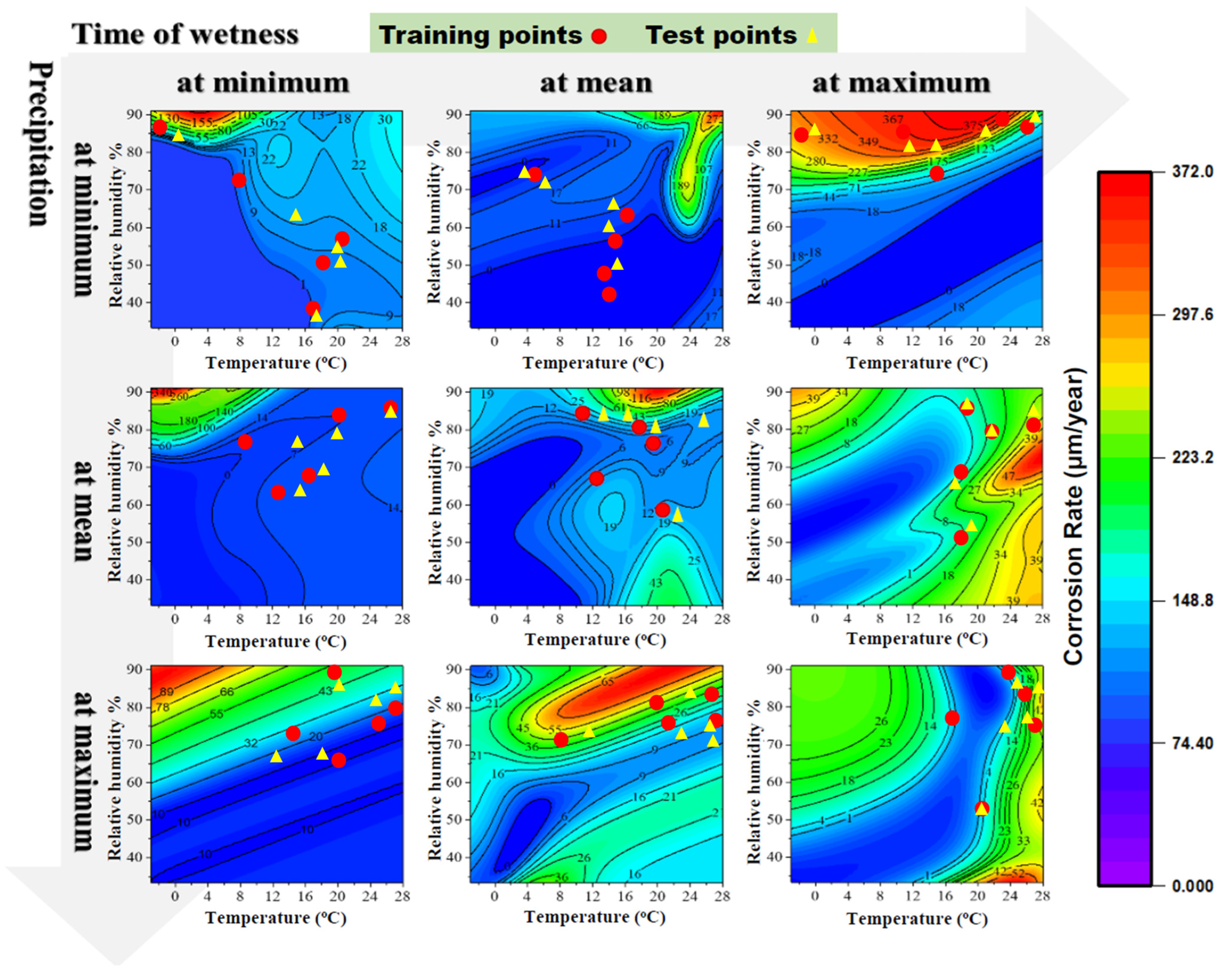
3.1. Heat Map

The heatmap (Figure 3) shows pairwise correlations between the environmental variables of temperature, RH, the TOW, precipitation, SO₂ concentration, chloride concentration, and the corrosion rate. This analysis was used to identify the initial relationships between these variables, thereby guiding the selection of the input features for the ANN model. The correlation analysis highlighted that the chloride concentration had the strongest positive correlation with the corrosion rate (~0.602), emphasizing its significant role in corrosion. RH (~0.711) and the TOW (~0.454) also showed strong positive correlations, indicating that increased humidity and prolonged wetness contribute to corrosion through electrochemical reactions. Precipitation correlated moderately with the TOW (~0.436) and temperature (~0.440), suggesting that wetter and warmer conditions may influence precipitate formation, which could facilitate corrosion. Temperature had weaker correlations with other variables and indirectly influenced corrosion by affecting the TOW. The SO₂ concentration showed a moderate correlation with the corrosion rate (~0.380), but its role in corrosion was less significant than that of chloride.

The very weak correlation between SO₂ concentration and RH (~0.026) suggests that humidity does not notably affect SO₂’s influence on corrosion. The heatmap provides preliminary insights into the most important environmental factors, such as chloride concentration, RH, and the TOW, which were selected as features for training the ANN model. These correlations guided the model’s input direction, ensuring that the most influential variables were included in the analysis.

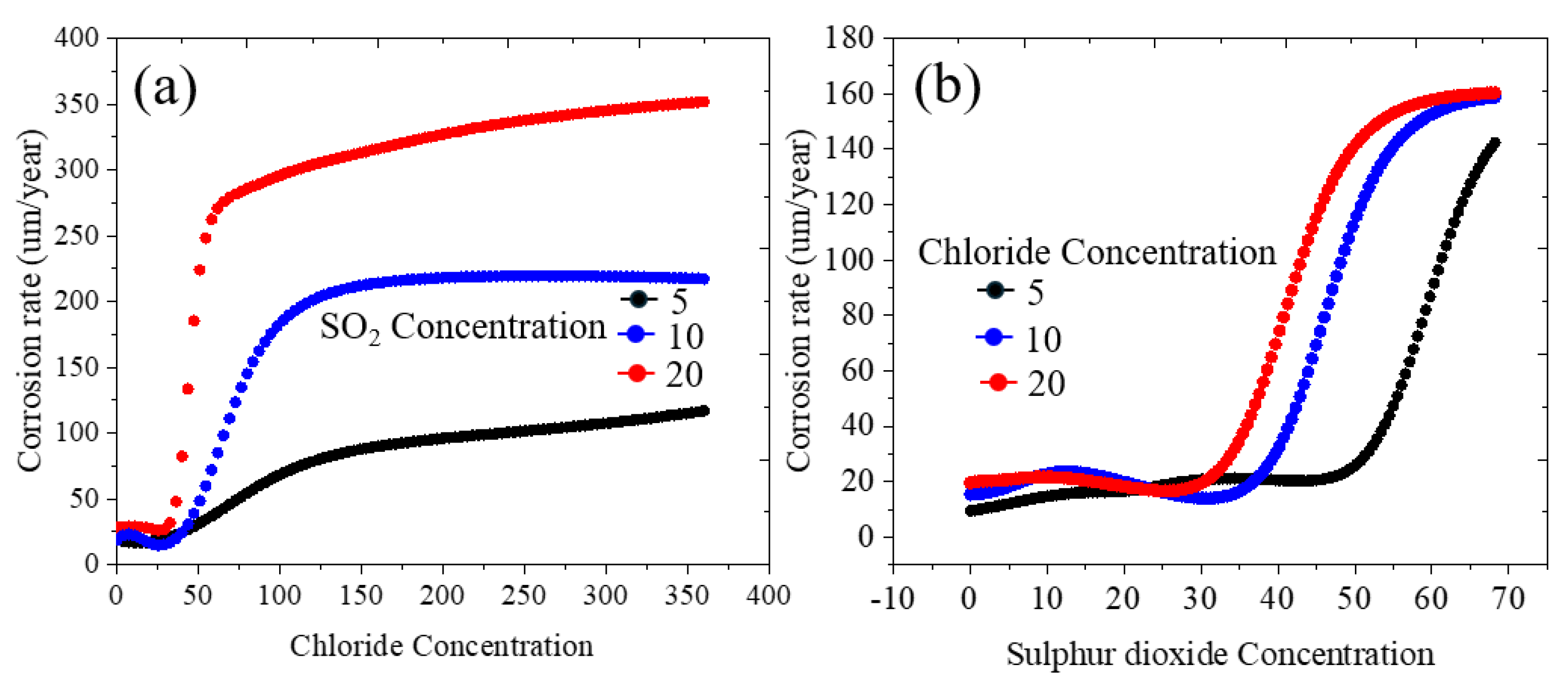
3.2. Predicted Corrosion Rate of Carbon Steel at Various Atmospheric Conditions

Figure 4 illustrates the predicted corrosion rate of carbon steel as a function of temperature (0–28.2 °C) and RH (33.3–91.1%) at varying wetness and precipitation times. For this analysis, SO₂ and chloride concentrations were held constant at their minimum values. The data revealed that, under minimum atmospheric conditions, a maximum corrosion rate of 155 μm/year occurs in regions with low temperatures (<8 °C) and high humidity (≈90%). This underscores the critical role of humidity in accelerating corrosion even at lower temperatures. When the TOW was at its minimum (0.003) and precipitation increased to its mean value (1093.42 mm), the corrosion rate increased to ~340 μm/year, likely due to increased surface moisture facilitating electrochemical reactions. Interestingly, when the precipitation was further increased to its maximum value (4656 mm), the corrosion rate decreased to ~89 μm/year, possibly because of a washing-off effect, where excessive rainfall removes accumulated corrosive agents from metal surfaces. To improve the interpretability of the model output, the training and test data points were overlaid on the representative central plot in Figure 4 (corresponding to the mean values of precipitation and TOW). These corrosion regions are supported by training data points (red circles), and yellow triangles represent test data distributed in plots, confirming that the observed nonlinear trends in the contour plot stem from the data itself rather than from model overfitting, thus reinforcing the predictive reliability of the ANN model.

This counterintuitive reduction in corrosion rate at extremely high precipitation levels can be explained by several mechanisms. First, continuous heavy rainfall can create a washing effect that removes accumulated corrosive agents from the metal surface, effectively cleansing the exposed sites [28]. Second, high volumes of precipitation can dilute the concentration of aggressive ions, such as chlorides and sulfates, in the moisture film on the metal surface, reducing their corrosive impact. Third, in areas with extremely high precipitation, frequent renewal of the electrolyte layer may prevent the buildup of corrosion products, which would otherwise accelerate localized corrosion through autocatalytic processes [29]. Additionally, at the minimum precipitation level (13 mm) and mean TOW (0.4785), the maximum corrosion rate (272 μm/year) was observed in regions with high temperatures (28 °C) and high humidity (90%). Increasing the TOW further increased the corrosion rate to a maximum of 375 μm/year and broadened the high-corrosion region. This suggests that extended exposure to moisture significantly accelerates corrosion, which is likely due to prolonged electrochemical reactions. Overall, the highest corrosion rates for carbon steel, exceeding 375 μm/year, occurred under the conditions of high temperature, high RH, high TOW, and low precipitation. These findings highlight the complex interplay between atmospheric conditions and their cumulative effects on corrosion rates. Understanding these interactions is crucial for predicting corrosion behavior in various environments and can guide maintenance strategies. For instance, areas with high humidity and temperature but low precipitation may require more frequent maintenance. In contrast, regions with high precipitation may benefit from the natural cleaning effect, reducing the need for intervention. Figure 3 provides a visual representation of these interactions, and additional insights into the model’s performance and visualization features are available in Supplementary Figures S1–S6. Supplementary Figure S7 provides a comprehensive validation analysis to check model reliability and data coverage. The data distribution (Figure S7a) demonstrates that training data exist throughout the temperature–humidity space, including in high-humidity regions where elevated corrosion rates are predicted. The model achieved excellent predictive accuracy (R² = 0.998, Figure S7b), with a consistent error distribution across all corrosion rate ranges (Figure S7c). Data density analysis (Figure S7d) confirmed adequate coverage in all environmental regimes, ensuring that the predictions represent interpolations rather than extrapolations.

Figure 5 illustrates the effect of the chloride and SO₂ concentrations on the corrosion rate of carbon steel. At this temperature, the relative humidity, time of wetness, and precipitation were maintained at their minimum values while varying the chloride and SO₂ concentrations. At a sulfate concentration of 5, an increase in the chloride concentration from 0 to 50 resulted in a relatively stable corrosion rate. However, a rapid increase in the corrosion rate was observed as the chloride concentration increased from 50 to approximately 100 mg/L, after which the rate continued at an almost constant level. A further increase in the sulfate concentration from 10 to 20 exhibited a similar trend, with an even higher overall corrosion rate compared to the previous condition. These findings indicate that a higher sulfate content exacerbates the corrosion rate, which is consistent with previous experimental observations [30] on the detrimental effect of chloride on the corrosion resistance.

We also predicted the effect of SO₂ concentration while keeping the chloride concentration constant, as shown in Figure 5b. At a fixed chloride concentration of 5, the corrosion rate remained nearly constant up to a SO₂ concentration of approximately 50. However, beyond this point, as the SO₂ concentration increased to 70, a significant increase in the corrosion rate was observed, followed by stabilization. A similar trend was noted for higher chloride concentrations of 10 and 20 with increasing SO₂ levels, leading to a further increase in the corrosion rate. It is worth mentioning that the adverse effect of rising SO₂ and chloride concentrations on corrosion resistance aligns well with previously reported experimental findings [31]. The ANN model accurately predicted the corrosion rate under varying conditions by keeping either the chloride or SO₂ concentration constant. This analysis offers valuable insights for managing corrosion in industrial and environmental settings where chloride and sulfur dioxide levels can fluctuate significantly.

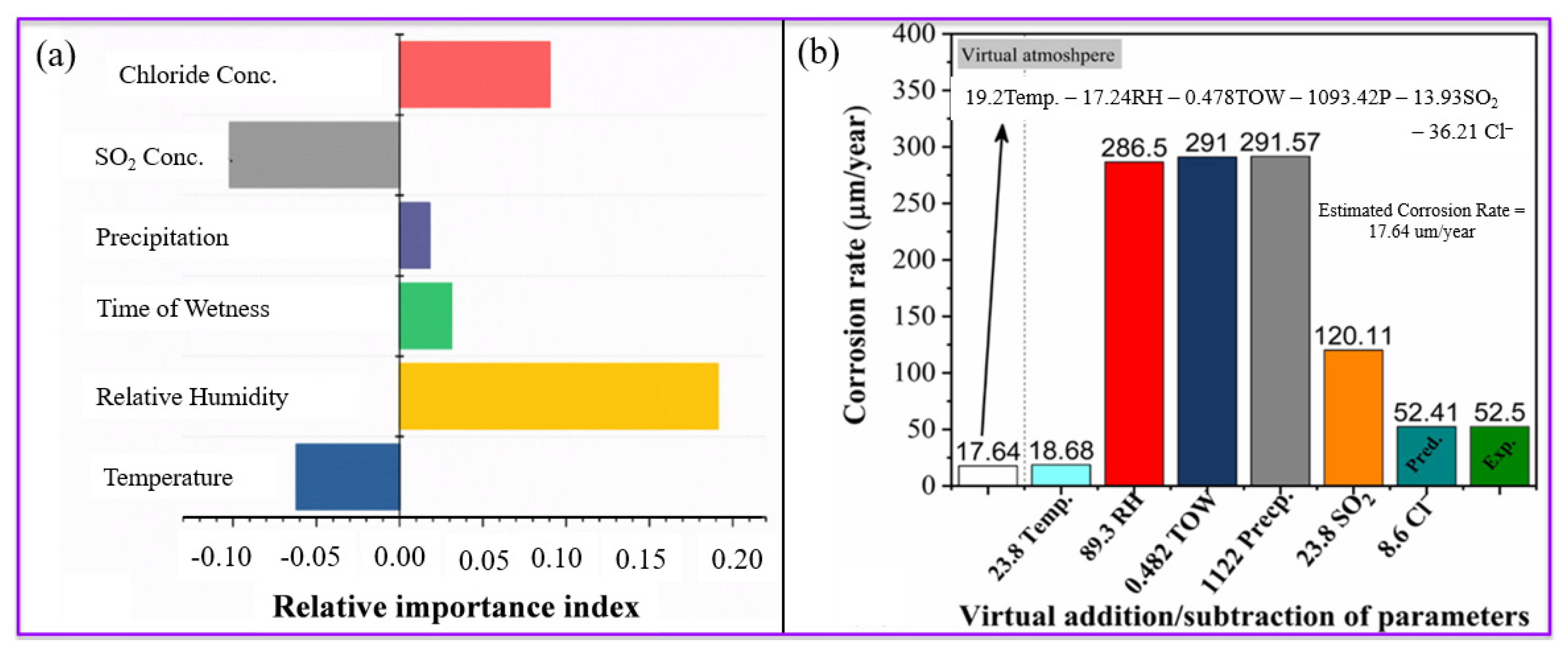
3.3. Qualitative and Quantitative Estimation of Corrosion Rate

The effects of atmospheric conditions on the corrosion rate of carbon steel were assessed using qualitative and quantitative methods. For the qualitative analysis, we employed a method known as the “index of relative importance”, which gauges the impact of various atmospheric factors. Figure 6a,b shows this analysis for dataset #15, revealing that RH, chloride concentration, the TOW, and precipitation positively affect the corrosion rate, with their influence decreasing in that order. In contrast, temperature and SO₂ concentrations had minimal effects. In the quantitative analysis, the corrosion rate was estimated under specific atmospheric conditions (dataset #15) using average values: 19.2 °C temperature, 17.24% RH, 0.478 fractions of year TOW, 1093.42 mm of precipitation, 13.93 mg/m².d of SO₂, and 36.21 mg/m².d of chloride concentration. The estimated corrosion rates for these conditions were 17.64 μm/year. Increasing the temperatures from 19.2 °C to 23.8 °C slightly increased the corrosion rate to 18.68 μm/year. Increasing RH from 17.24% to 89.3% significantly increased the rate to 286.5 μm/year, whereas further minor increases in the TOW and precipitation had negligible effects [30,31]. When the SO₂ concentration increased from 13.93 to 23.8 mg/m².d, it reduced the corrosion rate from 291.57 to 120.11 μm/year. Reducing the chloride concentration from 36.21 to 8.6 mg/m²·d further lowered the rate to 52.41 μm/year, which closely aligns with the experimentally measured value of 52.5 μm/year. These findings highlight the complex interactions among atmospheric conditions that affect corrosion rates.

The increase in corrosion rate with increasing RH and the significant effect of SO₂ at higher chloride levels reflect the intricate chemical and electrochemical processes involved. The close match between the estimated and experimental corrosion rates confirmed the accuracy of the proposed methods for predicting corrosion under varying atmospheric conditions. Furthermore, the importance of capturing microstructural effects on surface degradation has been demonstrated in other studies as well, such as in the work by Krbaťa et al. [32], who analyzed how thermal–mechanical deformation influences surface stability, wear resistance, and tribological performance in weld-modified steels under complex stress states. Overall, this analysis is crucial for developing corrosion-resistant materials and implementing maintenance strategies in environments with varying corrosive agents, thereby providing valuable insights for real-world applications.

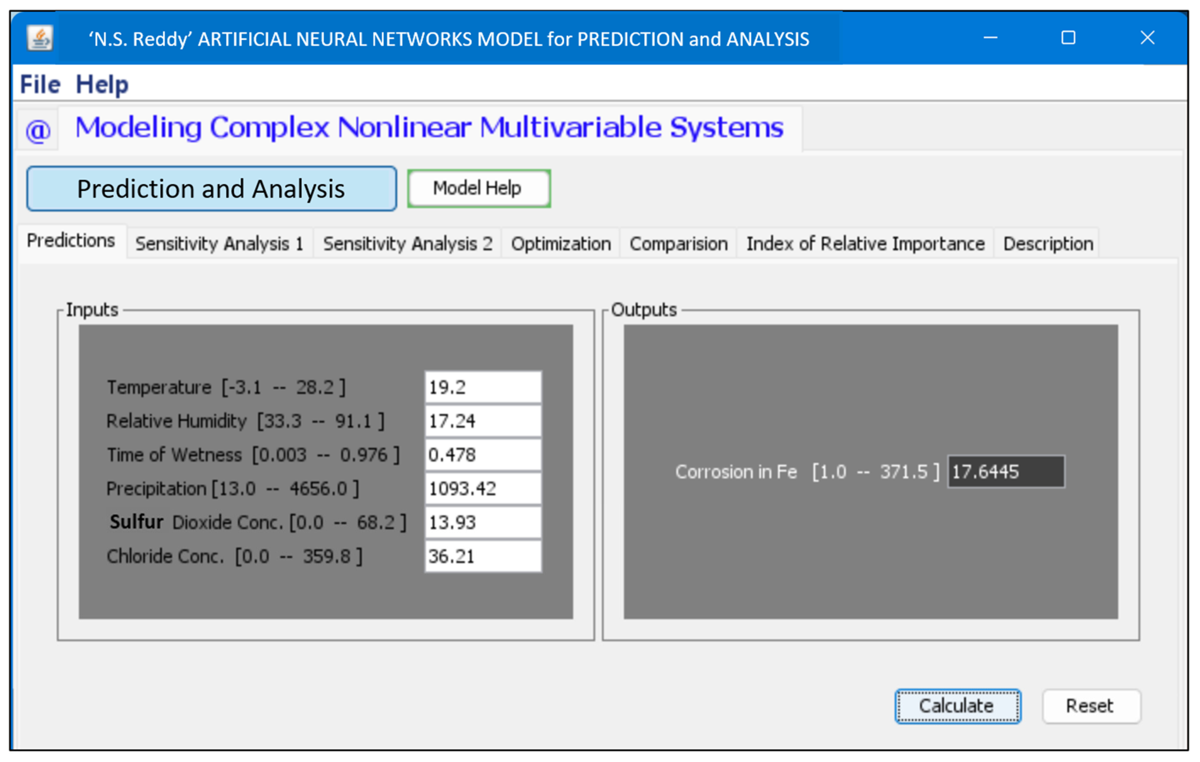
3.4. GUI for Corrosion Rate Prediction Using ANN

The ANN model was trained using the C program, and the GUI was developed using Java version 1.4, to enable cross-platform compatibility and efficient deployment. As shown in Figure 7, the GUI enables the accurate prediction of corrosion rates for infinite combinations of six input parameters: temperature, RH, the TOW, precipitation, SO₂ concentration, and chloride concentration.

The developed GUI enables users to predict corrosion rates with a single click, allowing the efficient exploration of various environmental conditions. It also supports sensitivity analysis to evaluate the influence of individual variables and their interactions, offering valuable insights into the complex nonlinear relationships affecting the corrosion behavior of carbon steels. This tool is particularly useful for optimizing service conditions and guiding material selection, thereby reducing the time and cost typically associated with experimental testing. The GUI and its source code can be provided upon request. Basic training and user support will also be offered to facilitate the broader use of the tool within the research community.

3.5. Limitations and Future Work

Although highly accurate, the ANN model is limited by its training data range, exclusion of potential synergistic effects from unmeasured pollutants, and a lack of time-dependent corrosion progression modeling. Future work should be expanded to include additional atmospheric variables, time-dependent behavior, and hybrid mechanistic-data-driven approaches. Extending the model to other structural materials and integrating them with IoT sensors for real-time monitoring represents promising development paths.

4. Conclusions

The major conclusions of this study are as follows:

• The developed ANN model showed excellent accuracy in predicting the corrosion rate of carbon steels with an R² of 97.2% for the training dataset and 95.6% for the testing dataset, demonstrating its effectiveness in capturing the complex relationships between atmospheric variables and corrosion rates.
• Among the atmospheric variables evaluated, relative humidity (RH) was found to have the most significant impact on corrosion rates, surpassing the influence of temperature and sulfur dioxide (SO₂) concentration.
• A graphical user interface (GUI) is provided, which offers an interactive and user-friendly platform for visualizing the effects of infinite combinations of various atmospheric parameters. With a GUI, one can easily predict the effect of a single variable, or the combined effect of two variables, can see the trend of increasing or decreasing the corrosion rate with a particular variable, and can also see the sensitivity analysis without prior knowledge of the programming.
• The model provides practical benefits in several key scenarios: (a) enabling condition-based maintenance for coastal infrastructure subject to variable corrosion risks, (b) optimizing inspection schedules for industrial facilities under changing climate conditions, (c) improving protective coating application timing for transportation infrastructure such as bridges and railways, and (d) helping utility companies prioritize maintenance resources across geographically distributed assets based on location-specific corrosion risk profiles.

References

1. Zhi, Y.; Jin, Z.; Lu, L.; Yang, T.; Zhou, D.; Pei, Z.; Wu, D.; Fu, D.; Zhang, D.; Li, X. Improving atmospheric corrosion prediction through key environmental factor identification by random forest-based model. Corros. Sci. 2021, 178, 109084. [Google Scholar] [CrossRef]
2. Pei, Z.; Zhang, D.; Zhi, Y.; Yang, T.; Jin, L.; Fu, D.; Cheng, X.; Terryn, H.A.; Mol, J.M.C.; Li, X. Towards understanding and prediction of atmospheric corrosion of an Fe/Cu corrosion sensor via machine learning. Corros. Sci. 2020, 170, 108697. [Google Scholar] [CrossRef]
3. Schweitzer, P.A. Atmospheric Degradation and Corrosion Control; CRC Press: Boca Raton, FL, USA, 1999. [Google Scholar]
4. Chico, B.; De la Fuente, D.; Díaz, I.; Simancas, J.; Morcillo, M. Annual atmospheric corrosion of carbon steel worldwide. An integration of ISOCORRAG, ICP/UNECE and MICAT databases. Materials 2017, 10, 601. [Google Scholar] [CrossRef] [PubMed]
5. Ishtiaq, M.; Inam, A.; Tiwari, S.; Seol, J.B. Microstructural, mechanical, and electrochemical analysis of carbon doped AISI carbon steels. Appl. Microsc. 2022, 52, 10. [Google Scholar] [CrossRef]
6. LeBozec, N.; Jonsson, M.; Thierry, D. Atmospheric corrosion of magnesium alloys: Influence of temperature, relative humidity, and chloride deposition. Corrosion 2004, 60, 356–361. [Google Scholar] [CrossRef]
7. Wang, X.; Li, X.; Tian, X. Influence of temperature and relative humidity on the atmospheric corrosion of zinc in field exposures and laboratory environments by atmospheric corrosion monitor. Int. J. Electrochem. Sci. 2015, 10, 8361–8373. [Google Scholar] [CrossRef]
8. Cai, Y.; Zhao, Y.; Ma, X.; Zhou, K.; Chen, Y. Influence of environmental factors on atmospheric corrosion in dynamic environment. Corros. Sci. 2018, 137, 163–175. [Google Scholar] [CrossRef]
9. Mansfeld, F. Atmospheric corrosion rates, time-of-wetness and relative humidity. Mater. Corros. 1979, 30, 38–42. [Google Scholar] [CrossRef]
10. Jain, S.; Jain, R.; Wagri, N.K.; Sikarwar, A.S.; Khaire, S.J.; Dewangan, S.K.; Jeon, Y.; Ahn, B. Reducing experimental dependency: Machine-learning-based prediction of Co effects on the mechanical properties of AlCrFeNiCox high-entropy alloys. Mater. Today Commun. 2025, 44, 112055. [Google Scholar] [CrossRef]
11. Cho, M.; Gim, J.; Kim, J.H.; Kang, S. Development of an Artificial Neural Network Model to Predict the Tensile Strength of Friction Stir Welding of Dissimilar Materials Using Cryogenic Processes. Appl. Sci. 2024, 14, 9309. [Google Scholar] [CrossRef]
12. Kamrunnahar, M.; Urquidi-Macdonald, M. Prediction of corrosion behavior using neural network as a data mining tool. Corros. Sci. 2010, 52, 669–677. [Google Scholar] [CrossRef]
13. Zadeh Shirazi, A.; Mohammadi, Z. A hybrid intelligent model combining ANN and imperialist competitive algorithm for prediction of corrosion rate in 3C steel under seawater environment. Neural Comput. Appl. 2017, 28, 3455–3464. [Google Scholar] [CrossRef]
14. Birbilis, N.; Cavanaugh, M.K.; Sudholz, A.D.; Zhu, S.M.; Easton, M.A.; Gibson, M.A. A combined neural network and mechanistic approach for the prediction of corrosion rate and yield strength of magnesium-rare earth alloys. Corros. Sci. 2011, 53, 168–176. [Google Scholar] [CrossRef]
15. Wen, Y.F.; Cai, C.Z.; Liu, X.H.; Pei, J.F.; Zhu, X.J.; Xiao, T.T. Corrosion rate prediction of 3C steel under different seawater environment by using support vector regression. Corros. Sci. 2009, 51, 349–355. [Google Scholar] [CrossRef]
16. Shi, J.; Wang, J.; Macdonald, D.D. Prediction of primary water stress corrosion crack growth rates in Alloy 600 using artificial neural networks. Corros. Sci. 2015, 92, 217–227. [Google Scholar] [CrossRef]
17. Pintos, S.; Queipo, N.V.; Troconis de Rincón, O.; Rincón, A.; Morcillo, M. Artificial neural network modeling of atmospheric corrosion in the MICAT project. Corros. Sci. 2000, 42, 35–52. [Google Scholar] [CrossRef]
18. Lee, S.; Narayana, P.L.; Seok, B.W.; Panigrahi, B.B.; Lim, S.-G.; Reddy, N.S. Quantitative estimation of corrosion rate in 3C steels under seawater environment. J. Mater. Res. Technol. 2021, 11, 681–686. [Google Scholar] [CrossRef]
19. Chen, B.; Ge, B.; Zhang, X.; Yang, D.; Yang, P.; Lu, W.; Min, J.; Ming, P.; Zhang, C. Role of oxide layer on corrosion resistance and surface conductivity of titanium bipolar plates for proton exchange membrane fuel cell. J. Power Sources 2024, 624, 235637. [Google Scholar] [CrossRef]
20. Kordas, G. Corrosion Barrier Coatings: Progress and Perspectives of the Chemical Route. Corros. Mater. Degrad. 2022, 3, 376–413. [Google Scholar] [CrossRef]
21. Pilch, O.; Faltejsek, P.; Hurby, V.; Krbata, M. The Corrosion Resistance of Turbocharger Stator after Plasma Nitriding Process. Manuf. Technol. 2017, 17, 360–364. [Google Scholar] [CrossRef]
22. Yadav, A.; Panjikar, S.; Raman, R.K.S. Graphene-Based Impregnation into Polymeric Coating for Corrosion Resistance. Nanomaterials 2025, 15, 486. [Google Scholar] [CrossRef]
23. Song, Z.; Song, H.; Liu, J.; Liu, H. Tuning heterogeneous microstructure and improving mechanical properties of twin-roll strip cast low carbon steels by on-line heat treatments. J. Mater. Res. Technol. 2024, 30, 5894–5904. [Google Scholar] [CrossRef]
24. ISO 9223; Corrosion of Metals and Alloys—Corrosivity of Atmospheres—Classification, Determination and Estimation. International Organization for Standardization: Geneva, Switzerland, 2012.
25. ASTM G92; Standard Practice for Characterization of Atmospheric Test Sites. ASTM International: West Conshohocken, PA, USA, 2020.
26. Reddy, N.S.; Krishnaiah, J.; Hong, S.-G.; Lee, J.S. Modeling medium carbon steels by using artificial neural networks. Mater. Sci. Eng. A 2009, 508, 93–105. [Google Scholar] [CrossRef]
27. Zhang, X.; He, W.; Odnevall Wallinder, I.; Pan, J.; Leygraf, C. Determination of instantaneous corrosion rates and runoff rates of copper from naturally patinated copper during continuous rain events. Corros. Sci. 2002, 44, 2131–2151. [Google Scholar] [CrossRef]
28. Cole, I.S.; Paterson, D.A.; Ganther, W.D. Holistic model for atmospheric corrosion Part 1—Theoretical framework for production, transportation and deposition of marine salts. Corros. Eng. Sci. Technol. 2003, 38, 129–134. [Google Scholar] [CrossRef]
29. Xue, F.; Wei, X.; Dong, J.; Wang, C.; Ke, W. Effect of chloride ion on corrosion behavior of low carbon steel in 0.1 M NaHCO3 solution with different dissolved oxygen concentrations. J. Mater. Sci. Technol. 2019, 35, 596–603. [Google Scholar] [CrossRef]
30. Xiang, Y.; Wang, Z.; Xu, C.; Zhou, C.; Li, Z.; Ni, W. Impact of SO2 concentration on the corrosion rate of X70 steel and iron in water-saturated supercritical CO2 mixed with SO2. J. Supercrit. Fluids 2011, 58, 286–294. [Google Scholar] [CrossRef]
31. Pei, Z.; Cheng, X.; Yang, X.; Li, Q.; Xia, C.; Zhang, D.; Li, X. Understanding environmental impacts on initial atmospheric corrosion based on corrosion monitoring sensors. J. Mater. Sci. Technol. 2021, 64, 214–221. [Google Scholar] [CrossRef]
32. Krbata, M.; Ciger, R.; Kohutiar, M.; Sozańska, M.; Eckert, M.; Barenyi, I.; Kianicova, M.; Jus, M.; Beronská, N.; Mendala, B.; et al. Effect of Supercritical Bending on the Mechanical & Tribological Properties of Inconel 625 Welded Using the Cold Metal Transfer Method on a 16Mo3 Steel Pipe. Materials 2023, 16, 5014. [Google Scholar] [CrossRef]
Figure 1. Schematic representation of the ANN model architecture trained using the backpropagation algorithm.
Metals 15 00607 g001
Figure 2. (a) Variation in test data error as a function of iterations. (b) Experimental vs. predicted corrosion rate plot of 105 test datasets. (c) Comparison plot of experimental and predicted corrosion rates (um/year) for 25 test datasets.
Metals 15 00607 g002
Figure 3. Heatmap of correlation coefficients between environmental variables and corrosion rate.
Metals 15 00607 g003
Figure 4. Predicted corrosion rate of carbon steel as a function of temperature and relative humidity at the minimum, mean, and maximum values of wetness and precipitation, respectively. The other two atmospheric conditions (SO2 and Cl) were maintained to a minimum.
Metals 15 00607 g004
Figure 5. Predicted corrosion rate of carbon steel as a function of (a) chloride and (b) sulfur dioxide concentrations. The other variables are kept at a minimum.
Metals 15 00607 g005
Figure 6. (a) Qualitative (relative importance index) and (b) quantitative influence of atmospheric conditions on the corrosion rate of carbon steel. The estimated behavior is for Dataset #15.
Metals 15 00607 g006
Figure 7. GUI for estimating the corrosion rate by manually entering atmospheric conditions. The developed ANN model features a user-friendly GUI designed to predict the corrosion rate of carbon steel.
Metals 15 00607 g007