Article

Residual Temperature Prediction in Selective Laser Melting by Deep Neural Networks

by
Nikolaos Papadimitriou
,
Emmanuel Stathatos
and
George-Christopher Vosniakos
*
Manufacturing Technology Laboratory, School of Mechanical Engineering, National Technical University of Athens, 15773 Athens, Greece
*
Author to whom correspondence should be addressed.
Metals 2025, 15(10), 1119; https://doi.org/10.3390/met15101119
Submission received: 4 September 2025 / Revised: 3 October 2025 / Accepted: 7 October 2025 / Published: 9 October 2025

Abstract

Selective laser melting (SLM) builds metal parts layer by layer by locally melting powder with a fine laser beam, generating complex, geometry-dependent temperature gradients that govern density, microstructure, defects, and residual stresses. Resolving these gradients with high-fidelity finite-element (FE) models is prohibitively slow because the temperature field must be evaluated at dense points along every scan track across multiple layers, while the laser spot is orders of magnitude smaller than typical layer dimensions. This study replaces FE analysis with a deep neural network that predicts the end-of-build temperature field orders of magnitude faster. A benchmark part containing characteristic shape features is introduced to supply diverse training cases, and a novel control-volume-based geometry-abstraction scheme encodes arbitrary workpiece shapes into compact, learnable descriptors. Thermal simulation data from the benchmark train the network, which then predicts the residual temperature field of an unseen, geometrically dissimilar part with a mean absolute error of ~10 K and a mean relative error of ~1% across 500–1300 K. The approach thus offers a rapid, accurate surrogate for FE simulations, enabling efficient temperature-driven optimization of SLM process parameters and part designs.

1. Introduction

1.1. Background and Motivation

The SLM process functions by sequentially depositing thin layers of metal powder on a powder bed using a roller and a powder delivery system, after which a laser selectively melts the powder, which then solidifies as a layer of the final part. The process repeats as the powder bed lowers to accommodate each new layer until the part is complete [1]. SLM can produce highly complex geometries, making it suitable, among many other uses, for aerospace components (e.g., fuel nozzles) [1] and for automotive applications [2]. This technology has shown immense development and is steadily being adopted for more and more use cases; however, it presents features that make it harder to model compared to other manufacturing processes.
Residual stress emergence, deformation, microstructure, and general mechanical properties of the part all stem from temperature evolution in time and space across the part. Therefore, prediction of full thermal history in time and space is ideally necessary in a coupled thermos-mechanical model.
Numerical FE models can yield accurate results, but their accuracy depends strongly on model fidelity. Fully resolving phenomena down to the powder-particle scale is computationally infeasible for regular-sized parts. Moreover, process effects such as volumetric shrinkage and evaporation are difficult to represent and further increase model complexity [3]. To address these limitations, abstraction methodologies use small-scale models to identify effective heat-input and material parameters that can be upscaled to part-level analyses [4,5,6]. This upscaling allows the part to be meshed at resolutions much coarser than the powder-particle scale while preserving the averaged thermal response. Consequently, current approaches mesh the part with elements that are large relative to the process microscale. Further reducing element size can improve fidelity but renders the simulations prohibitively time-consuming [7].

1.2. Prior Work

Qi et al. [8] argue that neural networks (NNs) can accelerate design decisions and the estimation of part properties in SLM without the heavy computational cost of traditional simulations. Feng et al. [9], for example, devised a method where a physics-informed neural network predicts the fatigue life of SLM-produced parts based on their defects. Demir et al. [10] used a descriptor for the SLM laser scan path to train a neural network to predict in situ and post-printing defects. Xing et al. [11] used computer vision and image processing to train a neural network that is able to recognize and classify melt tracks in order to determine optimal laser power and scan speed. A form of temperature prediction using neural networks was achieved by Gao et al. [12] using a backpropagating neural network to accurately determine molten pool temperature and processing quality, using laser power, scanning speed, and powder feeding rate as inputs.
Evidently, neural networks have been applied to process planning, quality control, and real-time monitoring [13], However, most existing models target localized phenomena—such as melt tracks, single layers, or melt-pool behavior—or serve as task-specific classifiers [11,12,14]. By contrast, learning-based surrogates that predict spatially resolved temperature and/or stress fields across the entire build—conditioned on both process parameters and part geometry, as a part-scale alternative to thermo-mechanical finite-element analysis—remain limited. Wu et al.’s review on the residual stress prediction highlights the predominance of finite-element methods, with little coverage of NN-based, part-scale models [15]. This gap motivates approaches that are geometry-aware and produce full-field predictions over the entire printed part.
To use a part’s shape as a network input, geometry must be abstracted into features suitable for learning. Belongie et al. [16] introduced “shape contexts”, which describe a 2D shape by sampling points on its contour and, for each point, constructing a log-polar histogram of the relative positions of all other sampled points, enabling both matching and localized shape description. Angrish et al. [17] proposed an algorithm where manufacturing parts are classified using an image conversion as input to a convolutional neural network along with metadata. This method, however, along with other general 3D shape descriptors, does not produce results that can be attributed to specific points of the part and thus cannot be used to predict a property of a part in a desired location. Bacciaglia et al. [18] reported the widespread use of voxelization, i.e., discretization of a part into six- sided elements, for use in geometry manipulation of SLM parts. Voxels indeed describe a part in great detail and also provide numerical data for isolated locations of a part, but do not by themselves encode discriminative neighborhood context for learning compact inputs. Addressing this, Wang et al. [19] derived features from the presence or absence of neighboring voxels to feed a network for semantic segmentation, illustrating how local voxel neighborhoods can yield informative per-voxel descriptors.

1.3. Research Gap, Aim, and Contributions

Despite progress in extracting geometry-derived descriptors and in applying neural networks within the SLM workflow, there remains a lack of a geometry-aware, part-scale surrogate that maps part geometry and process parameters to a spatially resolved temperature field for the entire build.
This paper addresses that gap through three contributions:
(i)
a benchmark part that concentrates representative geometric features to generate diverse training and evaluation cases,
(ii)
a geometry-abstraction algorithm that yields per-location descriptors via intersections between predefined control volumes (CVs) and the part, and
(iii)
a deep neural network trained on simulation-generated data to predict residual temperature at arbitrary locations, enabling full-field prediction far more efficiently than finite-element analysis.
Full-temperature field prediction in time and space, if it were computationally feasible and if suitable models connecting it to process parameters existed, would ideally enable prediction of mechanical properties and microstructure of the part and possibly lead to off-line optimization of process parameters before production, which would also ease the machine controller’s job. However, the value of predicting the residual temperature field at a single time snapshot, e.g., at the end of the printing job, should not be overlooked. This could provide hints for (a) process improvement in the next repetition of the same building job, (b) an assessment of the level of resulting residual stress and distortion in the part, and (c) prioritizing part inspection actions, concentrating on particular regions.
This paper is structured in the following way: Section 2 presents geometry representation and abstraction; Section 3 outlines the development of the neural network and explains the test scenarios; Section 4 presents results focusing on the baseline accuracy benchmarks, robustness to geometric changes, input significance studies, and scalability across multiple part sizes; and Section 5 provides a high-level discussion of the findings and their significance. Conclusions, current limitations, and possible future work are discussed in Section 6.

2. Part Shape Modeling

2.1. Benchmark Part Design

The benchmark design is driven by the goals of this study and by needs that extend beyond its immediate scope. Accordingly, it must support multiple use cases and provide meaningful data for each. The design requirements were:
  • Contain a variety of geometric features in order to provide varying data to train the neural network
  • Have a reasonable degree of asymmetry
  • Fit within a relatively small-sized bounding box
  • Allow for post-printing measurement
  • Provide material for mechanical testing
  • Minimize geometry below a 1 mm voxel resolution so that analysis remains computationally viable
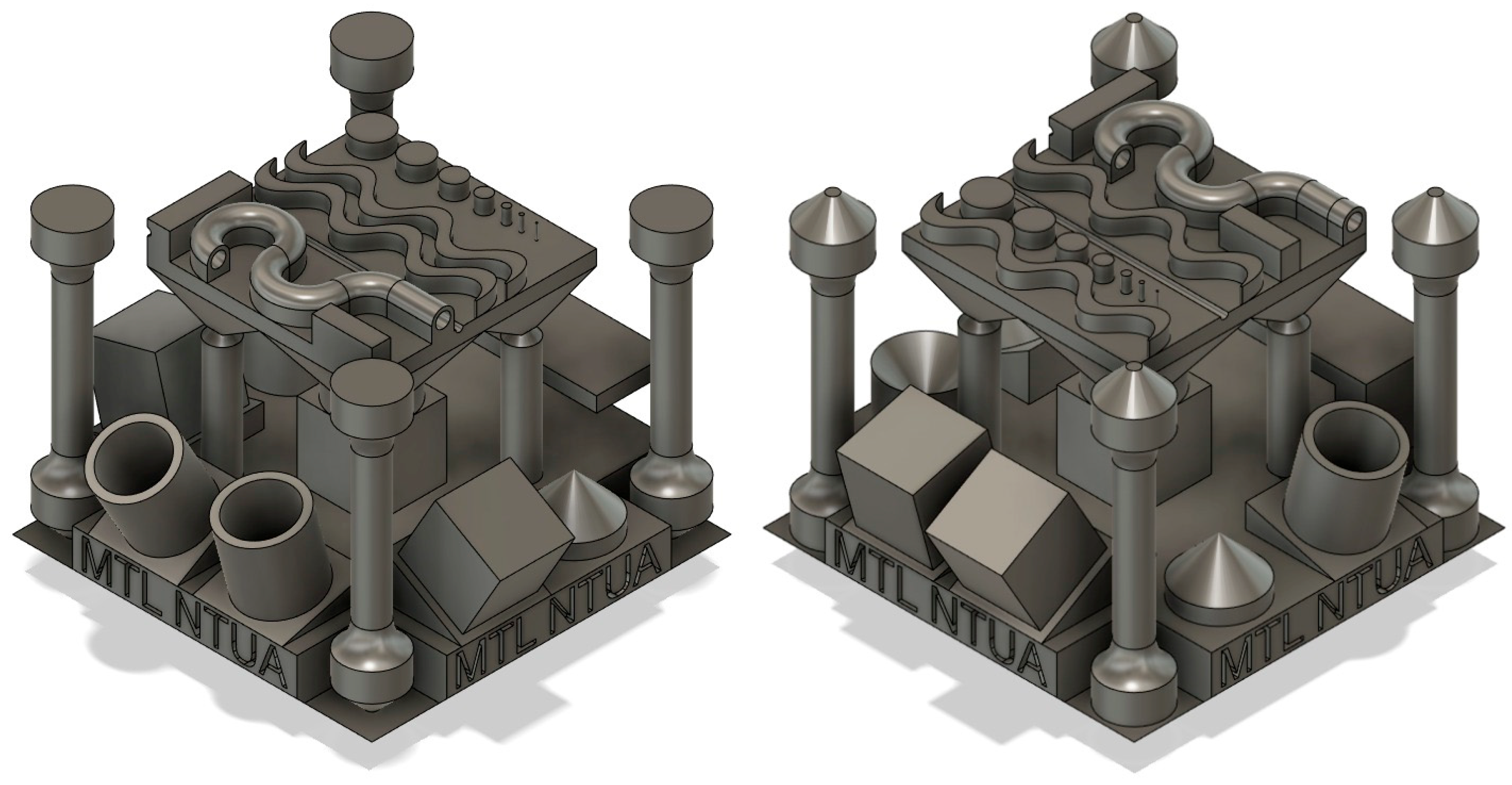
As existing research does not offer a benchmark part that satisfies these requirements, the part was created from scratch. During its design, scientific papers proposing parts for similar use cases were referenced to provide example geometries aligned with the above criteria. The resulting feature set includes sloped planes, cubes, and cylinders in order to evaluate geometric dimensioning and tolerancing (GD and T) of the printed part [20]; detachable chemical and mechanical testing parts, as well as overhangs and an internal channel [21]; and finally sharp pointed extrusions and cavities [22]. The finalized part, as shown in Figure 1, consolidates all the aforementioned design decisions in a format that fits inside a cubical bounding box with a 60 mm side length. FusionTM by AutodeskTM (Version v.2.0.19941) was used to create the CAD model.

2.2. Geometry Abstraction

In order to create an abstraction of the geometrical characteristics of a given CV, a simple formula was created.
D = V p a r t V c o n t r o l
here Vpart is the volume of the part which the CV intersects and Vcontrol is the volume of the CV. The resulting D (density) describes how densely the CV is filled with the part. A value of 1 signifies 100% of the CV intersects with the part with zero air gaps, while a value of 0 signifies it has no intersections with the part and is entirely composed of air.
In Figure 2, an example is shown using the benchmark part and a cubical volume with an 8 mm side length. The intersection of the two is highlighted. In this case, Vcontrol is easily calculated as 512 square millimeters, while the intersection of the CV and the part can be calculated with FusionTM as 105.702 square millimeters. The resulting D would then be equal to 0.206.
In practice, multiple CVs would be used in order to describe the geometry around a point. It is evident, however, that reducing the volume and increasing the count of the CVs would result in describing the part in increasing detail, eventually resulting in values that are either 0 or 1. This would be the same as creating a complete 3D voxel approximation of the part, which is not the level of abstraction that is pursued in this case. The goal is to describe part geometry using only a fraction of the values that would be used to recreate it with voxels while maintaining an appropriate value count for use as input for a deep neural network (DNN).

2.3. CV Positioning and Calculation

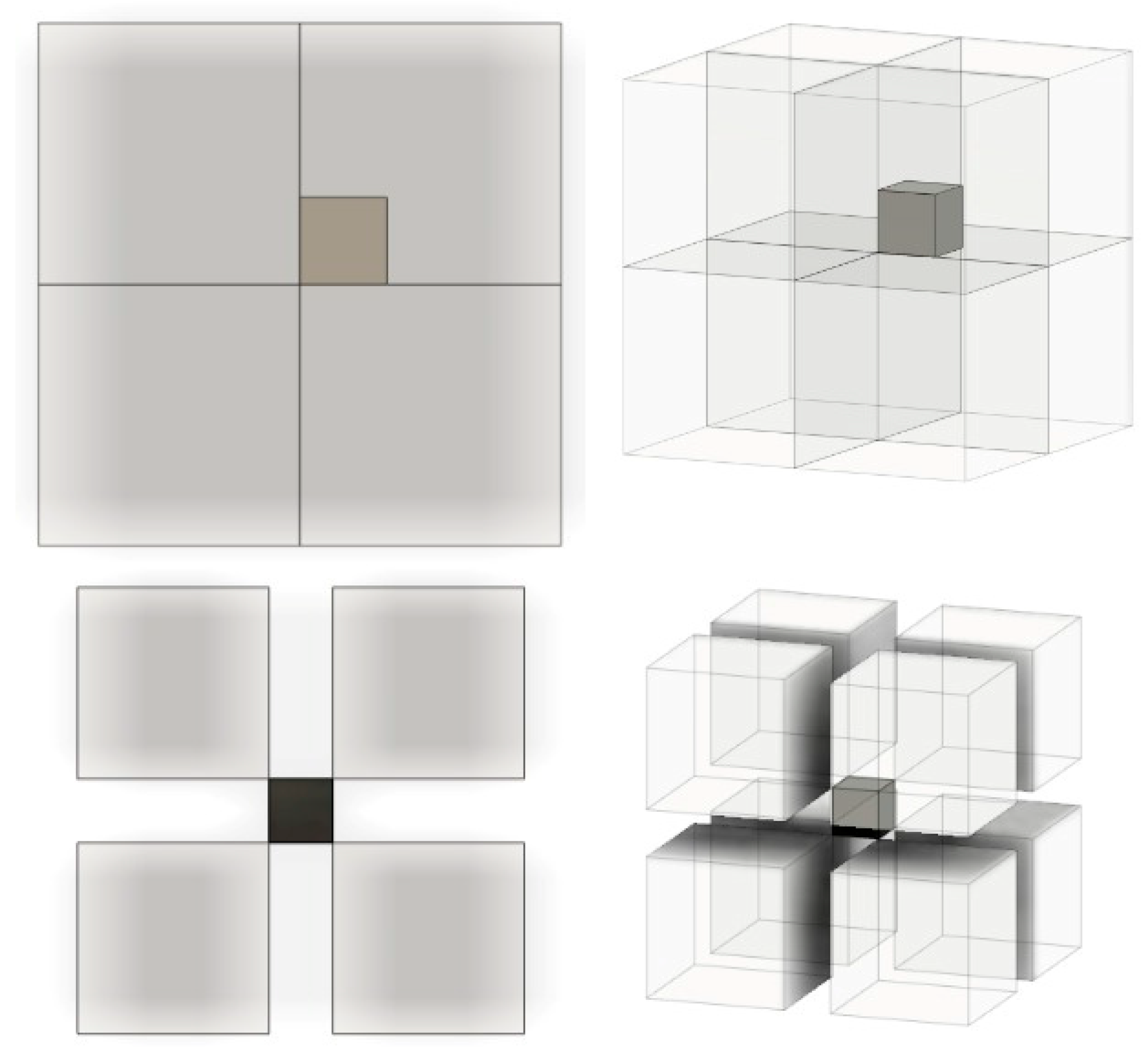
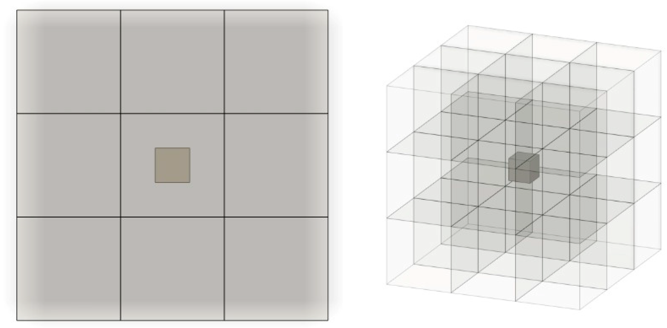
CVs were deployed at deterministic, repeatable offsets with respect to the voxel under investigation so that the DNN received consistent inputs across the entire dataset. Their size and count were governed by two scalar parameters, thereby permitting systematic parametric studies. Because the computational domain is discretized on a regular grid derived from the shape array, the edge length of each CV was expressed as an integer number of elements. Consequently, Vcontrol denotes the total number of grid elements enclosed by a CV, whereas Vpart represents the subset of those elements that possess a value of 1 in the shape array. For geometric symmetry and to eliminate orientation bias, all CVs were defined as cubes of identical size. Three candidate placement strategies were evaluated, subject to the constraint that the framework remain scalable via simple changes to a few input variables. When an even number of CVs is employed, the central voxel either lacks a unique enclosing CV or is separated from neighboring CVs by void regions, as illustrated in Figure 3 (element size = 1 mm; CV edge length = 3 mm). Both scenarios lead to directionally skewed sampling or data gaps. In contrast, selecting an odd number of CVs resolves this issue: the voxel under examination can be positioned at the geometric center of the central CV (Figure 4, identical dimensions). This requirement also imposes that the CV edge length itself be an odd number of grid elements; otherwise, no true center exists within the CV for voxel alignment. The parameters used in the code to determine the size and number of the CVs are as such.
  • Box radius: The distance from the center element to the side of the cube measured in elements (would be equal to 1 in Figure 4)
  • Box grid size: The cube root of the total amount of CVs, or the number of CVs along an edge of the total checked volume (would be equal to 3 in Figure 4)

2.4. Code Implementation

In MATLABTM (Version R2024b), the control-volume “density” is computed by querying a binary, integer-indexed 3D array constructed from the AltairTM print3D (Version 2022) element centroids. Initial tests used cube-shaped CVs for ease of implementation. The approach relies on the fixed element size in the simulation mesh, which implies constant orthogonal spacing between element centroids. The following steps were followed in order to transform the initial data into a format with which the CV calculation can take place with increased efficiency:
  • Subtraction of the minimum coordinate value per axis in order to make all coordinates positive, while maintaining identical relative distances and creating a zero point in the process to serve as an origin point
  • Division of all coordinate values by element size, resulting in integers
  • Addition of a set integer to all coordinates in order to create an offset from the origin point
  • Creation of a 3D zero array with each dimension’s size equal to the sum of the size of the part along that dimension and the offset integer multiplied by 2
  • Population of the array by setting the values whose array index coincides with a coordinate set from the transformed initial data to 1
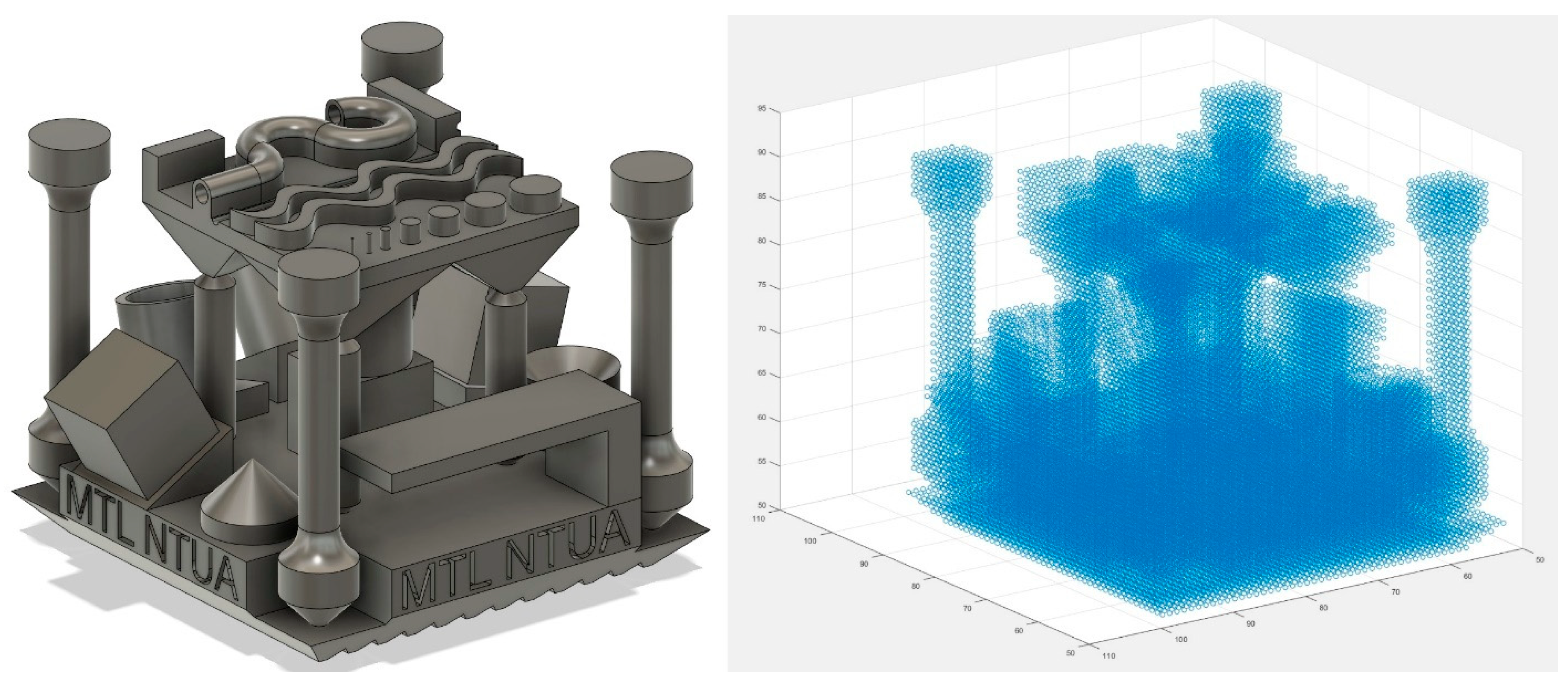
This array constitutes a 3D “shape array” (see Figure 5) that mirrors the part’s occupancy. It enables direct membership tests for any grid location—both inside the part and in surrounding air—eliminating repeated searches through the original coordinate table. This massively speeds up the computation time needed to extract all the data required to determine the resulting values from the CV analysis. For the full part with a large CV, runtime was reduced from hundreds of hours (table queries) to roughly one minute (indexed lookups). A range-query approach based on k-d trees was also rejected [23] because Euclidean-distance neighborhoods are spherical, and spheres cannot tile 3D space without overlap or gaps. Overlap would feed multiple inputs of the neural network with data from the same region (duplicated information), whereas gaps would omit segments of the part geometry.

3. Deep Neural Network Development

3.1. DNN Configuration

The neural network developed has 28 inputs, 27 from CV data and the last one representing element height, and one output (temperature). The height feature is defined as the distance from the element centroid to the top surface of the part (in meters). Because layers are deposited sequentially, a greater distance from the top correlates with longer elapsed time since direct laser exposure, which helps the model capture cooling history. Additionally, the CV values are processed with the MATLABTM function ‘mapminmax’, in order to avoid inputting values of 0 in the neural network. A total of 20% of the data is reserved as a hold-out validation set and is never used for training. After training, predictions on this set are compared with ground-truth temperatures using mean squared error (MSE), mean relative error (MRE), and mean absolute error (MAE). Training is accelerated using MATLABTM’s Parallel Computing Toolbox, which enables GPU cores for computation. The algorithm chosen for training was the scaled conjugate gradient backpropagation (trainscg in MATLABTM) algorithm and the transfer function is the hyperbolic tangent sigmoid function (tansig in MATLAB).

3.2. Dataset Generation from Process Simulations

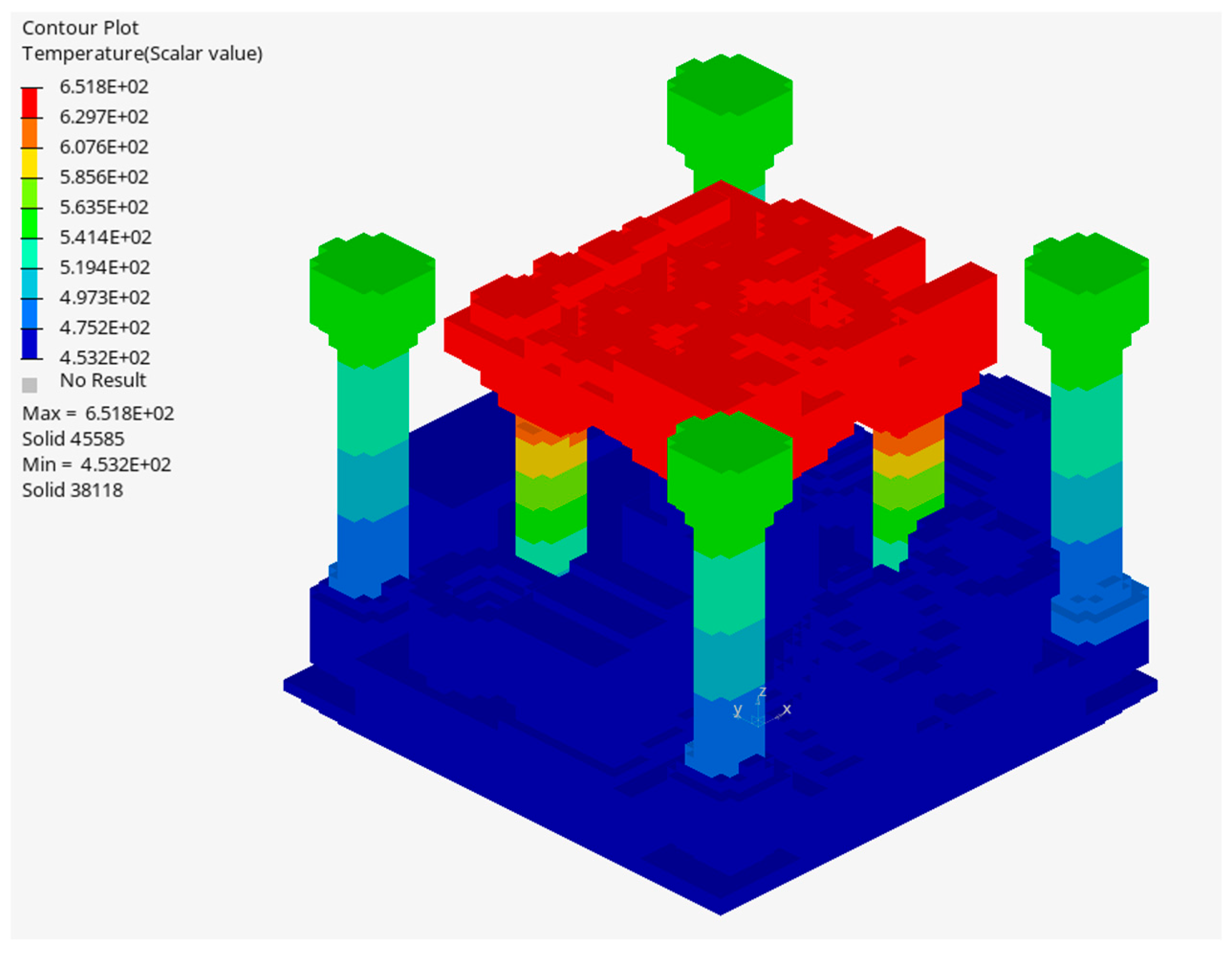
In order to obtain training data, AltairTM print3D, which is part of the AltairTM Inspire software suite, was used. More specifically, version 2022 was used, as newer versions do not output results of thermal nature. All settings were left at default except where specified in this article, and the material used for the simulation was 316L steel with a 1 mm element size. Importantly, the cooldown time was set to 10 secs, with all the extracted data pertaining to that time. This timeframe was chosen since it is not long enough for the temperature to equalize within the part, which would make the temperature gradient unusable for determining high temperature retention areas. These parameters along with additional ones are shown in Table 1. A characteristic snapshot of residual temperature fields is shown in Figure 6.
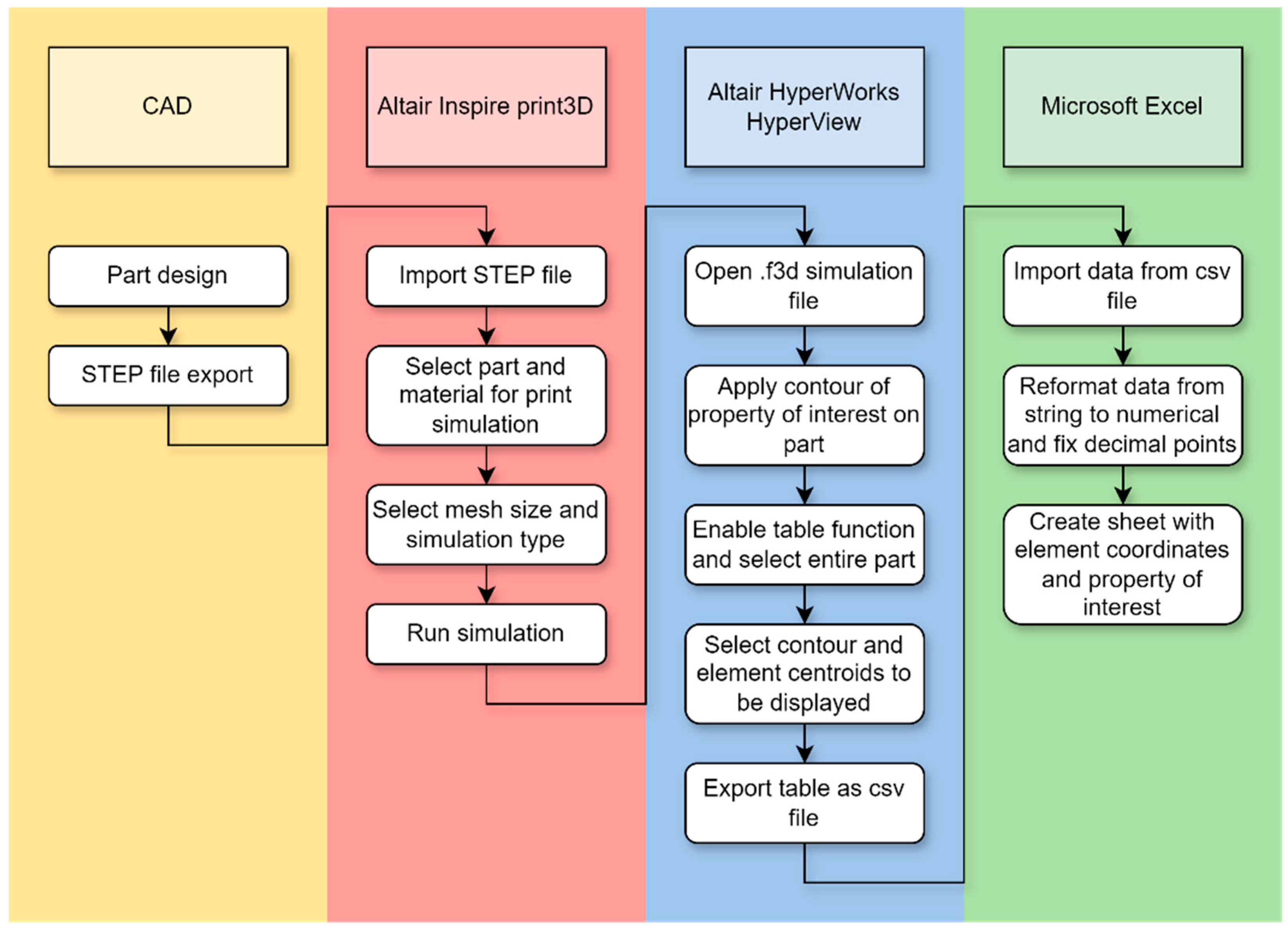
It is worth noting that the software does not export data in comma-separated values (CSV) format, only finalized STL models. For this reason, AltairTM HyperView (Version 2024) is used, which is part of the AltairTM HyperWorks. Its capabilities include extracting data from analysis performed with print3D, which was used to obtain the data needed for training the neural network. The data chosen for extraction included the ID of the element, its centroid, as well as its temperature. After parsing and cleaning, the final dataset retained temperature together with the Cartesian coordinates of each element centroid and was saved in .xlsx format. The workflow for the data extraction is also shown in Figure 7.

3.3. Testing Scenarios

Initially, a basic test for the model is designed, where data only from the base benchmark part is used for training and validation, resulting in a dataset with 44,738 rows, numbering equal to the voxel count of the part. This is to verify the basic functions of the model and to establish correlations between the selected inputs and outputs. The DNN has five hidden layers with [27,18,27,27,18] neurons, respectively, with box radius set to two and box grid size set to three. These CV parameters were selected after considering the size of the part as well as the size of its solid sections, with a general rule that CVs should intersect with the feature of the part that the currently examined element belongs to and at least one neighboring feature. Through preliminary analysis, higher and lower values in either parameter provided worse results. Actually, deviating from these values yields extreme values close to 0 or 1 from the CVs, namely smaller CVs result in full control volumes with values equal to 1, whilst larger CVs result in values almost equal to 0, both providing very limited information to the model.
Subsequently, in order to verify the robustness of the model, the benchmark part was edited with its testing bodies moved and rotated as shown in Figure 8. Although this invalidates the part for real-world testing, it is suitable for this application. Training inputs were obtained from simulations of the four orthogonal orientations of the original part: the overhang pointing toward the recoat direction in Altair print3D, then +90°, +180°, and +270° clockwise rotations (top view). Validation values came exclusively from the altered part. All other parameters matched the baseline. The training set contained 179,683 rows, and the altered part validation set contained 44,918 rows. This approach leverages the presence of geometrical features in the part that are not rotationally symmetrical, allowing additional training data to be generated. This requirement was intentionally built into the benchmark part during its design. Non-orthogonal orientations were not considered due to hardware limits: with the available element size, features not aligned to element axes would be poorly resolved, producing an overly rough model.
To quantify the utility of each input group, the above setup was repeated while (i) removing geometric inputs and (ii) removing height inputs. While element height correlates directly with residual temperature, it should not be sufficient to explain all geometries; e.g., thin features dissipate heat faster than bulky solids, so geometry remains critical.
Finally, since the intended use case must handle varying part sizes, the training data were expanded with two additional smaller parts (see Figure 9), and added a new input: part size (element count), to capture differences in thermal capacity due to mass. Together with the four orientations of the original part, the dataset totaled 184,312 rows, with 20% held out for validation. The network architecture was adjusted to [54,27,18,27,18], and training used 3000 epochs. Tests were also performed without the size input in order to verify its contribution.

4. Results

4.1. Baseline Prediction

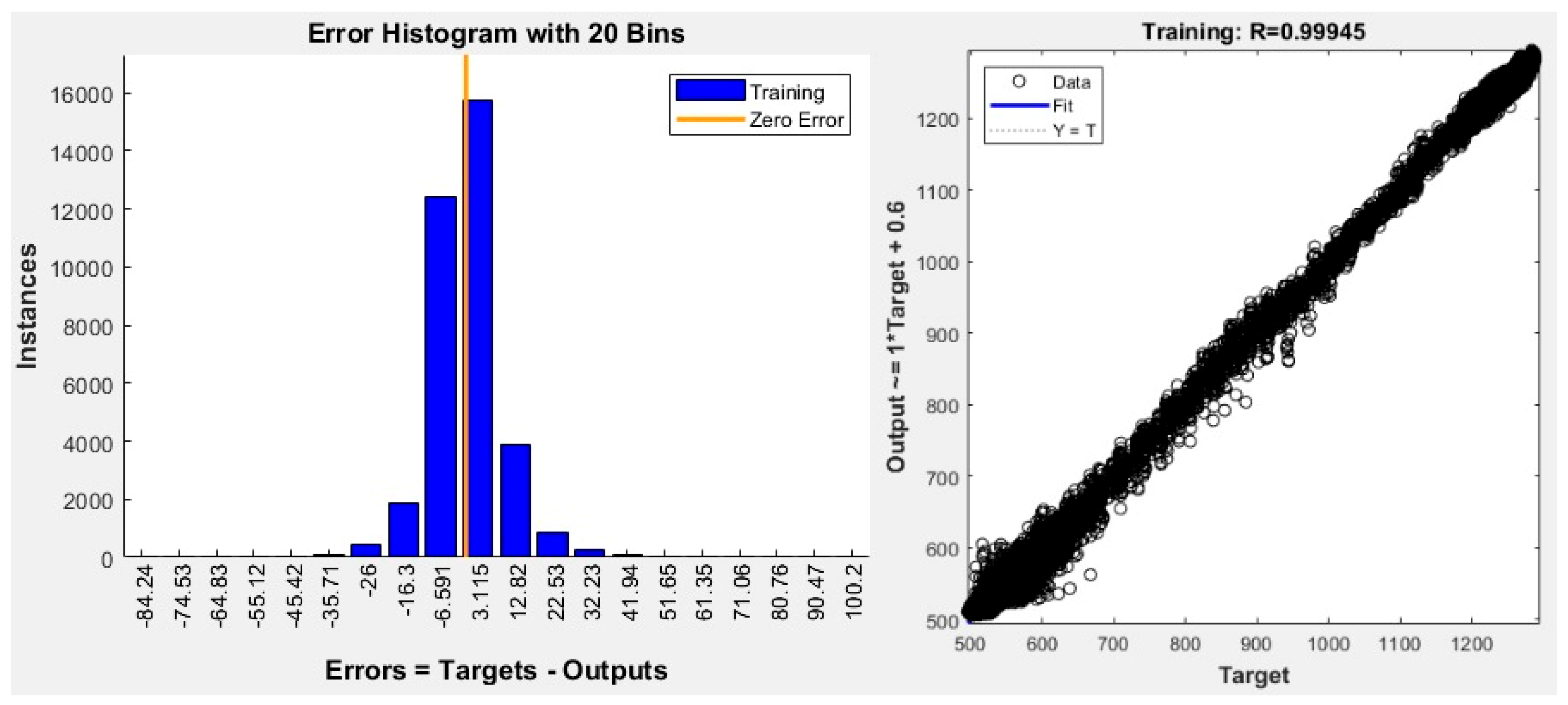
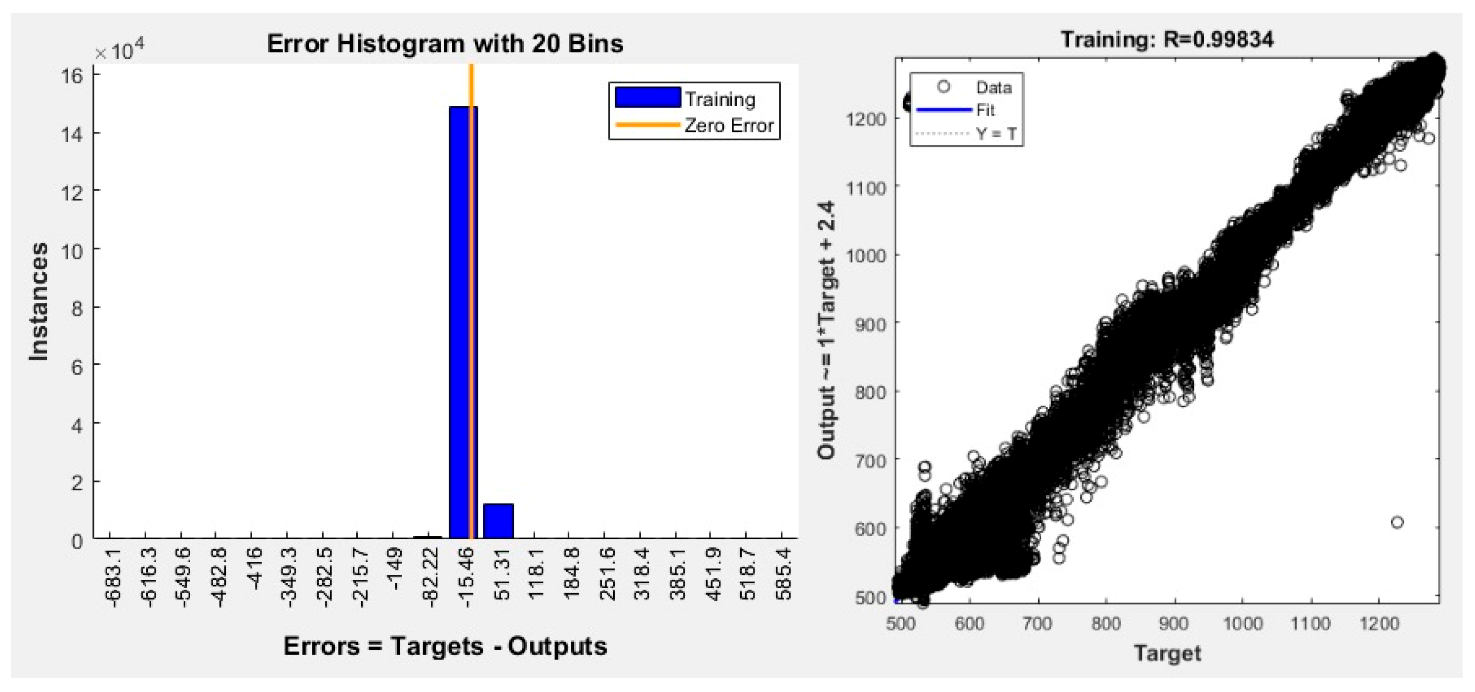
As shown in Figure 10, the training is successful, with good correlation between the inputs and the outputs after 1000 epochs. Validation also shows a good fit, with MSE = 100.26 K2, MRE = 1.03%, and MAE = 6.69 K, for an overall value range of 500–1300 K. Given this range, the results demonstrate a clear correlation between the selected dataset and the residual temperature of the part. The histogram, in particular, shows very small deviations from the target values, with the overwhelming majority of outputs not drifting more than 10 K from the target.

4.2. Robustness to Geometry Changes

In this test, the model is trained with the four orthogonal orientations of the original benchmark part, while the validation is performed with the altered part. Table 2 reports the training results for varying epoch counts, with the best result at 5000 epochs (MSE = 300.47 K2, MRE = 1.27%, and MAE = 9.73 K), after which validation performance degrades, indicating overfitting. While performance drops relative to the baseline, this was expected due to the increased variance between the training data and the validation data, and it remains within an acceptable range.

4.3. Input Significance Verification

In the validation and performance plot shown in Figure 11, where the model is trained using only element height as input, large deviations appear, and performance quickly stabilizes at a very high error. This makes it clear that outliers to the trend of temperature increasing with layer height cannot be predicted without adding the geometrical data to the inputs.
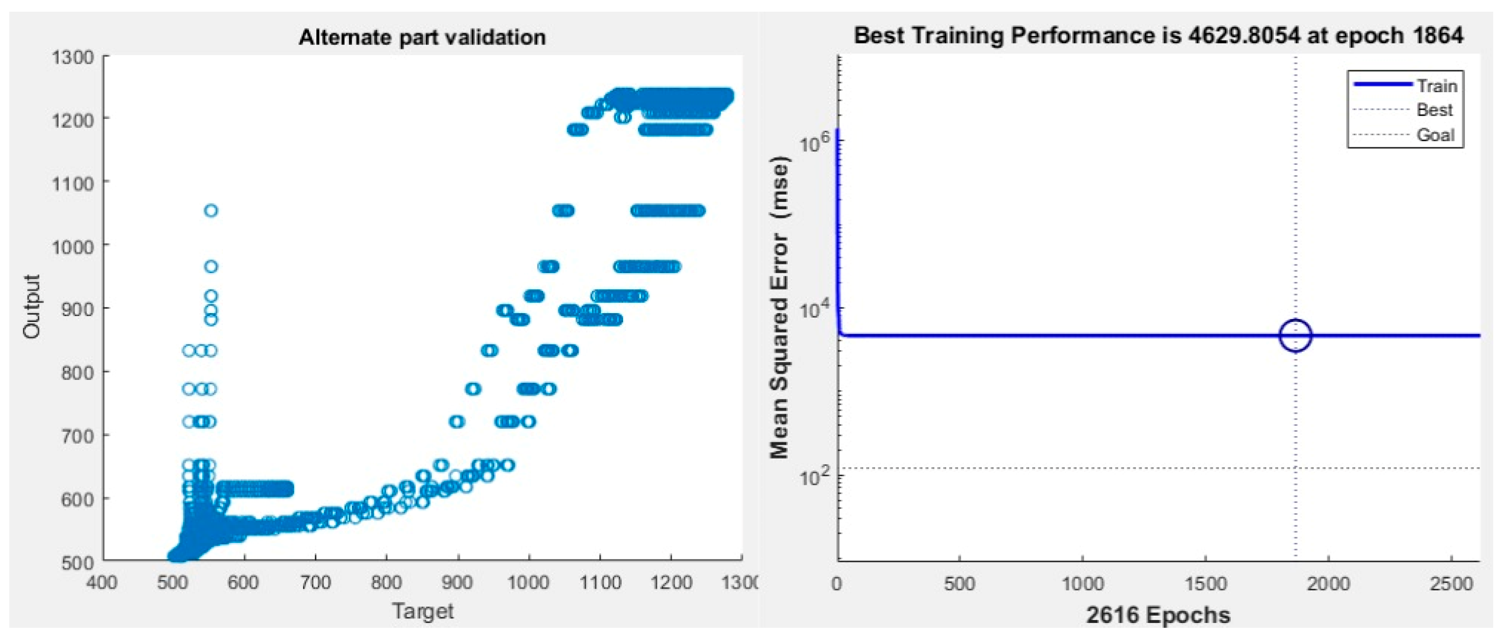
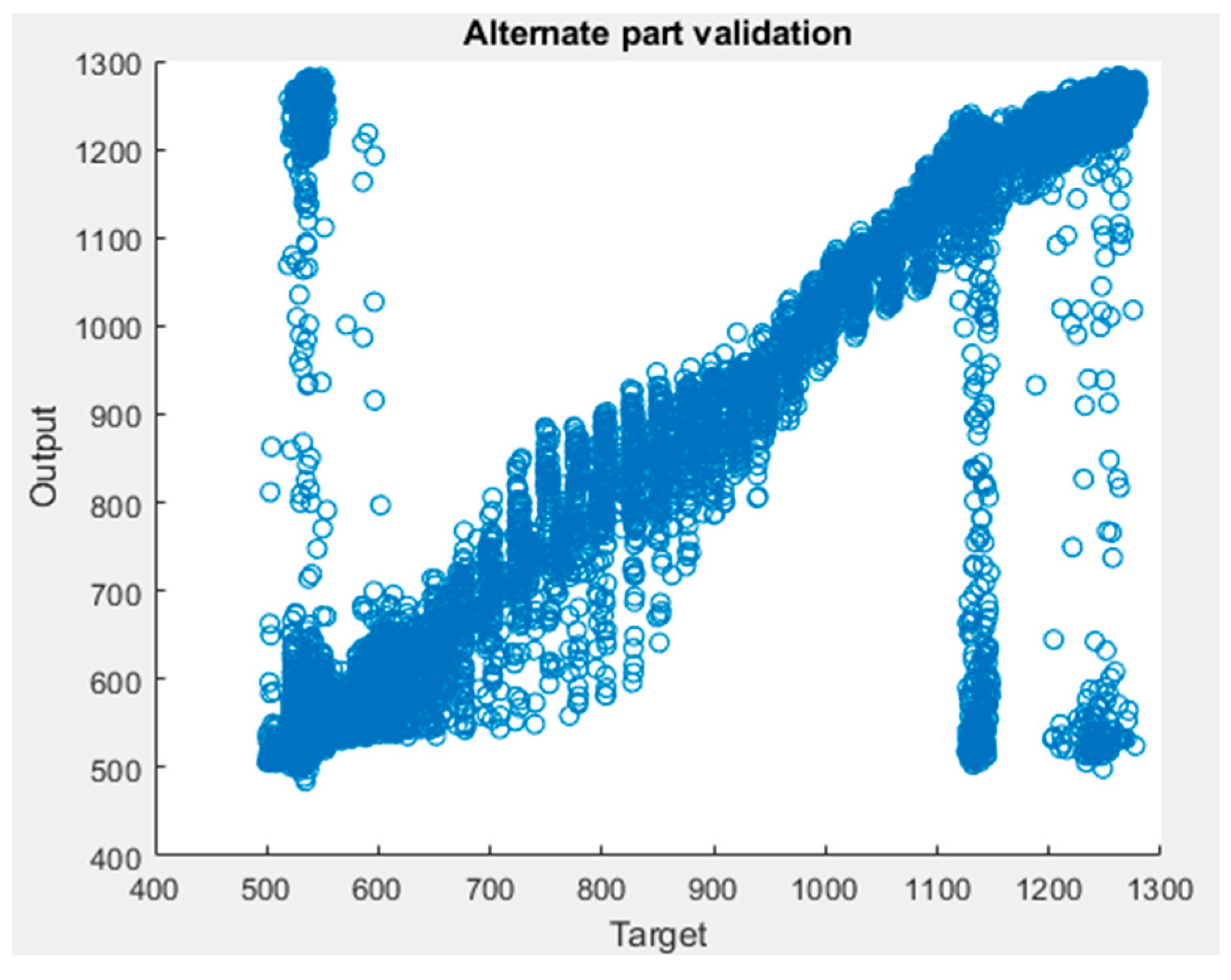
When omitting the height input instead (see the regression plot and error histogram in Figure 12), the network appears to have been successfully trained to an extent; however, the validation plot (see Figure 13) shows that the neural network is unable to properly correlate the geometrical data with the temperature values. A possible reason for the apparent accuracy in the middle temperature range is the fact that the benchmark part’s features differ sufficiently along the Y-axis that the neural network can (incorrectly) attribute the temperature difference solely to that factor, which is a false correlation.

4.4. Multi-Size Dataset Test

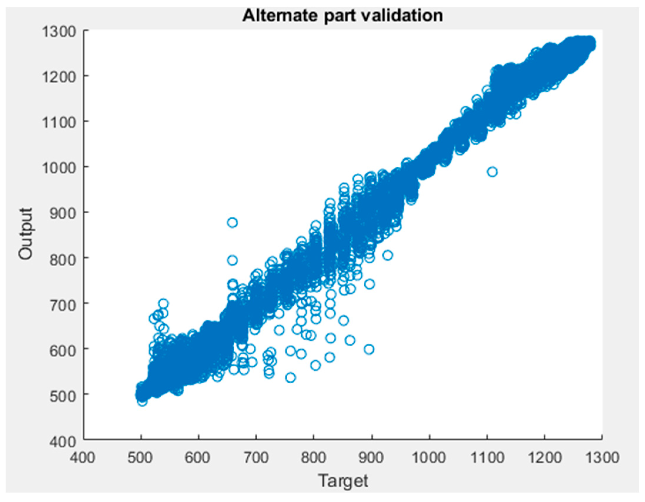
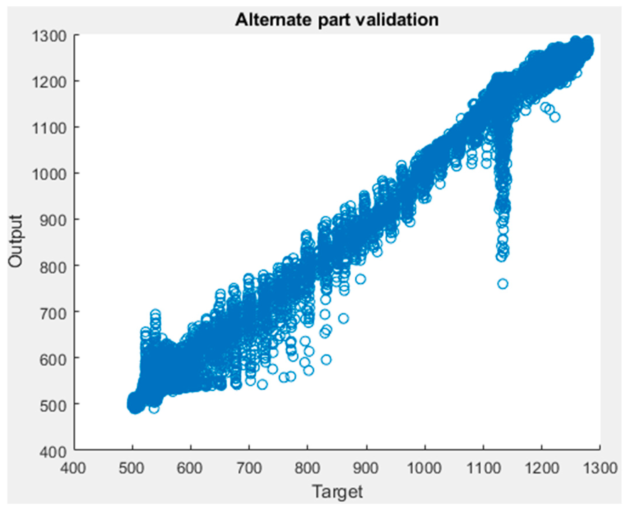
When training with the addition of smaller parts to the dataset, the training results are once again good, with the regression and validation plots shown in Figure 14. The resulting validation performance can be described by MSE = 47.07 K2, MRE = 0.74%, and MAE = 4.83 K. When tested using the alternative part, the DNN once again provides satisfactory—albeit worse than in previous testing—results: MSE = 326.84 K2, MRE = 1.33%, and MAE = 10.16 K, with the validation plot shown in Figure 15. This demonstrates the ability of the DNN to be trained for multiple-sized parts with different post-printing temperature ranges simultaneously while retaining sufficient accuracy. It is evident, however, that introducing more part sizes weakens the accuracy of the model, highlighting a limitation in scalability and generalization for even larger parts. Furthermore, Figure 16 shows validation results from training with the same parameters but without additional size input. An obvious mismatch between target and output values is observed, confirming the need for the additional size input when simultaneously training for differently sized parts, as expected.

5. Discussion

The geometry transform method proved effective in describing part geometry for use in neural network-based temperature prediction. Notably, the time required for the geometry transform and for inference is an order of magnitude less than executing a finite element simulation—requiring seconds rather than minutes or hours.
This method could be used to adjust print parameters or part design based on the predicted temperature, which is closely tied to part geometry as well as laser power and speed, these parameters having the most significant effect on the final mechanical properties of a printed part [24]. For instance, such hotspots could be mitigated by implementing a variable-power laser which reduces power when scanning potential hotspot regions to avoid the aforementioned effect. Furthermore, part orientation, part arrangement on the build plate (in case of multiple parts), scanning strategies, or support placement might need to be experimented with to achieve a more homogenous residual temperature field. Additional parameters that could be adjusted, in cases of excessive spatial gradients in the residual temperature field, may include chamber temperature, plate heating, and recoating cycle time.
In terms of quality assurance, the temperature field at the end of a build can signal necessity for targeted inspection actions, e.g., X-ray tomography, ultrasound, surface scanning, or post-print stress-relief treatment. Moreover, when implementing digital product passports, a predicted residual temperature field can serve as one of the pertinent fields indicating process consistency.
On a complementary line, determining the residual temperature gradients of a printed part during the design process can also help identify areas where heat has the biggest difficulty dissipating. Thus, in a ‘Design for Additive Manufacturing’ approach, geometrical adjustments can be made to the part to eliminate such areas and thus avoid the formation of temperature hotspots during printing, which are known to cause layer drift and defects [25].
Assuming a strong correlation between part geometry and the examined part quality properties, this method can also be a viable means of neural network training for processes other than SLM. In most manufacturing processes of a thermal nature, such as casting and welding, part geometry significantly influences the final part’s properties. Following this logic, after adapting the method to each process and incorporating complementary, process-specific inputs, the method could also be used in conjunction with existing process parameter-based neural networks to improve quality (including dimensional accuracy) of parts with varying geometrical characteristics. To the authors’ knowledge, current research does not yet offer any methods similar to the one developed in this study, making it a notable advancement in the field.

6. Conclusions

In the proposed method, geometry is encoded using a cluster of CVs around a point of interest, whose spatial intersections with the part are quantified and used as descriptor values. This data is then used to train a DNN along with simulated residual temperature data, serving as a surrogate for finite element simulations in this role. Using this method, residual temperature prediction accuracies of around 1% MRE and 10 K MAE are achieved over a temperature range of 500–1300 K, on unseen but similar parts, even when different-sized parts are included in the dataset. This enables potential use of the method in industry to rapidly identify potential hotspots in SLM as early as the design stage, and more generally for other processes where part geometry plays a crucial role.
While the DNN is trained on FE simulation results—and will therefore reflect any errors or biases in those data—this work’s contribution is a general methodology that can be trained on ground-truth from either simulations or experiments. We demonstrate the approach with the data currently available. The model’s high performance relative to these data—however accurate they are—shows the utility of the method
While the results of this study are promising, the method is still unsuitable for a wide variety of part sizes and is hindered by the coarse mesh of the original FE simulations and by descriptors tailored to the corresponding large element size. Future work should improve the accuracy and scalability of the method and add more functionality, such as variable CV sizing to better accommodate features spanning different scales. Building on the current concept, including training data with in situ, mid-print temperatures could provide more informative outputs and deeper insight into thermal phenomena during printing.
Another direction for expansion entails explainability, e.g., exploring whether certain control volumes in specific spatial positions (e.g., directly below or above the point of interest) consistently influence the prediction.
Spatial differences in residual temperatures imply differences in cooling paths, which could be correlated, e.g., via machine learning, to residual stresses, deformation, and even microstructure, and hence to hardness/strength, etc., avoiding their computationally heavy numerical calculation. This is an ambitious future extension of this work whose feasibility needs close examination.

Author Contributions

Conceptualization, N.P. and E.S.; methodology, N.P.; software, N.P.; validation, N.P., E.S. and G.-C.V.; writing—original draft preparation, N.P.; writing—review and editing, N.P., E.S. and G.-C.V.; visualization, N.P.; supervision, E.S. and G.-C.V.; funding acquisition, G.-C.V. All authors have read and agreed to the published version of the manuscript.

Funding

This research was partly funded by the European Union under Grant Agreement No. 101091783, project ‘MARS: Manufacturing Architecture for Resilience & Sustainability’, HORIZON-CL4-2022-TWIN-TRANSITION-01-03.

Data Availability Statement

The raw data supporting the conclusions of this article will be made available by the authors on request.

Conflicts of Interest

The authors declare no conflicts of interest.

Abbreviations

The following abbreviations are used in this manuscript:
SLMSelective Laser Melting
FEFinite-Element
NNNeural Network
GD&TGeometric Dimensioning and Tolerancing
DNNDeep Neural Network
MSEMean Squared Error
MREMean Relative Error
MAEMean Absolute Error
CSVComma-Separated Values

References

  1. Kurzynowski, T.; Pawlak, A.; Smolina, I. The Potential of SLM Technology for Processing Magnesium Alloys in Aerospace Industry. Arch. Civ. Mech. Eng. 2020, 20, 23. [Google Scholar] [CrossRef]
  2. Buchbinder, D.; Schleifenbaum, H.; Heidrich, S.; Meiners, W.; Bültmann, J. High Power Selective Laser Melting (HP SLM) of Aluminum Parts. Phys. Procedia 2011, 12, 271–278. [Google Scholar] [CrossRef]
  3. Loh, L.-E.; Chua, C.-K.; Yeong, W.-Y.; Song, J.; Mapar, M.; Sing, S.-L.; Liu, Z.-H.; Zhang, D.-Q. Numerical Investigation and an Effective Modelling on the Selective Laser Melting (SLM) Process with Aluminium Alloy 6061. Int. J. Heat Mass Transf. 2015, 80, 288–300. [Google Scholar] [CrossRef]
  4. King, W.; Anderson, A.T.; Ferencz, R.M.; Hodge, N.E.; Kamath, C.; Khairallah, S.A. Overview of Modelling and Simulation of Metal Powder Bed Fusion Process at Lawrence Livermore National Laboratory. Mater. Sci. Technol. 2015, 31, 957–968. [Google Scholar] [CrossRef]
  5. Ganeriwala, R.K.; Hodge, N.E.; Solberg, J.M. Towards Improved Speed and Accuracy of Laser Powder Bed Fusion Simulations via Multiscale Spatial Representations. Comput. Mater. Sci. 2021, 187, 110112. [Google Scholar] [CrossRef]
  6. Jimenez Abarca, M.; Darabi, R.; de Sa, J.C.; Parente, M.; Reis, A. Multi-Scale Modeling for Prediction of Residual Stress and Distortion in Ti–6Al–4V Semi-Circular Thin-Walled Parts Additively Manufactured by Laser Powder Bed Fusion (LPBF). Thin-Walled Struct. 2023, 182, 110151. [Google Scholar] [CrossRef]
  7. Nagesha, B.K.; Anand Kumar, S.; Vinodh, K.; Pathania, A.; Barad, S. A Thermo-Mechanical Modelling Approach on the Residual Stress Prediction of SLM Processed HPNGV Aeroengine Part. Mater. Today Proc. 2021, 44, 4990–4996. [Google Scholar] [CrossRef]
  8. Qi, X.; Chen, G.; Li, Y.; Cheng, X.; Li, C. Applying Neural-Network-Based Machine Learning to Additive Manufacturing: Current Applications, Challenges, and Future Perspectives. Engineering 2019, 5, 721–729. [Google Scholar] [CrossRef]
  9. Feng, F.; Zhu, T.; Yang, B.; Zhou, S.; Xiao, S. A Physics-Informed Neural Network Approach for Predicting Fatigue Life of SLM 316L Stainless Steel Based on Defect Features. Int. J. Fatigue 2024, 188, 108486. [Google Scholar] [CrossRef]
  10. Demir, K.; Zhang, Z.; Ben-Artzy, A.; Hosemann, P.; Gu, G.X. Laser Scan Strategy Descriptor for Defect Prognosis in Metal Additive Manufacturing Using Neural Networks. J. Manuf. Process 2021, 67, 628–634. [Google Scholar] [CrossRef]
  11. Xing, W.; Lyu, T.; Chu, X.; Rong, Y.; Lee, C.-G.; Sun, Q.; Zou, Y. Recognition and Classification of Single Melt Tracks Using Deep Neural Network: A Fast and Effective Method to Determine Process Windows in Selective Laser Melting. J. Manuf. Process 2021, 68, 1746–1757. [Google Scholar] [CrossRef]
  12. Gao, J.; Wang, C.; Hao, Y.; Wang, X.; Zhao, K.; Ding, X. Prediction of Molten Pool Temperature and Processing Quality in Laser Metal Deposition Based on Back Propagation Neural Network Algorithm. Opt. Laser Technol. 2022, 155, 108363. [Google Scholar] [CrossRef]
  13. Wang, C.; Tan, X.P.; Tor, S.B.; Lim, C.S. Machine Learning in Additive Manufacturing: State-of-the-Art and Perspectives. Addit. Manuf. 2020, 36, 101538. [Google Scholar] [CrossRef]
  14. Wang, Z.; Yang, W.; Liu, Q.; Zhao, Y.; Liu, P.; Wu, D.; Banu, M.; Chen, L. Data-Driven Modeling of Process, Structure and Property in Additive Manufacturing: A Review and Future Directions. J. Manuf. Process 2022, 77, 13–31. [Google Scholar] [CrossRef]
  15. Wu, S.-H.; Tariq, U.; Joy, R.; Sparks, T.; Flood, A.; Liou, F. Experimental, Computational, and Machine Learning Methods for Prediction of Residual Stresses in Laser Additive Manufacturing: A Critical Review. Materials 2024, 17, 1498. [Google Scholar] [CrossRef] [PubMed]
  16. Belongie, M. Matching with Shape Contexts. In Proceedings of the IEEE 2000 Proceedings Workshop on Content-based Access of Image and Video Libraries, Washington, DC, USA, 16 June 2000; pp. 20–26. [Google Scholar]
  17. Angrish, A.; Bharadwaj, A.; Starly, B. MVCNN++: Computer-Aided Design Model Shape Classification and Retrieval Using Multi-View Convolutional Neural Networks. J. Comput. Inf. Sci. Eng. 2021, 21, 011001. [Google Scholar] [CrossRef]
  18. Bacciaglia, A.; Ceruti, A.; Liverani, A. A Systematic Review of Voxelization Method in Additive Manufacturing. Mech. Ind. 2019, 20, 630. [Google Scholar] [CrossRef]
  19. Wang, Z.; Lu, F. VoxSegNet: Volumetric CNNs for Semantic Part Segmentation of 3D Shapes. IEEE Trans. Vis. Comput. Graph. 2020, 26, 2919–2930. [Google Scholar] [CrossRef]
  20. Giganto, S.; Martínez-Pellitero, S.; Cuesta, E.; Zapico, P.; Barreiro, J. Proposal of Design Rules for Improving the Accuracy of Selective Laser Melting (SLM) Manufacturing Using Benchmarks Parts. Rapid Prototyp. J. 2022, 28, 1129–1143. [Google Scholar] [CrossRef]
  21. Taylor, H.C.; Garibay, E.A.; Wicker, R.B. Toward a Common Laser Powder Bed Fusion Qualification Test Artifact. Addit. Manuf. 2021, 39, 101803. [Google Scholar] [CrossRef]
  22. Subbaian Kaliamoorthy, P.; Subbiah, R.; Bensingh, J.; Kader, A.; Nayak, S. Benchmarking the Complex Geometric Profiles, Dimensional Accuracy and Surface Analysis of Printed Parts. Rapid Prototyp. J. 2019, 26, 319–329. [Google Scholar] [CrossRef]
  23. Chen, Y.; Zhou, L.; Tang, Y.; Singh, J.P.; Bouguila, N.; Wang, C.; Wang, H.; Du, J. Fast Neighbor Search by Using Revised K-d Tree. Inf. Sci. 2019, 472, 145–162. [Google Scholar] [CrossRef]
  24. Hanzl, P.; Zetek, M.; Bakša, T.; Kroupa, T. The Influence of Processing Parameters on the Mechanical Properties of SLM Parts. Procedia Eng. 2015, 100, 1405–1413. [Google Scholar] [CrossRef]
  25. Yadav, P.; Rigo, O.; Arvieu, C.; Le Guen, E.; Lacoste, E. Data Treatment of In Situ Monitoring Systems in Selective Laser Melting Machines. Adv. Eng. Mater. 2021, 23, 2001327. [Google Scholar] [CrossRef]
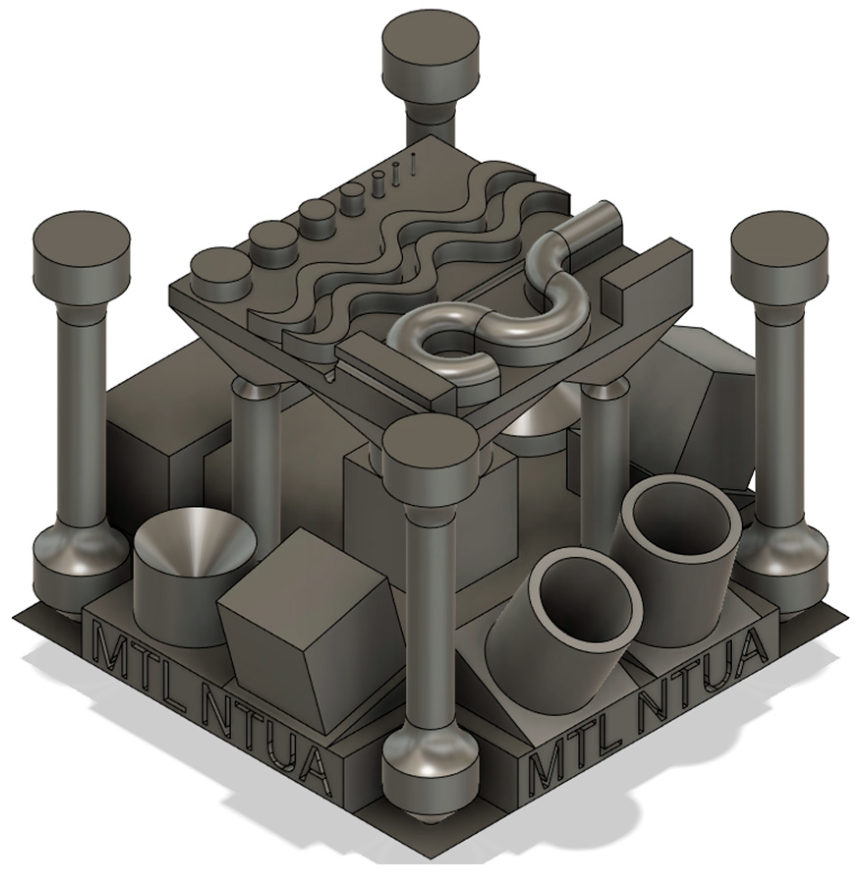
Figure 1. Full benchmark part. Bounding box dimensions: 55.5 × 54.1 × 41.6 mm.
Metals 15 01119 g001
Figure 2. Cubical CV intersection with benchmark part.
Metals 15 01119 g002
Figure 3. Possible placement of even number of CVs.
Metals 15 01119 g003
Figure 4. Possible placement of odd number of CVs.
Metals 15 01119 g004
Figure 5. Scatter plot of shape array compared to benchmark part.
Metals 15 01119 g005
Figure 6. Indicative simulation results of residual temperature field.
Metals 15 01119 g006
Figure 7. Part data extraction workflow.
Metals 15 01119 g007
Figure 8. Altered benchmark part compared to original.
Metals 15 01119 g008
Figure 9. Smaller sized parts used for simultaneous training.
Metals 15 01119 g009
Figure 10. Full benchmark part temperature training histogram and regression.
Metals 15 01119 g010
Figure 11. Training results for pure element height input.
Metals 15 01119 g011
Figure 12. Temperature training errors in histogram and regression plot with height input omission.
Metals 15 01119 g012
Figure 13. Altered benchmark part validation with height input omission during training.
Metals 15 01119 g013
Figure 14. Training regression and validation plots with multiple-sized parts.
Metals 15 01119 g014
Figure 15. Alternative part validation when training with multiple-sized parts.
Metals 15 01119 g015
Figure 16. Alternative part validation when training with multiple-sized parts without the size input.
Metals 15 01119 g016
Table 1. Altair print3D simulation parameters.
ParameterValue
Analysis typeThermo-mechanical
Velocity1.2 m/s
Laser power600 W
Powder layer thickness3 × 10−5 m
Powder absorption9%
Cooling time10 s
Base temperature298 K
Element size (length and height)0.001 m
Table 2. Altered benchmark part temperature prediction testing results.
EpochsMSE (K2)MREMAE (K)
1000398.261.58%11.87
2000354.761.39%10.67
3000355.901.36%10.39
4000339.801.31%10.15
5000300.471.27%9.73
6000356.581.34%10.35
Disclaimer/Publisher’s Note: The statements, opinions and data contained in all publications are solely those of the individual author(s) and contributor(s) and not of MDPI and/or the editor(s). MDPI and/or the editor(s) disclaim responsibility for any injury to people or property resulting from any ideas, methods, instructions or products referred to in the content.