Review

An Overview of Estimations for the High-Cycle Fatigue Strength of Conventionally Manufactured Steels Based on Other Mechanical Properties

by
Robin Motte
and
Wim De Waele
*
Soete Laboratory, Department of Electromechanical, Systems and Metal Engineering, Faculty of Engineering and Architecture, Ghent University, Technologiepark 46, BE-9052 Zwijnaarde, Belgium
*
Author to whom correspondence should be addressed.
Metals 2024, 14(1), 85; https://doi.org/10.3390/met14010085
Submission received: 23 October 2023 / Revised: 26 December 2023 / Accepted: 26 December 2023 / Published: 10 January 2024
(This article belongs to the Section Metal Failure Analysis)

Abstract

:
Due to the time-consuming and costly nature of high-cycle fatigue experiments, correlations between fatigue strength and mechanical properties obtained through more simple and fast experiments can be interesting from an economic perspective. This review article aims to provide an overview of such relations established in the open literature from the 1980s to 2023 for conventionally manufactured steel grades. The majority of these models relate fatigue strength at a given fatigue life (often termed “fatigue limit” or “endurance limit”) to ultimate tensile strength, yield strength (both static and cyclic), hardness, elongation, reduction in area, and Charpy impact energy. Relations taking flaws such as nonmetallic inclusions into account are also discussed. Additionally, models predicting S–N curves are provided. The various estimations are presented in tables, together with the materials and test conditions for which they were established.

1. Introduction

For many engineering structures, the fatigue resistance of a material is an important consideration during design. High-cycle fatigue of metal components refers to their sudden elastic fracture when subjected to alternating mechanical stress. The literature reports that 25% to 90% of mechanical failures are due to fatigue damage [1,2,3,4]. The elastic nature of this failure mechanism, i.e., without visual demonstration of component deformation, makes it difficult to detect. This poses significant potential risks to the users of such components. The importance of in-service fatigue failure of engineering structures is discussed in [5] based on several case studies.
It is without discussion primordial to analyse and accurately predict the fatigue performance of components during design. For instance, the German FKM guideline (Forschungskuratorium Maschinenbau) [6] is used in industry to assess the fatigue strength of machine components. The main tools of a fatigue design are the so-called S–N curve and a fatigue damage accumulation law. S–N curves (also called Wöhler curves) provide the number of load cycles to failure (N) as a function of applied stress level (S, denoted in this paper as σ F ) for a material or component. Basquin suggested a linear relationship between log σ F and log N such that σ F = C · N m [7]. S–N curves are typically determined by means of well-controlled laboratory experiments where test specimens are subjected to constant amplitude load cycles until failure. For example, ISO 1143:2021 describes the specimens and experimental procedure for rotating bending fatigue tests [8]. For a few metals, notably low- and medium-strength steels, the so-called fatigue limit has historically been an important consideration for fatigue design. At constant amplitude stress levels below the fatigue limit, these metals show infinite life. However, under in-service variable amplitude loading and/or environmental conditions such as corrosion, the fatigue limit is rare. While often used in the literature, the terms “fatigue limit” and “endurance limit” are not used in this paper, as there is ongoing debate about the existence of such phenomenon [9]. Moreover, fatigue failure has been observed beyond 10 6 and 10 7 cycles [9,10,11,12], where the fatigue limit is often defined. Therefore, the more general term “fatigue strength” (at a given fatigue life) is used in this review.
High-cycle fatigue experiments to characterize S–N curves or the fatigue strength at a given fatigue life are by nature time-consuming and often require a significant number of specimens, and are thus costly. For instance, establishing an S–N curve for design or reliability purposes according to ISO 12107:2012 requires a minimum of 30 observations [13]. Staircase testing to establish the fatigue strength at a given fatigue life also requires at least 30 experiments for reliability following the same standard. From an economic perspective, it can therefore be interesting to obtain an estimation of the fatigue strength of a material based on mechanical properties that can be more rapidly determined.
To illustrate the interest from researchers in this subject matter, Figure 1 shows the number of research articles in which such estimation was determined per year. The figure is based on the references used to draw up the tables in this review paper. Figure 2 shows the geographic distribution of the organizations affiliated with the first author of these same research papers. From this figure, it is clear that the majority of these publications originated in Chinese and Japanese institutions.
Section 2 presents estimations of the fatigue strength ( σ F ) based on other mechanical properties, such as ultimate tensile strength ( σ U ), yield strength ( σ Y ), and hardness (according to different scales). Additionally, estimations taking the effect of imperfections, such as nonmetallic inclusions into account, are also provided.
Section 3 describes various estimations for the S–N curve. Here, the estimations are discussed in a more chronological order. While a classification based on the considered material properties as in Section 2 is also possible, this approach allows for showing the relations between different estimations more clearly, as some were derived from others by using additional correlations.
It can be noted that estimations of the fatigue strength at a given fatigue life (such as those presented in Section 2) could also be determined by evaluating an estimation of the S–N curve (such as those presented in Section 3) at the desired fatigue life. However, Li et al. [14] recommended using a direct estimation of the fatigue strength rather than the indirect method of evaluating the S–N curve, based on an analysis of the fatigue strength at 10 6 cycles of 117 different steel alloys.
To distinguish between references, estimations for σ F and other equations, the following convention will be used:
  • “[X]” when referring to a source included in the list of references;
  • “Estimation X” when referring to a proposed estimation of σ F included in one of the tables;
  • “Equation (X)” when referring to an equation in the main body of the text.
Although it cannot be guaranteed that this paper contains a complete overview of all established estimations, it does provide estimations determined for various types of steels and different loading conditions from the 1980s until 2023. Furthermore, although estimations for low-cycle fatigue strength have been determined (for example, [15,16,17] list various estimations for different metals), the focus of this review is on correlations developed specifically for high-cycle fatigue properties of steel alloys.
It should be mentioned that the estimations presented in this paper are typically best-fit curves for a certain dataset and therefore not directly suited for design purposes, since conservatism was not considered during their derivation. Additionally, it is worth noting that models for the fatigue strength in the very high cycle regime were reviewed in [18], including probabilistic models for the S–N curve. Although several models will be discussed here as well, the focus of this review is on providing concrete predictions for the fatigue strength based on other mechanical properties.
While other papers (e.g., [19,20]) list multiple estimations for the high-cycle fatigue strength of steels (and other metals in [19]), this review paper aims to provide a more comprehensive overview. To improve the clarity and usability of this overview, the estimations are summarised in tables with particular attention to the materials and test conditions for which they were established (namely, stress ratio R, type of loading, and number of cycles at which the fatigue strength was determined), although it should be noted that full experimental details were not always provided. As material names were stated according to various national naming conventions, equivalent names according to the German naming convention and material numbers were obtained through the “Stahlschlüssel” [21] (when equivalent materials were available). To the authors’ knowledge, no overview with attention to these particular details has yet been published in open literature.

2. Estimations of the Fatigue Strength

2.1. Estimations Based on Ultimate Tensile Strength

Table 1 provides an overview of estimations of the high-cycle fatigue strength σ F based on ultimate tensile strength σ U . A common estimation of σ F at 10 6 cycles is 50 % of σ U [15], which was reportedly observed by Wöhler [22]. In [23], this estimation was considered suitable for ferrous metals with H B < 500 kgf / mm 2 loaded in bending. Analysis of data for 654 different steel alloys with σ U 1400 MPa by Meggiolaro and Castro [15] confirmed this proportionality. In addition to performing fatigue and tensile test experiments, the authors analysed material data from the ViDa software database. For steels with σ U 1400 MPa , a constant value of σ F = 700 MPa is commonly used as an upper limit for the linear relation [24]. However, when expanding their analysis to include higher-strength steels for a total of 724 steel alloys, Meggiolaro and Castro [15] found this to be an overly conservative estimation and determined that σ F = 0.49 · σ U better described the entire dataset. In [23], 1 / 3 · σ U was proposed to estimate σ F at 10 8 cycles for high-strength steels (and nonferrous metals) subjected to a bending load.
Roessle and Fatemi [24] performed uniaxial fatigue experiments and used data from ASM (American Society for Metals) to determine and evaluate the Coffin–Manson equation at 10 6 cycles, resulting in the estimation σ F = 0.38 · σ U . They noted that most high-cycle fatigue data are obtained through rotating bending tests, while their correlation is based on uniaxial tests, which result in a lower fatigue strength. While a bending load results in a stress gradient from the specimen’s centre to its surface, a uniaxial load causes a uniform stress distribution. Andersson [25] remarked that, as a rule of thumb, the fatigue strength for an axial load is 80% of that for a bending load. It should be noted that the approximation σ F = 0.49 · σ U resulting from Meggiolaro and Castro’s analysis was also based on uniaxial data, albeit for a larger variety of steels [15].
Electromagnetic resonance experiments on 42CrMo4 steel in [26] also led to the estimation σ F = 0.49 · σ U . However, the authors determined σ F for a fatigue life of around 10 7 cycles, with failures occurring between 10 6 and 10 7 cycles. Estimations 5, 6, and 7 were reported by the same authors for the same material subjected to different heat treatments (“AF” denoting “ausformed and tempered” and “QT” denoting “quenched and tempered”) and various loading conditions.
Analysis of NIMS (National Institute for Materials Science, Japan) data sheets for normalised carbon steels (with ferrite/pearlite microstructures) in [27] also resulted in estimation 5. Data for quenched and tempered steels (with tempered martensitic structure) from the same source led to estimation 8 [27]. In [28], estimations 10 to 13 were derived based on previous versions of the same data sheets from NRIM (National Research Institute for Metals, Japan). Yamaguchi et al. [29] also analysed the NRIM data and derived estimation 14, which differs from estimation 13 by 0.18%.
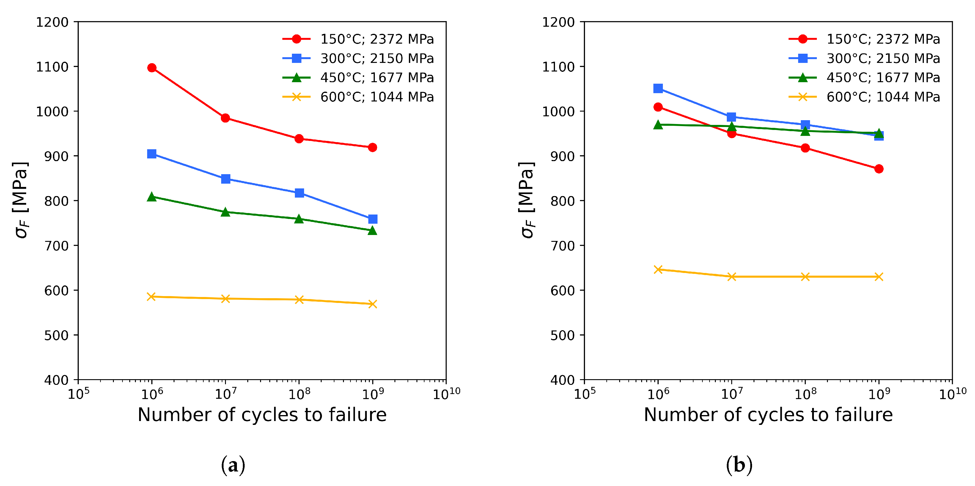
Zhao et al. [30] performed rotating bending and ultrasonic experiments on 100Cr6 steel at different tempering temperatures and collected data for low-alloy steels from the literature to establish estimations 15 and 16. While they defined “fatigue limit” as the fatigue strength at 10 7 cycles, they also noted a decrease in fatigue strength from 10 6 to 10 9 cycles (see Figure 3), thereby illustrating the importance of reporting the number of cycles where the fatigue strength was determined, rather than using only the term “fatigue limit”.
In [31], σ F was approximated based on Vickers hardness ( H V ):
σ F = 0.693 · H V + 85.05
Additionally, σ U and H V were correlated as
σ U = 2.82 · H V + 100
Combining these equations resulted in estimation 17. It should be noted that σ F was originally determined as the maximum stress during a fatigue cycle, but is presented here as a stress amplitude in order to be consistent with the other estimations in this review.
In his investigation of the high-cycle fatigue strength of a high-strength dual-phase steel sheet, Sperle [32] mentioned that the fatigue strength range at 10 6 cycles can be predicted as 80 % of σ U for untreated (meaning no prestraining or bake hardening) steels with σ U 500 MPa . While the original expression was derived for a stress range, it is given here as stress amplitude.
Table 1. Estimations for fatigue strength σ F based on ultimate tensile strength σ U .
No.EstimationMaterial aGerman Equivalent (Material Number) b [21]RcTest Type c,dNumber of Cycles cNotesRef.
1 σ F = 0.5 · σ U / −1RB, UA 10 6 [15,23]
2 σ F = 0.5 · σ U for σ U 1400 MPa
σ F = 700 MPa for σ U 1400 MPa
/ /// [24]
3 σ F = 1 3 · σ U / −1RB 10 8 [23]
4 σ F = 0.49 · σ U / −1UA 10 6 [15]
SCM440 (AF2000)42CrMo4 (1.7225)−1EMR 10 7 [26]
5 σ F = 0.43 · σ U Carbon steels normalised (ferrite/pearlite) /// [27]
SCM440 (QT2000)42CrMo4 (1.7225)−1US 10 8 [26]
6 σ F = 0.58 · σ U SCM440 (AF1600)42CrMo4 (1.7225)−1EMR 10 6 [26]
7 σ F = 0.55 · σ U SCM440 (QT1600)42CrMo4 (1.7225)−1US 10 7 [26]
8 σ F = 0.53 · σ U Carbon and low-alloy steels quenched and tempered (tempered martensite) /// [27]
9 σ F = 0.38 · σ U SAE 1141/−1UA 10 6 [24]
SAE 1038C35E (1.1181)
SAE 154136Mn6 (1.1127)
SAE 1050C50 (1.0540)
SAE 1090 C92D (1.0618)
10 σ F = 0.496 · σ U S25C (ferrite/pearlite structure)C25 (1.0406)−1RB/ [28]
11 σ F = 0.492 · σ U SUS304 (austenitic structure)X5CrNi18-10 (1.4301)−1RB/ [28]
12 σ F = 0.611 · σ U SUS430 (ferritic structure)X6Cr17 (1.4016)−1RB/ [28]
13 σ F = 0.542 · σ U S35CC35 (1.0501)−1RB/ [28]
S45C C45 (1.0503)
S55C C55 (1.0535)
SMn43836Mn6 (1.1127)
SMn44342Mn6 (1.1055)
SCr440 41Cr4 (1.7035)
SCM435 34CrMo4 (1.7220)
SCM44042CrMo4 (1.7225)
SNC631 36NiCr10 (1.5736)
SNCM43940NiCrMo6 (1.6565)
SNCM44734CrNiMo6 (1.6582)
14 σ F = 0.541 · σ U See estimation 13 −1RB 10 7 [29]
15 σ F = 0.468 · σ U GCr15 bearing steel Low alloy steels100Cr6 (1.3505)−1RB, US 10 7 [30]
16 σ F = 0.432 · σ U + 58.4 GCr15 bearing steel
Low-alloy steels
100Cr6 (1.3505)−1RB, US 10 7 [30]
17 σ F = 0.2475 · σ U + 60.3 SCr430B/0.1UA 2 · 10 6 to 3 · 10 6 [31]
SAE 1055C55 (1.0535)
Fe-18Mn-0.57C TWIP/
18 σ F = 0.4 · σ U Untreated steel 0UA 10 6 For σ U 500  MPa[32]
19 σ F = 0.36 · σ U 700/49/−1RB 10 7 [33]
20 σ F = 0.33 · σ U 900A/49/−1RB 10 7 [33]
21 σ F = 0.35 · σ U 900B/UIC60/−1RB 10 7 [33]
22 σ F = ( 0.70 1.85 · 10 4 · σ U ) · σ U SAE 434036CrNiMo (1.6511)−1US 10 9 [34]
23 σ F = ( 0.76 1.78 · 10 4 · σ U ) · σ U SAE 434036CrNiMo (1.6511)−1RB/ [34]
24 σ F = ( 0.87 2.65 · 10 4 · σ U ) · σ U SAE 414042CrMo4 (1.7225)−1RB/ [34]
25 σ F = ( 0.74 1.89 · 10 4 · σ U ) · σ U SAE 2340/−1RB/ [34]
26 σ F = ( 0.92 2.37 · 10 4 · σ U ) · σ U SAE 4063/−1RB/ [34]
27 σ F = ( 0.59 9.24 · 10 5 · σ U ) · σ U Alloy steels // 10 7 to 10 8 [19]
28 σ F = ( 0.67 1.52 · 10 4 · σ U ) · σ U Alloying steels −1US 10 9 [19,34]
29 σ F = ( 0.61 1.24 · 10 4 · σ U ) · σ U Wrought steels /// [34]
30 σ F = ( 0.60 2.13 · 10 4 · σ U ) · σ U Ultrafine and coarse-grained low-carbon steels /// [34]
31 σ F = 53 + 0.44 · σ U 0.00017 · σ U 2 Ductile cast steels −1RB 10 7 For σ U < 1400  MPa[25]
32 σ F = m · σ U · ( 2 · 10 7 ) b Ferrous powder metal materials /UA 10 7 m , b : material and postprocess treatment dependent[35]
a /: no specific material was provided in the original source; b /: no equivalent material was found; c /: not provided in the original source; d EMR: electromagnetic resonance; RB: rotating bending; UA: uniaxial; US: ultrasonic.
In [33], the fatigue strengths of three different railway steels were investigated. Estimations 19 to 21 were derived after performing static tensile tests and rotating bending fatigue tests up to 10 7 cycles. Although other estimations for the fatigue strength were listed, they are not included here as the original sources could not be found.
Pang et al. [34] observed a linearly decreasing relation between the ratio σ F σ U and σ U in experimental results for 36CrNiMo steel, as shown in Figure 4. Similar relations were determined based on data from the literature for different materials [19,34]. Therefore, the authors proposed a general model:
σ F = ( C P · σ U ) · σ U
The results of their analysis are summarised in estimations 22 to 30. Estimation 31 represents an additional quadratic relation between σ F and σ U reported by Andersson [25] for ductile cast steels with σ U < 1400 MPa.
Although this review focuses on conventionally manufactured steel alloys, it is worth mentioning that fatigue strength estimations have also been developed for steels produced by advanced processes. For example, Savu and Mourelatos [35] investigated the relation between high-cycle fatigue strength and σ U for ferrous powder metals, resulting in estimation 32 with the general formulation of σ F = m · σ U · ( 2 · 10 7 ) b . In this equation, m and b are material- and post-process-treatment-dependent parameters. For iron–carbon alloys in an as-sintered condition, m = 2.61 and b = 0.122 , resulting in σ F = 0.34 · σ U .

2.2. Estimations Based on Yield Strength

Approximations of σ F based on the (monotonic) yield strength σ Y are presented in Table 2. Pang et al. [19] derived estimation 33; however, they noted that there is no general relation between σ F and σ Y .
In [36], experimental S–N curves were established for dual-phase steel DP600. Evaluation of these curves and data from the literature for TRIP (transformation-induced plasticity) bainitic steel, 5083 aluminium, 17-4 PH stainless steel, and magnesium alloys allowed the derivation of estimation 34 [37]. Estimation 35 was established for TMCP (thermomechanical controlled processing) steels [38]. The fatigue strength at 10 7 cycles was determined by uniaxial tests at stress ratio R = 0.1 , and the Goodman mean stress correction equation was used to convert the result to R = 1 .
Liu et al. [39] established a correlation between yield strength, ultimate tensile strength, and fatigue strength in their “Y–T–F model” (yield strength–tensile strength–fatigue strength), which is discussed below in Section 2.3. The relation σ U = σ 0 + a · σ Y was used to eliminate σ U from the Y–T–F model, resulting in the simplified “Y–F model”:
σ F = σ Y ω · C σ Y σ 0 + a · σ Y
Apart from the ω and C parameters from the Y–T–F model, material-dependent values for σ 0 and a are required. For SAE 1141 (using the experimental data from [24]), the parameters were determined as C = 1.96 , ω = 2.09 , a = 0.58 , and σ 0 = 449 MPa.
Sperle and Nilsson [40] performed uniaxial fatigue experiments on various HSLA (high-strength low-alloy) steels and collected data from the literature (including [32,41]) to derive estimation 37 for un-notched specimens with a ground surface finish. Correction factors to account for notches and surface roughness were also provided. Additionally, an increase of 25% in fatigue strength was observed for stress ratio R = 1 . From resonance tests on dual-phase steels, Sperle determined estimation 38 [32]. Originally, the fatigue strengths in both cases were given in terms of stress range but are presented here as stress amplitude.
Yang et al. [42] established S–N curves for 34CrMo4 steel in different quenched and tempered conditions. The S–N curves were represented by the Basquin equation:
σ a = σ f · ( 2 · N f ) b
In this equation, σ a is the stress amplitude, N f is the number of cycles to failure, σ f is the fatigue strength coefficient, and b is the fatigue strength exponent. Equation (5) can be written in logarithmic form as
log σ a = log σ f + b · log 2 · N f
By correlating σ f and b in Equation (6) with the yield strength and evaluating the S–N curve at the knee point (between 10 6 and 10 7 cycles), they derived estimation 39.
In their investigation of railway steels, Krumes et al. [33] determined estimations 40 to 42.
Table 2. Estimations for fatigue strength σ F based on yield strength σ Y .
No.EstimationMaterial aGerman Equivalent (Material Number) b [21]RcTest Type c,dNumber of Cycles cNotesRef.
33 σ F = 0.22 · σ Y + 335 AISI 434034CrNiMo6 (1.6511)/// [19]
34 σ F = 0.6 · σ Y DP600/−1UA 10 6 [36,37]
TRIP bainitic steel
Al 5083
17-4 PH stainless steelX5CrNiCuNb16-4 (1.4542)
Mg alloys
35 σ F = 0.48 · σ Y + 165.25 TMCP steels −1UA 10 7 Data for R = 0.1 converted to R = 1 by Goodman equation[38]
36 σ F = σ Y 2.09 · 1.96 σ Y 449 + 0.58 · σ Y SAE 1141/−1UA 10 6 [24,39]
37 σ F = 38.2635 + 0.52735 · σ Y + 1.75 · 10 4 · σ Y 2 HS 310
HS 350
HS 390
HS 450
EHS 490
EHS 590
EHS 640
EHS 690
EHD 750
HS 420
EHS 900
/
/
/
/
/
/
/
/
/
/
/
0UA 10 6 [40]
38 σ F = 43.1495 + 1.064 · σ Y 0.144 · 10 2 · σ Y 2 + 0.0705 · 10 5 · σ Y 3 Mild steel 0R 10 6 [32]
DOCOL 400 BH/
DOCOL 600 DL/
DOCOL 600 /
DOCOL 800/
39 log σ F = ( 2.193 · 10 4 · σ Y 0.382 ) · ( 1.987 · 10 5 · σ Y 2 + 5.422 · 10 2 · σ Y 30.029 ) + log 2.542 · σ Y + 5564.850 35CrMo34CrMo4 (1.7220)−1UA 10 6 to 10 7 [42]
40 σ F = 0.69 · σ Y 700/49/−1RB 10 7 [33]
41 σ F = 0.63 · σ Y 900A/49/−1RB 10 7 [33]
42 σ F = 0.61 · σ Y 900B/UCI60/−1RB 10 7 [33]
a /: no specific material was provided in the original source; b /: no equivalent material was found; c /: not provided in the original source; d R: resonance; RB: rotating bending; UA: uniaxial.

2.3. Estimations Based on Ultimate Tensile Strength and Yield Strength

Table 3 presents three methods to predict σ F based on σ U and σ Y , with estimations 43 to 52 incorporating the yield ratio σ Y σ U . Sperle and Trogen performed experiments on HSLA steels and collected data from the literature [41] to establish the following estimation for the fatigue strength of un-notched, ground material:
σ F = 4.752 + 0.5605 · σ U 0.2605 · 10 3 · σ U 2
However, the authors reported a wide scatter in the experimental data, which may have been related to factors such as microstructure, residual stresses, variations in surface quality, and yield ratio [41]. Therefore, estimation 43 was derived in order to account for σ Y in addition to σ U . The fatigue strength given here has again been converted to a stress amplitude.
After collecting data for various steel alloys from the literature, Liu et al. [39] observed that for low values of σ U , σ F increased linearly with σ U . However, the authors noted that this relation does not hold for high-strength steels, with σ F decreasing for steels with σ U > 1500 MPa . Note that a validity limit of σ U 1400 MPa was suggested for the linear relation σ F = 0.5 · σ U (see Section 2.1, estimation 2). The authors suggested that the observed trend was caused by a decreased capacity for plastic deformation. To describe the plastic deformation capacity, the following parameter was proposed:
σ U σ Y σ U
The authors attempted to describe the dataset by considering different combinations of the variables σ F , σ Y , and σ U σ Y σ U . They determined that the ratios σ F σ Y and σ Y σ U were suitable to establish a linear relation, as shown in Figure 5. This linear expression was then transformed to the Y–T–F model given by
σ F = σ Y ω · C σ Y σ U
The general approach is similar to that of Pang et al. [34] in the sense that a linear relation is established for a dimensionless form of σ F ( σ F σ Y here and σ F σ U in [34]), from which an expression for σ F itself is derived. The fitting parameters ω and C are dependent on both the material and the loading conditions. The results for steel alloys are summarised in estimations 44 to 52.
In their extensive research regarding correlations between σ F and other mechanical properties, Pang et al. [19] obtained estimation 53 from the literature. Compared with experimental data for 34CrNiMo6, the prediction resulted in an error within 5%. However, the conditions under which this relation is valid are uncertain, as the original sources for neither the estimation itself nor the experimental data were found.

2.4. Estimations Based on Cyclic Yield Strength

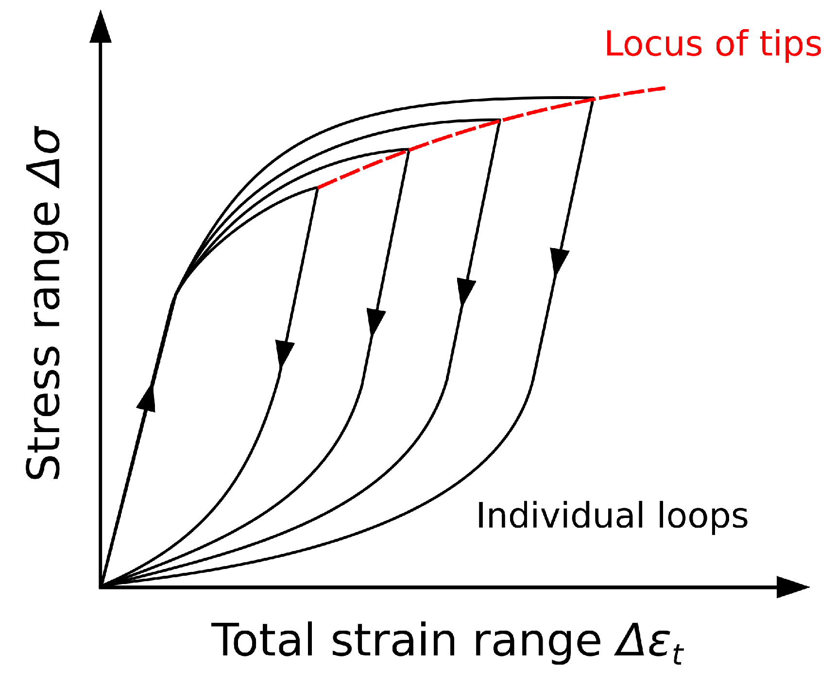
The previous sections described correlations between σ F and monotonic strength properties. However, a material may undergo cyclic hardening or softening during fatigue loading [28,37]. During strain-controlled testing, an increase in stress amplitude corresponds to cyclic hardening, while a decease in stress corresponds to cyclic softening [37]. Cyclic hardening occurs due to an increase in dislocation density, while cyclic softening occurs due to a decrease in dislocation density [28]. After a number of cycles, a stable stress–strain hysteresis loop is achieved, as shown in Figure 6 [28,37]. From these cyclic stress–strain data, a cyclic yield strength σ C Y can be defined. Table 4 lists several correlations between high-cycle fatigue strength and σ C Y .
It is important to note that different methods were used by different researchers to determine σ C Y . Paul [37] defined σ C Y as shown in Figure 6 by using a 0.01% offset in the loading branch of the hysteresis loop to determine 2 · σ C Y . However, Nishijima [28] and Li et al. [43] calculated σ C Y with a 0.2% offset in the cyclic stress–strain curve, while Socie et al. [23] mentioned a 0.1% offset. According to the guidance in [44], the cyclic stress–strain curve can be obtained as the locus of the tips of stable hysteresis loops at various strain ranges (after translation to a common origin point), as illustrated in Figure 7.
While estimations 54 (established by Paul [37] for a dual-phase steel) and 55 (proposed by Socie et al. [23] as an approximation for the fatigue strength of steel in bending) equate σ F and σ C Y , the three estimations derived by Nishijima [28] determine σ F as a smaller fraction of σ C Y . Apart from the investigated materials, the procedures to obtain σ C Y may also have contributed to these differences.
Li et al. [43] obtained σ C Y via the Ramberg–Osgood relation for cyclic stress–strain curves:
ϵ a = σ a E + σ a K 1 / n
As mentioned above, σ C Y was determined at a 0.2% plastic strain amplitude, resulting in
σ C Y = K · ( 0.002 ) n
The coefficients K and n were collected from the literature for several materials (including [24]). For their dataset, the relation between σ F and σ C Y was best described by the nonlinear equation given by estimation 59.
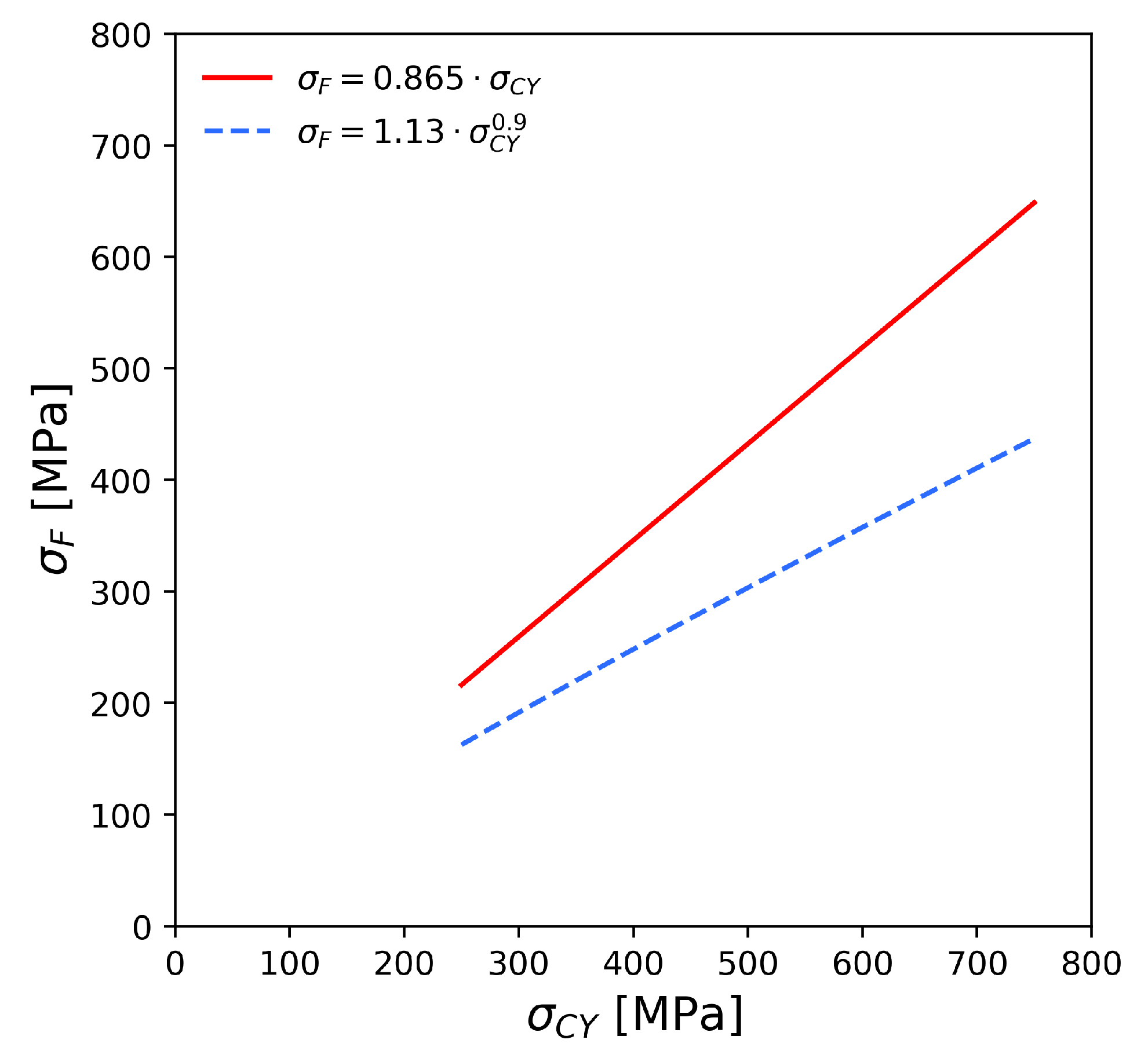
As estimations 58 and 59 were established for similar materials and for uniaxial tension–compression loading, a comparison is shown in Figure 8. Both estimations were evaluated for 250 MPa σ C Y 750 MPa as they were derived from data within a similar range. Within these bounds, σ F predicted by estimation 58 varies from 33% to 48% higher than σ F calculated from estimation 59.

2.5. Estimations Based on Vickers Hardness

Table 5 contains estimations of σ F based on Vickers hardness H V . A common rule of thumb for steels with H V < 400 kgf / mm 2 is to approximate σ F as 1.6 · H V [45,46,47]. This prediction is related to estimation 1, as Murakami and Endo [47] mentioned that σ F 0.5 · σ U 1.6 · H V . Considering this estimation suitable for the stress ratio R = 1 , Rigon and Meneghetti [46] derived the more general estimation 61 based on the Goodman mean stress correction equation.
Nishijima [28] determined proportionalities between σ F and H V under different load types, namely, reversed torsion (estimation 62), uniaxial loading (estimation 63), and rotating bending (estimation 64), based on data from the National Research Institute for Metals (NRIM). These estimations also indicate that reversed torsion is a more severe load type than uniaxial tension–compression or rotating bending, as a lower fatigue strength is obtained for the same value of H V . For rotating bending, additional data for stainless steels were considered to establish the linear relation between log ( σ F ) and log ( H V ) given by estimation 65. Analysis of data published by the Society of Materials Science, Japan (JSMS), in [48] resulted in estimations 66 to 68.
Mortezaei and Mashreghi [49] established S–N curves for different DIN steels, with plateaus around 10 6 to 10 7 cycles. The fracture surfaces of the failed specimens were investigated by scanning electron microscopy (SEM) in order to determine the dimensions of the inclusion where the fatigue crack initiated. Murakami’s estimation (described in Section 2.9) was used to calculate the stress intensity factor K I , m a x . The threshold stress intensity factor K I , t h was defined as the lowest value for K I , m a x calculated for each material. As it was assumed that no fatigue crack propagation occurs for stress intensity factors below this threshold value, it was used as a basis to estimate the “fatigue limit”. The following correlations were determined, from which estimation 69 was derived:
σ F = ( 158.46 · K I , t h ) + 125.51
K I , t h = ( 0.0046 · H V ) 0.010
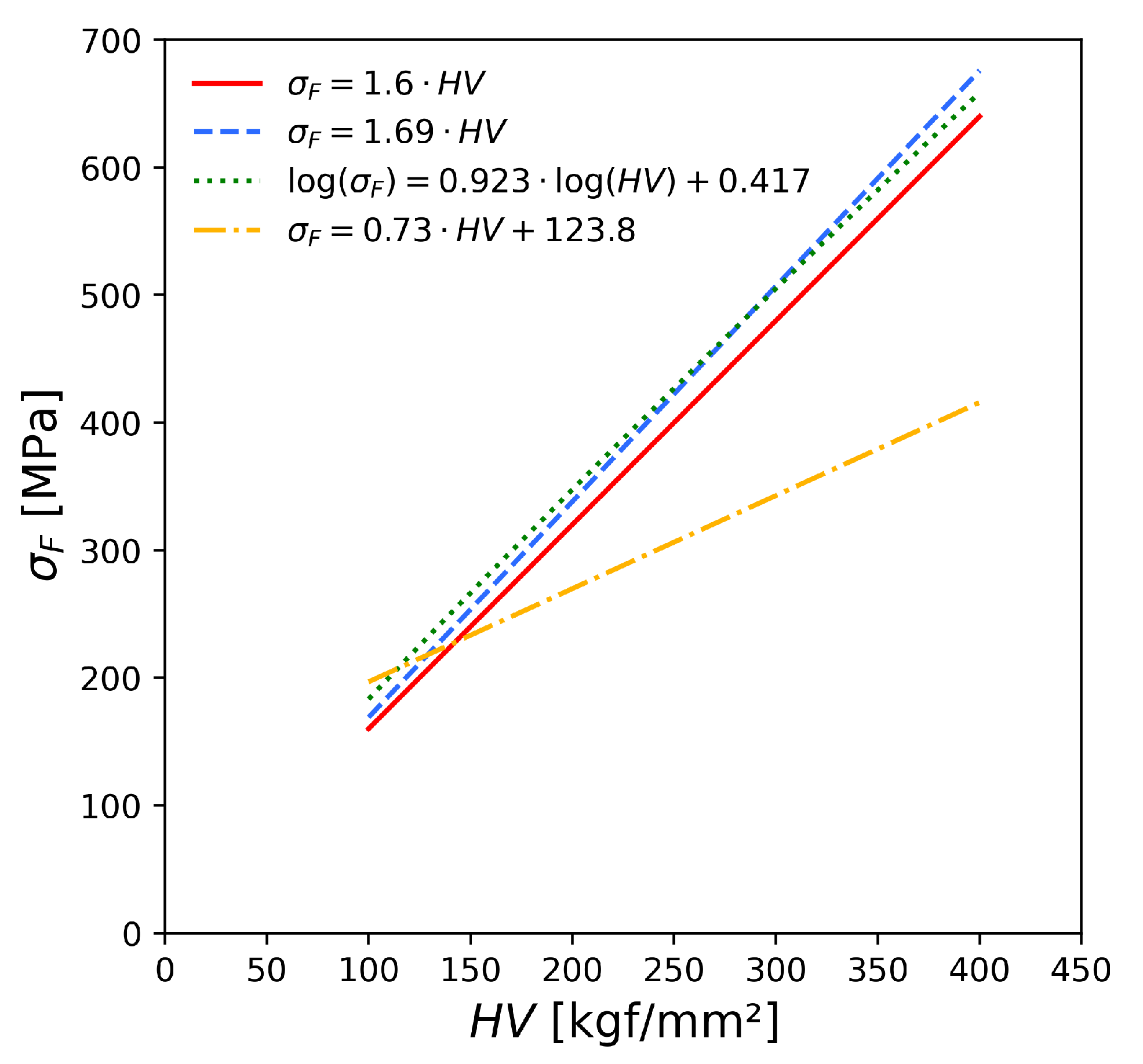
Figure 9 shows estimations 60, 64, 65, and 69 evaluated for 100 kgf / mm 2 H V 400 kgf / mm 2 . Estimation 64 results in a fatigue strength 6% higher than the common approximation of 1.6 · H V . The maximum difference of σ F obtained by estimation 65 and 1.6 · H V is 15% for the range of H V values considered in Figure 9. Compared with the other estimations shown, estimation 69 results in a considerably lower prediction for σ F , with a maximum difference of 35% within these bounds for H V .
In [50], Gao et al. investigated the fracture surfaces of an HSLA steel and determined that fatigue cracks initiated in the ferrite phase or at the boundary between ferrite and pearlite. The authors derived estimation 70 based on Murakami’s estimation (Section 2.9) by considering the average ferrite grain size as the a r e a parameter and the microhardness of pearlite.
Estimation 71 was originally established in [31] with σ F as the maximum stress, but is presented here as a stress amplitude. As this estimation was based on data for a fatigue load with a mean tensile stress ( R = 0.1 ), a lower σ F is predicted compared with the estimations established for R = 1 .
Similar to the quadratic relation between σ F and σ U (Equation (3)), Pang et al. [19] established estimations 72 (based on their experimental data in [34]) and 73 (based on data from the literature) as quadratic relations between σ F and H V .
Estimation 74 was developed for steels with various surface modifications in [51], and its applicability was verified in [52] for additional materials. Analysis of the failed specimens revealed that failure initiated in the substrate adjacent to the coating. During processes such as thermoreactive deposition and diffusion, chemical vapour deposition, and physical vapour deposition, tensile residual stresses arose in the substrate, with a detrimental effect on fatigue life. Additionally, carbide formation led to a decrease in hardness of the substrate due to carbon consumption [51].
Table 5. Estimations for fatigue strength σ F based on Vickers hardness H V .
No.EstimationMaterial aGerman Equivalent (Material Number) b [21]RcTest Type c,dNumber of Cycles cNotesRef.
60 σ F = 1.6 · H V ± 0.1 · H V Low- or medium-strength steels 1 RB or UA/For H V < 400 kgf / mm 2
Based on σ F = 0.5 · σ U
[45,46,47]
61 σ F = 3.2 · H V · 1 R 3 R / ///Based on σ F , R = 1 = 0.5 · σ U = 1.6 · H V and Goodman equation[46]
62 σ F = 1.13 · H V S35CC35 (1.0501)−1RT/ [28]
S45CC45 (1.0503)
S55CC55 (1.0535)
SMn43836Mn6 (1.1127)
SMn44342Mn6 (1.1055)
SCr44041Cr4 (1.7035)
SCM43534CrMo4 (1.7220)
SCM44042CrMo4 (1.7225)
SNC63136NiCr10 (1.5736)
SNCM43940NiCrMo6 (1.6565)
SNCM44734CrNiMo6 (1.6582)
63 σ F = 1.66 · H V See estimation 62 −1UA/ [28]
64 σ F = 1.69 · H V See estimation 62 −1RB/ [28]
65 log ( σ F ) = 0.923 · log ( H V ) + 0.417 ± 0.0197 S25CC25 (1.0406)−1RB/ [28]
S35CC35 (1.0501)
S45CC45 (1.0503)
S55CC55 (1.0535)
SMn43836Mn6 (1.1127)
SMn44342Mn6 (1.1055)
SCr44041Cr4 (1.7035)
SCM43534CrMo4 (1.7220)
SCM44042CrMo4 (1.7225)
SNC63136NiCr10 (1.5736)
SNCM43940NiCrMo6 (1.6565)
SNCM44734CrNiMo6 (1.6582)
SUS304X5CrNi18-10 (1.4301)
SUS430X6Cr17 (1.4016)
SUS403X6Cr13 (1.4000)
66 σ F = 1.7108 · H V S10C
S15C
S25C
C10E (1.1121)
C15E (1.1141)
C25 (1.0406)
−1RB 10 6 to 10 7 [48]
67 σ F = 1.4217 · H V S30C
S35C
S45C (EQT)
S50C (EQT)
C30 (1.0528)
C35 (1.0501)
C45 (1.0503)
C50 (1.0540)
−1RB 10 6 to 10 7 [48]
68 σ F = 1.6573 · H V S45C (Q&T)
S50C (Q&T)
C45 (1.0503)
C50 (1.0540)
−1RB 10 6 to 10 7 [48]
69 σ F = 0.73 · H V + 123.8 DIN 1.1186
DIN 1.1302
DIN 1.7218
DIN 1.7176
C40E
30MnVS6
25CrMo4
55Cr3
−1RB 10 6 to 10 7 For H V < 400 kgf / mm 2 [49]
70 σ F = 1.38 · H V P 35CrMo34CrMo4 (1.7220)−1EMR 10 7 H V P : microhardness of pearlite phase[50]
38MnVS /
71 σ F = 0.693 · H V + 85.05 SCr430B/0.1UA 2 · 10 6 to 3 · 10 6 [31]
SAE 1055C55 (1.0535)
Fe-18Mn-0.27C TWIP /
72 σ F = ( 2.42 2.21 · 10 3 · H V ) · H V AISI 434036CrNiMo4 (1.6511)−1US 10 9 [19,34]
73 σ F = ( 2.80 2.35 · 10 3 · H V ) · H V SUP760Si7 (1.5027)−1RB/ [19]
74 σ F = H V 10 + 20 · 9.8 1.04 · H V 1000 · σ r 414042CrMo4 (1.7225)−1PB, RB/Residual stress in substrate
Hardness at substrate’s surface
[51,52]
H13X40CrMoV5-1 (1.2344)
D2X153CrMoV12 (1.2379)
ASP30BSt 420 S (1.0428)
Surface modifications:
Hardening
VC coating
NbC coating
Cr-C coating
TiC coating
TiN coating
a /: no specific material was provided in the original source; b /: no equivalent material was found; c /: not provided in the original source; d EMR: electromagnetic resonance; PB: plane bending; RB: rotating bending; RT: reversed torsion; UA: uniaxial; US: ultrasonic.

2.6. Estimations Based on Brinell Hardness

Apart from H V , hardness on the Brinell scale ( H B ) has also been used as a basis for approximations of σ F as presented in Table 6. In [23], the common rule of thumb of σ F = 0.5 · σ U is estimated as 1.72 · H B for ferrous metals with H B < 500 kgf / mm 2 . Roessle and Fatemi [24] observed poor agreement of this estimation with their dataset and determined 1.43 · H B as an improved estimation. As mentioned in Section 2.1, the reduced fatigue strength may be the result of the different stress distribution in uniaxial tests as compared with rotating bending experiments. Pang et al. [19] mentioned that while estimation 77 is valid for H B < 400 kgf / mm 2 , it is not conservative for higher hardness.
The German FKM guideline approach to stress-based uniaxial fatigue analysis is described in detail in [53]. Only a general overview will be provided here. First, if no tensile test data for the material are available, the “mean σ U of a standard material test specimen” is estimated from H B as σ U = 3.45 · H B , after which a “reliability correction factor” C R and a “size correction factor” C D are applied. Without available experimental data, it is not possible to perform statistical analysis to quantify variability in the material’s strength, from which a conservative lower bound could be determined. Therefore, the correction factor C R is introduced, and its values are provided (based on the assumption of a normally distributed σ U ). For a survival rate of 97.5% (as recommended by the FKM guideline), C R = 0.843 . The aim of the factor C D is to account for the difference in dimensions between a test specimen and a real component. Its value is dependent on the material and dimensions of the component under consideration. Determining the fatigue strength at 10 6 cycles under reversed loading ( R = 1 ) requires two additional factors, namely, a “temperature correction factor” C E , T and an “endurance limit correction factor” C σ , E . Both factors are material dependent. Similar to C R , the values for C σ , E also account for 97.5% reliability. For example, C σ , E = 0.4 for forged steel. Assuming C D = C E , T = 1 , this results in σ F = 1.16 · H B . While this estimate appears lower than estimation 76 for identical load conditions, it should be noted that the FKM guideline approach is intended to be used for design purposes and therefore takes conservatism into account in the various correction factors (in particular, C R and C σ , E ).
Table 6. Estimations for fatigue strength σ F based on Brinell hardness H B .
No.EstimationMaterial aGerman Equivalent (Material Number) b [21]RcTest Type c,dNumber of Cycles cNotesRef.
75 σ F = 1.72 · H B / −1RB 10 6 For H B < 500 kgf / mm 2
Based on σ F = 0.5 · σ U
[23]
76 σ F = 1.43 · H B SAE 1141
/−1UA 10 6 [24]
SAE 1038C35E (1.1181)
SAE 154136Mn6 (1.1127)
SAE 1050C50 (1.0540)
SAE 1090C92D (1.0618)
77 σ F = 1.6 · H B / ///For H B < 400 kgf / mm 2 [19,54]
78 σ F = C σ , E · C E , T · C D · C R · 3.45 · H B / −1UA 10 6 C σ , E : endurance limit factor for normal stresses (material dependent)
C E , T : temperature correction for endurance limit (material dependent)
C D : size correction factor (material dependent)
C R : reliability correction factor
[53]
a /: no specific material was provided in the original source; b /: no equivalent material was found; c /: not provided in the original source; d RB: rotating bending; UA: uniaxial.

2.7. Estimations Based on Rockwell Hardness

Table 7 presents predictions of σ F based on hardness measurements on the Rockwell scales. In addition to the quadratic approximations based on σ U and H V described in Section 2.1 and Section 2.5, respectively, Pang et al. [19] also established relations based on H R C for different steel alloys, presented in estimations 79 to 83.
In their research regarding the fatigue strength of ferrous powder metals, Savu and Mourelatos [35] collected data from the literature for different materials. However, as hardness values were reported according to different scales (namely, H R B , H R C , and H R F ), they proposed the following pseudo- H R B scale:
H R B p = 0.004 · H R C 2 + 0.9 · H R C + 131.5 H R B 1.76 · H R F + 50.5
Analysis of the data suggested a good correlation between H R B p and σ U . As a relation between σ F and σ U was established (estimation 32), a similar equation was determined based on H R B p , resulting in estimation 84. H R B p is implemented in the form of a third-order polynomial with material-dependent coefficients. In case of iron–carbon alloys in an as-sintered condition, the coefficients are n a = 0.0023 , n b = 0.385 , and n c = 21.97 . As before, the exponent b = 0.122 .

2.8. Estimations Based on Multiple Properties

To capture the effect of multiple material characteristics on σ F , several researchers have developed estimations incorporating various properties, as shown in Table 8. Combinations of the following material properties were considered: σ U , σ Y , reduction in area ( ψ ), H B , Charpy impact energy ( C V N ), chemical composition ( C P ), and cyclic hardening exponent e I I .
Estimations 85 to 87 were established by Martinez et al. [55]. The original fatigue strengths were given in terms of stress ranges, but are presented here as amplitudes. These estimations are interesting as the Charpy impact energy ( C V N ) is implemented, thereby taking the material’s toughness into consideration. While all three estimations provide a good correlation with the dataset for which they were established, it is worth mentioning that a seemingly contradictory trend is present in estimation 85, as σ F increases with H B but decreases with σ U . However, Meggiolaro and Castro [15] reported that, based on an analysis of 1924 different steels, a strong correlation exists in the form of σ U = 3.4 · H B . Proportional relations between hardness and σ U were also at the basis of estimations 60, 61, and 75. In estimation 86, the variable C P represents the sum of the percentages of the alloying elements [55]:
C P = % ( C + M n + N i + C r + M o + V + T i + N b )
While the chemical composition of an alloy will certainly influence the mechanical performance, considering this numerical sum as a material property may be an oversimplification. In summary, while a good correlation may be obtained using these combinations of properties as variables in curve fits, the resulting equations do not always have a strong physical motivation.
In [56], data from [24,55] were used as a basis to establish the following relation:
σ F = 1.3 · H B + 0.02 · σ U
However, the validity of combining these datasets can be questioned as different stress ratios R were used in the original experiments (namely, R = 1 in [24] and R = 0 in [55]).
Estimations 88 to 90 relate σ F with a combination of σ U and the reduction in area ψ , thereby considering ductility in addition to static strength. Estimations 89 and 90 contain the product of σ U and ψ , which could be regarded as a metric for the toughness of the material, similar to the area below a stress–strain curve. In addition to their correlation between σ F and σ C Y (estimation 59), Li et al. [43] established the following relation between σ C Y , σ U , and ψ :
σ C Y = ( 1 + ψ ) · σ U · 0.002 ln ( 1 ψ ) 0.16
The substitution of this equation into estimation 59 resulted in estimation 90. As σ C Y was eliminated, the required material properties can be determined from static tensile tests.
In [25], an additional correlation was reported for the fatigue strength at 10 7 cycles of carbon and tempered steels with σ U < 1000 MPa subjected to rotating bending (estimation 91). It should be noted that ψ should be substituted here as a value in percent (e.g., 30%), while dimensionless numbers (e.g., 0.3) are required in estimations 88 to 90.
In addition to regular Vickers hardness tests, Görzen et al. [57] performed cyclic indentation tests while continuously monitoring the applied force F and indentation depth h. From the resulting Fh hysteresis loops, the plastic indentation depth amplitude h a , p was determined as the half width of the hysteresis loop at the mean load, as shown in Figure 10a. The definition of h a , p was made analogous to the definition of plastic strain amplitude in a stress–strain hysteresis curve (examples of which are shown in Figure 6 and Figure 7). To describe the material’s cyclic hardening behaviour, the evolution of h a , p versus the number of cycles N was considered. In the resulting h a , p N curve, the following power law was proposed to describe the second regime ( 5 N 10 , denoted by the subscript I I ):
h a , p I I = a I I · N e I I
The exponent e I I describes the slope of the second regime of the h a , p N curve and is considered a metric for the material’s cyclic hardening potential. Thus, it was termed the “cyclic hardening exponent”.
Figure 10. Definitions of (a) h a , p in the indentation force vs. indentation depth hysteresis loop and (b) h a , p I I based on the experimental plastic indentation depth amplitude as a function of the number of cycles [58]. Reproduced and adapted with permission from Schwich et al., Mater. Sci. Eng. A; published by Elsevier, 2020.
Metals 14 00085 g010
Table 8. Estimations for fatigue strength σ F based on multiple properties.
No.EstimationMaterial aGerman Equivalent (Material Number) b [21]RcTest Type c,dNumber of Cycles cNotesRef.
85 σ F = 0.085 · C V N + 1.295 · H B 0.205 · σ U AISI-SAE 4330M/0UA 5 · 10 6 [55]
AISI-SAE 4138M/
AISI-SAE 414042CrMo4 (1.7225)
86 σ F = 0.065 · C V N + 3.745 · C P 0.185 · σ U See estimation 85 0UA 5 · 10 6 C P = % ( C + M n + N i + C r + M o + V + T i + N b ) [55]
87 σ F = 0.675 · C V N 395.515 · σ Y σ U + 1.635 · H B See estimation 85 0UA 5 · 10 6 [55]
88 σ F = 0.39 · σ U + 100 · ψ / /// [43]
89 σ F = 0.25 · ( 1 + 1.35 · ψ ) · σ U High-strength steels /// [19]
90 σ F = 0.46 · ( 1 + ψ ) · σ U ln ( 1 ψ ) 0.16 0.9 SAE 1141/−1UA 10 6 [43]
SAE 1038C35E (1.1181)
SAE 154136Mn6 (1.1127)
SAE 1050C50 (1.0540)
SAE 1090C92D (1.0618)
08/
20/
30/
40/
40CrNiMo40NiCrMo6 (1.6565)
60Si2Mn60Si7 (1.5027)
91 σ F = 0.51 · σ U 1.67 · ( 64 ψ ) Carbon and tempered steels −1RB 10 7 For σ U < 1000 MPa
ψ as value in %
[25]
92 σ F = 4.82 · H V · | e I I | 7.18 100CrMnSi6-4
X0.5CuN2-2
X21CuNi2-2
C50E
42CrMo4
(1.3520)
/
/
(1.1206)
(1.7225)
1
1
1
/
1
UA
UA
UA
/
R
2 · 10 6
2 · 10 6
2 · 10 6
2 · 10 8
10 7
[57,59]
a /: no specific material was provided in the original source; b /: no equivalent material was found; c /: not provided in the original source; d R: resonance; RB: rotating bending; UA: uniaxial.
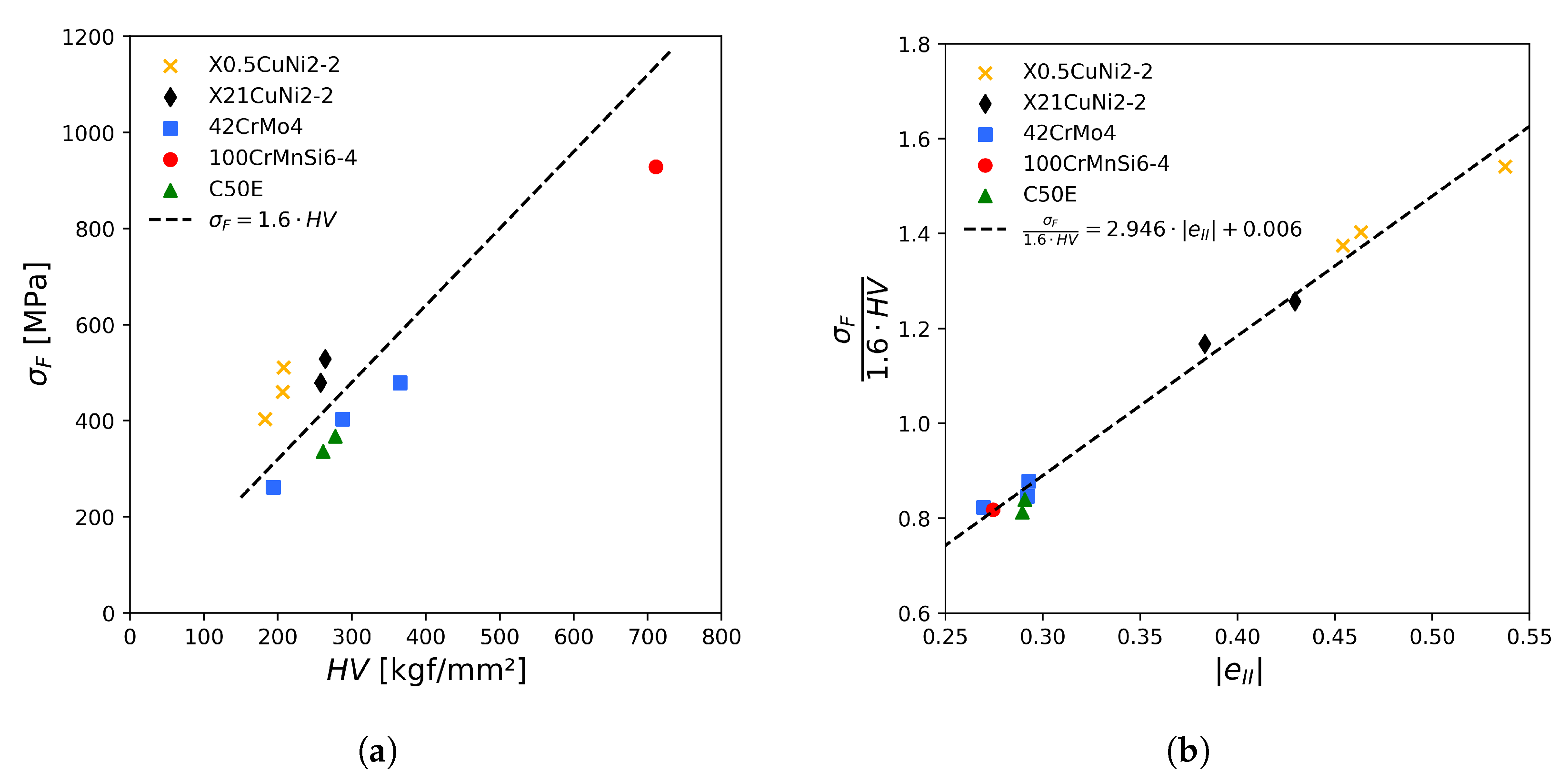
For the investigated materials, σ F deviated from the values predicted by σ F = 1.6 · H V , as shown in Figure 11a. The deviation of the data point for the 100CrMnSi6-4 material may be due to its hardness of approximately 700 kgf/mm2, which is higher than the validity criterion of H V < 400 kgf/mm2 for the relation σ F = 1.6 · H V (see Section 2.5 and estimation 60). Additionally, this estimation was suggested as a rule of thumb for low- and medium-strength steels, and may therefore not be suitable for this particular material (a bearing steel). However, by considering the ratio σ F 1.6 · H V , the deviation of the experimental values from those predicted by the rule of thumb was observed to correlate well with the cyclic hardening exponent e I I (Figure 11b) as
σ F 1.6 · H V = 2.946 · | e I I | + 0.006
Rearranging this equation, the following relation was obtained:
σ F = 4.7136 · | e I I | · H V + 0.0096 · H V
Estimation 92 was established by neglecting the final term of this equation and determining the correlation between σ F and the product of H V and | e I I | by linear regression.

2.9. Estimations Based on Flaw Size

In Table 9, estimations for σ F are presented where the presence of an imperfection is an explicit parameter. It can be noted that during the derivation of estimation 69, the size of material impurities was also taken into account. However, by establishing additional correlations, this parameter was eliminated from the final estimation. It should also be mentioned that while the term “defect” is often used in the literature, the more general terms “flaw” or “imperfection” will be used here instead. In the context of evaluating structural integrity, a “flaw” can only be considered a “defect” after analysis by means of workmanship rules or engineering critical assessment. For clarity, it is worth mentioning that σ and K I will be used to refer to stress amplitudes and mode I stress intensity factor amplitudes, respectively. When expressing ranges of these quantities, a “ Δ ” symbol will be used.
Estimation 93 was originally established by Murakami and Endo [47] based on rotating bending fatigue data for specimens with the following types of artificial surface flaws:
  • Drilled holes with diameters from 40 to 500 µm and depths greater than 40 µm;
  • Notches with depths from 5 to 300 µm;
  • Circumferential cracks with a depth greater than 30 µm;
  • Vickers hardness indentations with a diagonal length of 72 µm.
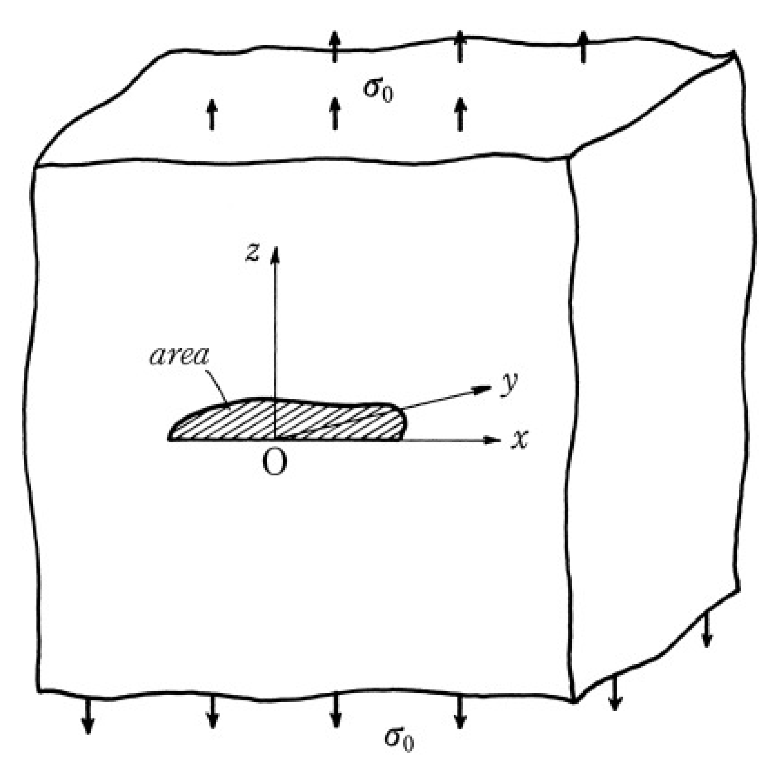
For a surface crack in an infinite body under a remotely applied tension stress σ 0 , the following solution for the stress intensity factor at the maximum stress in a load cycle K I , m a x was considered:
K I , m a x = 0.65 · σ 0 · π · a r e a s
The parameter a r e a s (with unit m in the equation above) was defined as the square root of the area of the projection of the crack onto the plane perpendicular to the direction of the maximum tensile stress, as shown in Figure 12 (the subscript s denotes a surface crack).
By considering the “fatigue limit” as the critical condition for crack propagation, a relation was established with the threshold stress intensity factor range Δ K I , t h . By using µm as the unit for a r e a s , Δ K I , t h was calculated from the experimental data as
Δ K I , t h = 2 · 0.65 · σ F · π · a r e a s · 10 6
For a r e a s 1000 µ m , regardless of the material, the relation between Δ K I , t h and a r e a s was described as
Δ K I , t h ( a r e a s ) 1 / 3
Additionally, Δ K I , t h was related to H V as (with C a constant term independent of the material)
Δ K I , t h ( H V + C )
Combining the two proportionalities resulted in a general relation between Δ K I , t h , H V , and a r e a s :
Δ K I , t h = C 1 · ( H V + C 2 ) · ( a r e a s ) 1 / 3
The coefficients were determined by the least squares method as C 1 = 3.3 · 10 3 and C 2 = 120 . The fatigue strength was then determined as
σ F = Δ K I , t h 2 · 0.65 · π · a r e a s · 10 6 = 1.43 · ( H V + 120 ) ( a r e a s ) 1 / 6
This estimation would predict an infinite fatigue strength for an imperfection-free material. As an upper limit on σ F , the empirical relation of σ F 0.5 · σ U 1.6 · H V was recommended.
When extending the analysis to internal flaws [45], the following expression for K I , m a x was used (with the subscript i denoting an internal flaw):
K I , m a x = 0.5 · σ 0 · π · a r e a i
The following relation between a r e a i and a r e a s to obtain the same K I , m a x was obtained from Equations (21) and (27):
a r e a i = 1.69 · a r e a s
The substitution in Equation (26) resulted in
σ F = 1.56 · ( H V + 120 ) ( a r e a i ) 1 / 6
For an imperfection in contact with the free surface, the following relation was derived through a similar analysis [60] (p. 111) of the stress intensity factors:
σ F = 1.41 · ( H V + 120 ) ( a r e a ) 1 / 6
In [10], Murakami et al. applied estimation 93 to predict the fatigue strength of 34CrMo4 steel specimens with failure initiating at interior inclusions for a fatigue life of around 10 8 cycles. The estimated fatigue strength was reported to be 10% nonconservative compared with the experimental results. Around the inclusion where the fatigue crack had initiated, an optically dark area (ODA) was observed, which was hypothesised to be related to the presence of hydrogen. By including the size of this region in the a r e a parameter, an improved estimation was obtained. However, the size of the ODA cannot be determined prior to the fatigue test [61].
Liu et al. [11,62] performed experiments up to 10 9 cycles on spring and bearing steel alloys and established estimations 94 and 95 based on the following expression:
K I , t h = 1.8 · 10 3 · ( H V + 120 ) · ( a r e a ) 1 / 3
The authors noted that the threshold stress intensity factor K I , t h is better suited to represent the critical condition for crack propagation for R < 0 rather than the threshold stress intensity factor range Δ K I , t h [11]. Estimation 94 was determined based on Equations (27) and (31) [62], analogous to the derivation of Murakami’s estimation above. As ODAs were observed only for fatigue failures beyond 10 6 cycles, it was assumed that the effect of hydrogen did not need to be considered. Therefore, this estimation was put forward as a prediction for the fatigue strength at 10 6 cycles, which was validated with experimental data. In the derivation of estimation 95, the effect of hydrogen on the formation of ODAs was taken into account by introducing an additional stress intensity factor, which allowed for eliminating the requirement of including the area of the ODA in a r e a [61]. This estimation was proposed to determine the fatigue strength at a fatigue life of 10 9 cycles [62].
Estimation 96 was derived by Chapetti et al. [63] on the basis of the following solution for Δ K I for a penny-shaped internal crack (with a in m):
Δ K I = 2 π · Δ σ · π · a
The authors defined “internal fatigue limit” as the “stress below which a crack length of three times the maximum inclusion radius cannot propagate” [63]. Therefore, assuming a = 3 · R i m a x (with R i m a x the maximum inclusion radius in µm), the following expression was obtained from Equation (32):
σ F = 256 · Δ K I , t h R i m a x
To determine Δ K I , t h , Equation (25) was rewritten by substituting a r e a = π · a = π · 3 · R i m a x , resulting in
Δ K I , t h = 4 · 10 3 · ( H V + 120 ) · a 1 / 3 = 4 · 10 3 · ( H V + 120 ) · ( 3 · R i m a x ) 1 / 3
An upper limit of 10 MPa m1/2 was proposed based on data from the literature.
To generalise estimation 93, Murakami [60] (pp. 124–125) suggested to include the effect of a nonzero mean stress by multiplication with the following factor:
1 R 2 α
By analysing the results of rotating bending tests on specimens containing holes with a depth and a diameter of 100 µm, the parameter α was observed to not be strongly dependent on the material. To avoid increasing the complexity of applying the estimation, a correlation with H V was determined. However, it was also noted that insufficient data were available to determine the most appropriate material property to relate with α . If only the mean stress is known, R will depend on σ F as (in case of a mean tensile stress σ m ) [60] (p. 127)
R = σ m σ F σ m + σ F
Therefore, an iterative procedure is required to determine σ F . Estimation 98 was reported to be a suitable simplification to avoid the iterative calculations [60] (p. 129). This estimation was originally developed by regarding the residual stress due to shot peening as the mean stress.
A further modification of Murakami’s estimation (given by estimation 99) was derived by Song and Choi [64] in their research on an induction-hardened steel. Apart from the initial flaw size, the size of nonpropagating short cracks was considered in the determination of Δ K I , t h , resulting in
a r e a t o t a l = a r e a i n i t i a l + a r e a s h o r t c r a c k = κ · a r e a i n i t i a l
Δ K I , t h = α κ C 3 · ( H V + C 2 ) · ( a r e a s ) C 3
Fitting the parameters to experimental data resulted in κ = 1.46 , α = 4.0 · 10 3 , C 2 = 120 , and C 3 = 1 / 3 . Additionally, residual stresses σ r at the surface were incorporated in the form of a modified R-ratio, with the fitting parameter m determined as 0.506
R m o d = σ m i n + m · σ r σ m a x + m · σ r
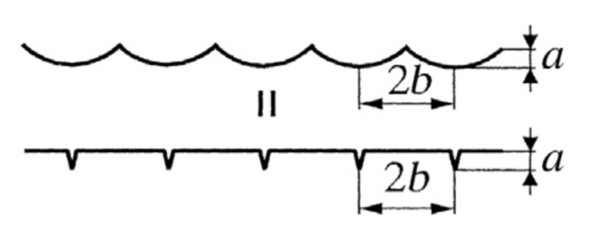
To model the effect of surface roughness on the fatigue strength, Murakami [60] (pp. 407–422) performed experiments on specimens with an artificial, periodic surface roughness. As shown in Figure 13, the pattern of grooves with depth a and pitch b is modelled as a series of notches. For this idealised case, the parameter a r e a R was determined as
a r e a R 2 · b = 2.97 · a 2 · b 3.51 · a 2 · b 2 9.74 · a 2 · b 3 for a 2 · b < 0.195 0.38 for a 2 · b > 0.195
In [65], this estimation was applied to specimens with a random surface finish. The definitions of the parameters a and b are shown in Figure 14. Using the maximum height R y for a resulted in underestimations of the fatigue strength, while the predictions obtained from the average roughness R a showed better agreement with the experimental data.
Estimation 101 was first established by Rigon and Menghetti in [66] for R = 1 and subsequently extended for R = 0 and R = 0.5 in [46]. Both conventionally and additively manufactured metals were considered. The following correlation between the threshold stress intensity factor range Δ K t h , L C , e s t , R and a microstructural length parameter l (in µm) and H V was proposed:
Δ K t h , L C , e s t , R = α R · l β R + γ R · H V δ R
Definitions for l for conventionally manufactured steels are given in Table 10, and the parameters α R , β R , γ R , and δ R are given in Table 11.
The fatigue strength amplitude for imperfection-free material ( Δ σ 0 , e s t , R 2 ) was estimated by generalising estimation 60 by using the Goodman equation:
Δ σ 0 , e s t , R 2 = 3.2 · H V · 1 R 3 R
The length parameter a 0 of the El Haddad–Smith–Topper model was determined as
a 0 , e s t , R = 1 π · Δ K t h , L C , e s t , R Δ σ 0 , e s t , R 2
The fatigue strength was then estimated as
σ F = 0.5 · Δ σ g , t h , e s t , R = 0.5 · Δ σ 0 , e s t , R · a 0 , e s t , R α 2 a r e a + a 0 , e s t , R α 2
The parameter α is 0.65 for a surface flaw and 0.5 for an interior flaw.
Based on his estimation for the S–N curve (described in Section 3.1), Furuya [67] suggested the existence of a plateau in the S–N curves with a knee point at 2 · 10 9 at 1 · 10 10 cycles for, respectively, a r e a = 20 µ m and a r e a = 100 µ m . The fatigue strengths were predicted as
σ F = B 1 · a r e a b 3
The resulting predictions are summarised in estimations 102 to 108. The author did, however, note that fatigue tests up to 10 11 cycles are required to validate whether the predictions are indeed a “fatigue limit” (i.e., a plateau in the S–N curve).
To predict σ F by applying one of the estimations described above, a suitable value for the a r e a must be determined. In [68], a Gaussian distribution was determined based on fracture surface analysis by SEM, from which the average value was used. Murakami [69] proposed applying statistics of extreme values to determine an upper bound for a r e a (and therefore a lower bound for σ F ) based on the investigation of a small volume of material. Further developments of this method can be found in [70].
In the estimations above, the effect of flaws on a material’s fatigue strength was described by a fracture-mechanics-based approach. However, in [71], the volume fraction of nonmetallic inclusions (V) was used to establish estimation 109. The “fatigue strength coefficient” k was defined as
k = σ F · H V 1
Samples of the investigated steel were tempered at five different temperatures. While quadratic relations between k and V were determined for each tempering temperature, estimation 109 presents the relation determined by considering all experimental data.
Table 9. Estimations for fatigue strength σ F based on flaw size.
No.EstimationMaterial aGerman Equivalent (Material Number) b [21]RcTest Type c,dNumber of Cycles cNotesRef.
93 σ F = C · ( H V + 120 ) ( a r e a ) 1 / 6 S10CC10E (1.1121)−1RB 10 7 C = 1.43 for surface flaw[10,45,47,60]
S30CC30 (1.0528) C = 1.56 for interior flaw
S35CC35 (1.0501) C = 1.41 for flaw in contact with surface
S45CC45 (1.0503)
S50CC50 (1.0540)
YUS170/Upper limit: 1.6 · H V = 0.5 · σ U
Maraging steel
70/30 brass
2017-T4 Al 10% nonconservative for 10 8 cycles
94 σ F = 2 · ( H V + 120 ) ( a r e a ) 1 / 6 60Si2Cr
55SiCr6-3 (1.1704)−1R 10 6 For interior flaw[11,62]
60Si2CrV/
60Si2Mn 60Si7 (1.5027)
GCr15VM/
GCr15ER /
95 σ F = 2.7 · ( H V + 120 ) 15 / 16 ( a r e a ) 3 / 16 60Si2CrV/ 1 R 10 9 For interior flaw[61]
SUP1254SiCr6 (1.7102)
60Si2Mn 60Si7 (1.5027)
60Si2Cr55SiCr6-3 (1.1704)
GCr15100Cr6 (1.3505)
NHS1/
40CrNiMo40NiCrMo6 (1.6565)
DIN 50CrV4(1.2241)
DIN 54SiCrV6(1.8152)
DIN 54SiCr6(1.7102)
96 σ F = 256 · Δ K t h R i m a x

Δ K t h = 4 · 10 3 · ( H V + 120 ) · 3 · R i m a x 1 / 3
if Δ K t h 10 MPa m1/2

Δ K t h = 10 MPa m1/2 otherwise
SUJ2100Cr6 (1.3505)/// [63]
SCM43534CrMo4 (1.7220)
SNCM43940NiCrMo6 (1.6565)
97 σ F = C · ( H V + 120 ) ( a r e a ) 1 / 6 · 1 R 2 α

α = 0.226 + H V · 10 4
S10C
Maraging steel
C10E (1.1121)/RB/ C = 1.43 for surface flaw
C = 1.56 for interior flaw
[60]
98 σ F = 1.56 · ( H V + 120 ) a r e a 1 / 6 1 2 · σ m Shot-peened gear steel ///Residual stress regarded as mean local stress[60]
99 σ F = 1.73 · ( H V + 120 ) 1.46 · a r e a 1 / 6 · 1 R m o d 2

R m o d = σ m i n + 0.506 · σ r σ m a x + 0.506 · σ r
SCM44042CrMo4 (1.7225)−1RB 10 7 [64]
100 σ F = 1.43 · ( H V + 120 ) a r e a R 1 / 6

a r e a R 2 · b = 2.97 · a 2 · b 3.51 · a 2 · b 2 9.74 · a 2 · b 3 for a 2 · b < 0.195

a r e a R 2 · b = 0.38 for a 2 · b > 0.195
S45CC45 (1.0503)−1RB 10 7 Idealised surface roughness (dimensions a and b) modelled as surface flaw

Applied to actual surface roughness in [65]
[60]
101 Δ σ 0 , e s t , R 2 = 3.2 · H V · 1 R 3 R

Δ K t h , L C , e s t , R = α R · l β R + γ R · H V δ R

a 0 , e s t , R = 1 π · Δ K t h , L C , e s t , R Δ σ 0 , e s t , R 2

Δ σ g , t h , e s t , R = Δ σ 0 , e s t , R · a 0 , e s t , R α 2 a r e a + a 0 , e s t , R α 2

σ F = 0.5 · Δ σ g , t h , e s t , R
Mild steel −1, 0, 0.5//l: material dependent microstructural length parameter (see Table 10)

α R , β R , γ R , δ R : dependent on R (see Table 11)

α = 0.65 for surface flaws
α = 0.5 for interior flaws
[46,66]
SM41BS235JR (1.0038)
Low-carbon steel
C45(1.0503)
403/410 12%Cr/
17-4 PHX5CrNiCuNb16-4 (1.4542)
300 M41SiNiCrMoV7-6 (1.6928)
Alloy steel
MS/
AISI304X5CrNi18-10 (1.4301)
EA4T/
30Cr2Ni4MoV/
25Cr2Ni2MoV/
SA387-2-2212CrMo9-10 (1.7375)
2.25 Cr - 1 Mo/
CrMoV /
102 σ F = 60.2 · ( a r e a ) 0.22 SCM44042CrMo4 (1.7225)−1RB, UA, US 2 · 10 9 to 1 · 10 10 [67]
103 σ F = 80.4 · ( a r e a ) 0.16 SCM44042CrMo4 (1.7225)0UA 10 4 to 10 10 [67]
104 σ F = 53.4 · ( a r e a ) 0.23 SUP7 (tempered at 430 °C)60Si7 (1.5027)−1RB, UA, US 2 · 10 9 to 1 · 10 10 [67]
105 σ F = 99.4 · ( a r e a ) 0.17 SUP7 (tempered at 500 °C)60Si7 (1.5027)−1RB, UA, US 2 · 10 9 to 1 · 10 10 [67]
106 σ F = 44.5 · ( a r e a ) 0.26 SUJ2100Cr6 (1.3505)−1RB, UA, US 2 · 10 9 to 1 · 10 10 [67]
107 σ F = 53.8 · ( a r e a ) 0.23 SNCM43940NiCrMo6 (1.6565)−1RB, UA, US 2 · 10 9 to 1 · 10 10 [67]
108 σ F = 36.4 · ( a r e a ) 0.26 S40CC40 (1.0511)−1RB, UA, US 2 · 10 9 to 1 · 10 10 [67]
109 k = σ F · H V 1
k = 17.082 · V 2 + 8.0935 · V + 0.1357
Low-carbon steel −1RB 10 7 V: volume% of nonmetallic inclusions[71]
a /: no specific material was provided in the original source; b /: no equivalent material was found; c /: not provided in the original source; d R: resonance; RB: rotating bending; UA: uniaxial; US: ultrasonic.
Table 10. Definition of the microstructural parameter l for estimation 101 [46]. Reproduced with permission from Rigon and Meneghetti, Int. J. Fatigue; published by Elsevier, 2022.
MaterialDefinition of l (in µm)
Ferritic steelsFerritic grain size
Austenitic stainless steelsAustenitic grain size
Pearlitic steelsPearlite colony size
Dual phase (ferritic–martensitic steels)Ferritic grain size (with ferrite percentage higher than 50%)
Martensitic steelsMartensite lath widths (or packet size of martensite laths)
Bainitic steelsBainite packet size
Table 11. Parameters α R , β R , γ R , and δ R for estimation 101 [46]. Reproduced with permission from Rigon and Meneghetti, Int. J. Fatigue; published by Elsevier, 2022.
R α R β R γ R δ R
1 4.50.127 2.29 · 10 2 −0.81
01.820.16553.5−0.52
0.51.680.2035.94−0.26

3. Estimations of the S–N Curve

3.1. Estimations Based on Murakami’s Model

Table 12 lists estimations for the S–N curve, which were derived from Murakami’s work described in Section 2.9. As mentioned in the introduction, the estimations will not be classified according to the material properties on which they are based. Rather, a more chronological structure will be followed to more clearly show the assumptions at the basis of these derivations and the relations between them.
Wang et al. [12] proposed to extend Murakami’s estimation by including the number of cycles to failure, resulting in estimation 110. The constant factor C in Murakami’s estimation was replaced by a factor β :
β = 3.09 0.12 · log N for interior imperfections 2.79 0.108 · log N for surface imperfections
These equations were derived from experimental data of high-strength steel alloys. Applying Murakami’s estimation to the experimental data resulted in an underestimation of the fatigue strength ranging from 21% to 39%, while the modified estimation resulted in errors between 14 % and +5.6%.
In [72], Bandara et al. proposed further modifications to the estimation developed by Wang et al. A first alteration concerned replacing the location-dependent factor β with a single equation, namely,
β = 2.41 0.109 · log N
This equation was determined based on experimental data for 45 different steel alloys extracted from the literature. For R = 1 , substitution in Wang et al.’s estimation resulted in estimation 111. A second simplification concerned eliminating the parameter a r e a . The location dependency was eliminated by averaging the solutions for K I , m a x for surface cracks (Equation (21)) and internal flaws (Equation (27)), resulting in
K I , m a x = 0.575 · σ 0 · π · a r e a
A threshold value for crack propagation was proposed as K I , t h = 1.9 MPa m based on data from experiments at R = 1 . Additionally, a fatigue strength at 10 7 cycles of 0.5 · σ U was assumed. The following approximation of a r e a (in m) resulted from substituting these two values in Equation (49):
a r e a = 14 σ U 2
Substituting the above approximation for a r e a in estimation 111 resulted in estimation 112.
In summary, Wang et al.’s estimation was simplified to a single equation where only H V and σ U were required to estimate the fatigue strength. In case one of these material properties was unknown, using the relation σ U = 3.33 · H V was suggested. After including data for aluminium and magnesium alloys and further analysis of the relation between σ F and σ U 1 / 3 , estimation 113 was determined, where only σ U was required. The authors reported that while the fatigue strengths predicted by estimation 112 were within a ± 20% error margin for 95% of the investigated steels, a larger deviation was observed for materials with σ U > 2000 MPa, σ F > 900 MPa, and carbon equivalency > 1%.
Bandara et al. [20] established estimations 114 and 115 as a more conservative modification of Wang et al.’s model. The derivation of these estimations is analogous to the description above. Instead of approximating a r e a based on an average value for K I , t h , an upper bound was determined based on higher values for K I , t h reported in the literature. As a result, K I , t h was assumed to be equal to 6.0 MPa m . By additionally assuming σ F = 0.5 · σ U at 10 7 cycles, a r e a was approximated as
a r e a = 139 σ U 2
It should be noted that the dataset used to establish this estimation contained both rotating bending experiments and uniaxial experiments. However, the stress distributions in these load cases are not identical, as discussed in Section 2.1.
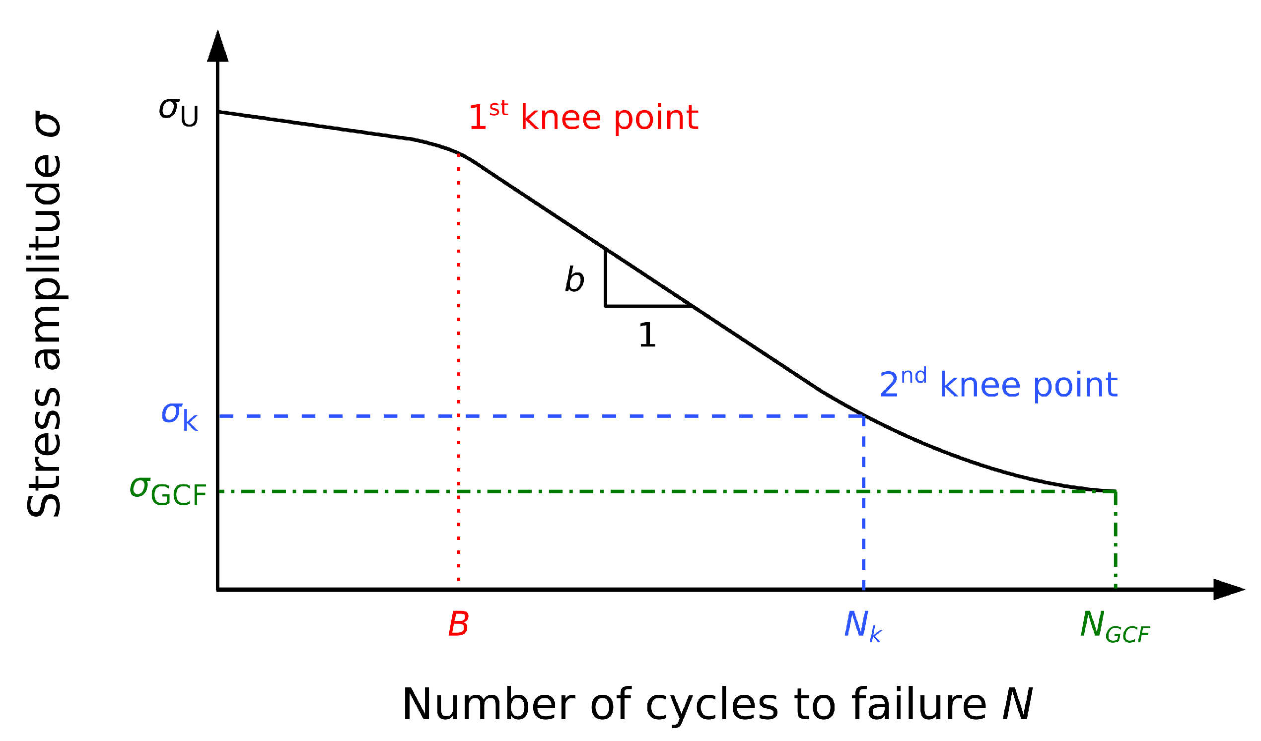
In [73], Bandara et al. used their previously determined estimation 112 as a basis for developing an estimation for a full-range S–N curve (i.e., 1 / 4 < N < 10 10 ) based on the Palmgren function:
σ F = a · ( N + B ) b + c
Figure 15 shows the definitions of the quantities used by Bandara et al. to determine the parameters a, B, and c in Equation (52) by considering three points on the S–N curve, namely, a static load (N = 1/4, σ U ), the second knee point ( N k , σ k ), and a point in the gigacycle regime ( N G C F , σ G C F ). By assuming B 1 / 4 , N k B , and N G C F B , the following solutions were obtained:
a = σ G C F σ k N G C F b N k b
c = 1 2 · ( σ G C F + σ k ) · ( N G C F b N k b ) ( σ G C F σ k ) · ( N G C F b + N k b ) N G C F b N k b = σ k · N G C F b σ G C F · N k b N G C F b N k b
B = σ U c a 1 / b
The authors used estimation 112 to determine σ G C F , recommending N G C F = 10 10 [73] or N G C F = 10 9 [74]. As the second knee point was assumed to exist around 10 6 to 10 7 cycles, the authors assumed σ k = 0.5 · σ U , based on Meggiolaro and Castro’s work in [15]. By again using estimation 112, N k was determined as
N k = 10 0.155 · ( H V + 120 ) · σ U 1 / 3 0.5 · σ U 0.007 · ( H V + 120 ) · σ U 1 / 3
The value for b was determined iteratively by considering the first knee point (B, σ k ) in Equation (52) after substituting Equations (53) to (56). For steels with σ U < 400 MPa , σ k could be estimated as 0.76 · σ U , while for steels with 400 MPa < σ U < 1400 MPa , a value of 0.9 · σ U was considered more appropriate. From their analysis, the authors recommended a global value for b of −0.2.
Due to the various assumptions and empirical relations used during the derivation of this model, the validity is limited to steels with σ U < 1400 MPa (due to the assumption of σ k = 0.5 · σ U ) and H V > 70 kgf / mm 2 (due to the use of Murakami’s model, which was based on data with 70 kgf / mm 2 < H V < 720 kgf / mm 2 ).
As both σ U and H V are required for the application of the model described above, the authors subsequently simplified their model to an estimation based only on hardness. In [74], σ k was estimated as 1.7 · H B (based on σ U = 3.4 · H B ). H V was assumed equal to H B for steels with σ U < 1292 MPa based on the ASTM E140-02 standard [75] and data from Murakami and Endo [47]. The modified equations are given in estimation 117. It should be noted that the authors reported a similar derivation in [76]; however, the equation for N k presented the results in unrealistic values in the order of magnitude of 10 320 .
Based on data from the literature, Chapetti et al. [63,77] determined the following relation between the radius of an inclusion ( R i ), the radius of the optically dark area ( R O D A ), and the number of cycles to failure:
R O D A R i = 0.25 · N 0.125
The authors noted that over 90% of the total fatigue life comprises the formation of the ODA. Therefore, it was assumed that the formation of a crack with a = R O D A can be used to estimate the total number of cycles to failure. Based on Equation (32), estimation 118 was then proposed, where Δ K I , t h should be the lower value of Equation (34) and the following upper limit [77]:
Δ K I , t h = 0.0038 · σ U + 15.5
Estimation 119 was established by Liu et al. [62]. The authors determined the parameters in the Basquin equation (Equation (5)) by assuming the validity of estimations 94 and 95 at N = 10 6 cycles and N = 10 9 cycles, respectively.
Akiniwa et al. [78] developed estimation 120 based on their previous experimental data from [79] and Murakami’s solution for K I , m a x in the presence of an internal crack (Equation (27)). The Paris law was used to describe the fatigue crack propagation rate:
d a d N = C · Δ K I m
The fatigue crack propagation process was divided in three regions, each described by a different set of parameters for the Paris law:
  • Crack initiation at an inclusion with the formation of the ODA;
  • Crack propagation outside the ODA, up to the surface;
  • Surface crack propagation.
The authors assumed that most of the fatigue life in the (very) high-cycle regime was consumed in the first stage. Integrating the Paris law resulted in the following expression:
Δ K I m · N a r e a = 2 C · ( m 2 )
For the calculation of the stress intensity factor range, the authors remarked that “only the tensile part of the applied stress is assumed to be effective” [79], therefore using the following expression (with σ a the stress amplitude):
Δ K I = 0.5 · σ a · π · a r e a
The substitution of this equation into Equation (60) resulted in estimation 120. The parameters C and m were determined as 3.44 · 10 21 and 14.2, respectively. Mayer et al. [68] reported C = 4.86 · 10 21 and n = 14.5 for the same material. The difference in these values was suggested to be related to scatter in the experimental data.
Furuya [67] remarked that estimation 120 overestimates the effect of the inclusion size proposed in the following crack propagation law:
d a r e a d N = C · Δ K · ( a r e a ) α m
After integration, the following equations were derived:
σ F ( N ) = 1 π · D 1 m · N 1 m · ( a r e a ) 1 m 1 2 α
D = 2 1 m · 1 2 + α 1 C · 1 m · 1 2 + α
These equations were simplified to
σ F ( N ) = A 1 · N a 2 · ( a r e a ) a 3
Estimations 121 to 127 represent the resulting S–N curve for the investigated materials. It should be noted that data from rotating bending, uniaxial, and ultrasonic fatigue tests were used. In order to apply this estimation to other materials, the author noted that gigacycle fatigue data are required to fit the parameters.
Table 12. Estimations for the S–N curve based on Murakami’s model.
No.EstimationMaterial aGerman Equivalent (Material Number) b [21]RcTest Type c,dNumber of Cycles cNotesRef.
110 σ F ( N ) = β · ( H V + 120 ) ( a r e a ) 1 / 6 · 1 R 2 α

α = 0.226 + H V · 10 4
42Cr-Mo42CrMo4 (1.7225)−1US 4.5 · 10 5 to 7.12 · 10 8 β = 3.09 0.12 · log N for interior flaws
β = 2.79 0.108 · log N for surface flaws
[12]
Cr-V (60CV2)/
Cr-Si (54SC6)54SiCr6 (1.7102)
Cr-Si (55SC7)55SiCr7 (1.7106)
SUP10M 10M3/
SUP10M 10M6/
SUP9 TM1/
111 σ F ( N ) = ( 2.41 0.109 · log N ) · H V + 120 ( a r e a ) 1 / 6 Medium- and high-strength steels −1/ 10 6 to 10 10 [72]
112 σ F ( N ) = 0.001 · ( H V + 120 ) · ( 155 7 · log N ) · σ U 1 / 3 Medium- and high-strength steels −1/ 10 6 to 10 10 Suitable for σ F < 1000 MPa [20][72]
113 σ F ( N ) = 0.707 · σ U 1.214 log N Medium- and high-strength steels
(+Al and Mg alloys)
−1/ 10 6 to 10 10 [72]
114 σ F ( N ) = ( 188 8.5 · log N ) · H V + 120 1000 · H V 1 / 3 · 1 R 2 α CrMo −1RB, UA 10 6 to 10 10 [20]
Cr
CrSi
SiMn
SiCr
SiCrV
NiCrMo
CrV
MnSiCr
CrMn
CrNiMo
SUP10M51CrV4 (1.8159)
SUJ2100Cr6 (1.3505)
Aermet100/
SUP1254SiCr6 (1.7102)
NSH1/
GRV/
GVM/
KSFA/
D38MSV5S/
AISI8620/
C steels
115 σ F ( N ) = ( 106 4.8 · log N ) · H V + 120 1000 · σ U 1 / 3 · 1 R 2 α See estimation 114 −1RB, UA 10 6 to 10 10 [20]
116 σ F ( N ) = a · ( N + B ) b + c

a = σ G C F σ k N G C F b N k b

c = σ k · N G C F b σ G C F · N k b N G C F b N k b

B = σ U c a 1 / b

N k = 10 0.155 · ( H V + 120 ) · σ U 1 / 3 0.5 · σ U 0.007 · ( H V + 120 ) · σ U 1 / 3

σ k = 0.5 · σ U

σ G C F = 0.001 · ( H V + 120 ) · ( 155 7 · log N G C F ) · σ U 1 / 3
/ −1/ 1 / 4 to 10 10 b = 0.2
N G C F = 10 9 or 10 10
Valid for 240 MPa < σ U < 1400 MPa
[73]
117 σ F ( N ) = a · ( N + B ) b + c

a = σ G C F σ k N G C F b N k b

c = σ k · N G C F b σ G C F · N k b N G C F b N k b

B = 3.4 · σ U c a 1 / b

N k = 10 0.233 · ( H B + 120 ) · H B 1 / 3 1.7 · H B 0.0105 · ( H B + 120 ) · H B 1 / 3

σ k = 1.7 · H B

σ G C F = 0.138 · H B 1 / 3 · ( H B + 120 )
/ −1/ 1 / 4 to 10 10 b = 0.2
N G C F = 10 9 or 10 10
Valid for σ U < 1292 MPa
[74]
118 σ F ( N ) = 444 · Δ K t h 0.25 · N 0.125 · R i

Δ K t h : lower value of

4 · 10 3 · ( H V + 120 ) · ( 0.25 · N 0.125 · R i ) 1 / 3

or

0.0038 · σ U + 15.5
SUJ2100Cr6 (1.3505)−1RB, UA, US 10 5 to 10 9 Additional correlation: σ U = 3.28 · H V [63,77]
SCM435 34CrMo4 (1.7220)
SNCM43940NiCrMo6 (1.6565)
119 σ F ( N ) = σ f · ( 2 · N ) b

b = 1 3 · log [ 1.35 · ( H V + 120 ) 1 / 16 · ( a r e a ) 1 / 48 ]

σ f = 1.12 · ( H V + 120 ) 9 / 8 ( a r e a ) 1 / 8
60Si2Mn60Si7 (1.5027)−1US > 10 6 [62]
60Si2CrV/
54SiCr6(1.7102)
120 σ F ( N ) = 2 π · 2 C ( m 2 ) 1 / m · ( a r e a ) 1 / m 1 / 2 · N 1 / m SUJ2100Cr6 (1.3505)−1US > 10 7 C = 3.44 · 10 21
m = 14.2
[78]
121 σ F ( N ) = 292.2 · N 0.049 · ( a r e a ) 0.171 SCM44042CrMo4 (1.7225)−1RB, UA, US 10 4 to 10 10 [67]
122 σ F ( N ) = 443.8 · N 0.053 · ( a r e a ) 0.107 SCM44042CrMo4 (1.7225)0UA 10 4 to 10 10 [67]
123 σ F ( N ) = 175.9 · N 0.037 · ( a r e a ) 0.193 SUP7 (tempered at 430 °C)60Si7 (1.5027)−1RB, UA, US 10 4 to 10 10 [67]
124 σ F ( N ) = 237.4 · N 0.027 · ( a r e a ) 0.143 SUP7 (tempered at 500 °C)60Si7 (1.5027)−1RB, UA, US 10 4 to 10 10 [67]
125 σ F ( N ) = 216.1 · N 0.049 · ( a r e a ) 0.211 SUJ2100Cr6 (1.3505)−1RB, UA, US 10 4 to 10 10 [67]
126 σ F ( N ) = 360.3 · N 0.059 · ( a r e a ) 0.171 SNCM43940NiCrMo6 (1.6565)−1RB, UA, US 10 4 to 10 10 [67]
127 σ F ( N ) = 370.8 · N 0.072 · ( a r e a ) 0.188 S40CC40 (1.0511)−1RB, UA, US 10 4 to 10 10 [67]
128 σ F ( N ) = C 1 / n ( a r e a ) 1 / 6 · N 1 / n 100Cr6(1.3505)−1US 10 5 to 10 9 C = 6.47 · 10 98
n = 28.82
[68]
129 d a d N = 10 4 · σ F σ M u r a k a m i 1 2.0 · a S35CC35 (1.0501) 1 RB, UA 10 4 to 10 7 σ M u r a k a m i : from estimation 93
For steels with H V > 450 kgf / mm 2 : reduce σ M u r a k a m i by 20%
Numerical integration required to determine fatigue life (final crack size: 1.0 or 2.0 mm)
[80]
S45CC45 (1.0503)
Maraging steel
Ductile cast iron FCD400
AM Ti-4Al-6V
AM Inconel 718
a /: no specific material was provided in the original source; b /: no equivalent material was found; c /: not provided in the original source; d RB: rotating bending; UA: uniaxial; US: ultrasonic.
Mayer et al. [68] performed experiments to determine the S–N curve for 100Cr6 bearing steel. The authors remarked that a significant reduction in scatter in the S–N data could be achieved when normalising the applied stress amplitude ( σ ) with the fatigue strength predicted by Murakami’s model ( σ M u r a k a m i ), i.e.,
σ σ M u r a k a m i = σ · ( a r e a ) 1 / 6 1.56 · ( H V + 120 )
A linear relation between this normalised ratio and N was determined in a double logarithmic diagram, resulting in estimation 128.
Estimation 129 was established by Murakami and Endo in [80]. To predict the fatigue life at a given stress amplitude σ F , the following equation was proposed:
d a d N = C * · σ F σ M u r a k a m i 1 m * · a n *
In this equation, σ M u r a k a m i is given by estimation 93. After determining the parameters C * , m * , and n * from experimental data for carbon steel C45 and additively manufactured (AM) Ti-4Al-6V, the authors noted that the values C * = 10 4 , m * = 2.0 , and n * = 1 were suited for both materials. Therefore, they suggested to use these values regardless of the specific material if no experimental data were available to determine the actual values. This assumption was validated for C35 steel, maraging steel, ductile cast iron, and AM Inconel 718. Additionally, the model was determined to be suitable to describe both rotating bending and uniaxial tension–compression data. As in their previous work (for instance, [47]), the crack size a was defined as a r e a (in µm). The authors noted that numerical integration is required to determine the number of cycles to failure from Equation (67). To solve this integral, initial and final values for a are required. For the former, statistics of extreme values could be applied as described in Section 2.9. For the latter, the authors suggested a value of a = 1.0 mm or a = 2.0 mm, noting that the fatigue life remaining after a = 1.0 mm is negligibly short. For steels with H V > 450 kgf / mm 2 , the authors recommended reducing the value of σ M u r a k a m i by 20% to improve the accuracy of the prediction.

3.2. Other Estimations

Table 13 presents the remaining number of estimations for the S–N curve, which were not based on Murakami’s model.
In [81], the S–N curve was described by the following equation (similar to the Basquin Equation (5)):
σ F ( N ) = 10 C · N b
To determine the parameters C and b, the following correlations were used to define two points on the S–N curve, resulting in estimation 130:
σ F ( 10 3 ) = 0.9 · σ U
σ F ( 10 6 ) = 0.5 · σ U
A similar model was proposed in [82] based on the following equation:
σ F ( N ) = σ U · N m
To determine the exponent m, the authors recommended estimating the fatigue strength at 10 6 cycles as 0.5 · σ U , resulting in estimation 131.
Estimation 132 was developed based on data for 52 different steel alloys [83]. Similar to the previous estimation, the parameters in the equation describing the S–N curve were determined by considering two points. The first point was defined as ( N σ Y , 0.9 · σ Y ), while the second point was determined by the fatigue strength at 10 6 cycles (for which one of the correlations in Section 2 could be used). It should be noted that the expressions for A and m given in Table 13 were modified from the equations in [83]. The original expression for m returns positive values, therefore resulting in an unrealistic S–N curve where N increases with σ F .
Mukoyama et al. [48] analysed data for various structural carbon steels published by the Society of Materials Science, Japan (JSMS). The S–N curves were assumed to reach a plateau around 10 6 to 10 7 cycles. The sloped part of the S–N curve was described by the following expression:
σ F ( N ) = A · log N + B
The parameters A and B were correlated with the fatigue strength at 10 4 cycles, which in turn was correlated with σ U . As presented in estimations 133 to 135, these correlations were established for three different material groups. For the materials S45C and S50C, data for material that underwent a quench and temper process (quenching after heating to 1123 K and tempering after reheating to at least 723 K) or a normalising process were grouped and are denoted by “(Q&T)”. Data for S45C and S50C that underwent different heat treatment procedures were grouped and denoted by “(EQT)”. The authors concluded that the slope A showed good agreement with the experimental data, while the accuracy of the prediction for B was lower.
While the majority of the estimations for the S–N curve described in this section and Section 3.2 were based on an assumed equation describing the S–N curve, Stepanskiy [84] followed an energy-based approach to determine estimations 136 and 137. The full derivation can be found in [84]; only the main equations and assumptions will be presented here. Fatigue failure was assumed to occur when the plastically dissipated energy due to tensile stresses reached a threshold value (denoted as [ W ] ), determined by the true stress and strain during a static tensile test:
[ W ] = 0 ( ϵ t r ) f σ t r d ϵ t r
The authors noted that the following approximation may be used for [ W ] :
[ W ] 0.25 · σ Y + 3 · σ U 1 ψ n · ln 1 1 ψ n + 0.2 · σ U · 1 1 ψ n + 4 1 ψ · ln 1 ψ n 1 ψ
In Equations (73) and (74), the following symbols were used:
  • ( ϵ t r ) f : true strain at failure;
  • σ t r : true stress;
  • ϵ t r : true strain;
  • ψ : reduction in area after failure;
  • ψ n : reduction in area at the onset of necking.
Estimation 136 was determined by assuming a uniaxial load and integrating the equivalent plastic stress and strain over the total number of fatigue cycles. A distinction was made between materials with body-centred cubic, face-centred cubic, or hexagonal close-packed crystal lattice structures. For R > 0 , estimation 137 was derived.
While all material parameters required for the application of estimations 136 and 137 can be determined from static tensile tests, it is worth noting that a specific instrumentation is required to measure the reduction in area throughout the experiment.

4. Suggestions for Future Research

Based on the previous sections, it is clear that estimating the fatigue strength (in terms of an entire S–N curve and/or the fatigue strength at a given fatigue life) of steels has received a significant amount of research interest.
A large number of estimations for fatigue strength have been established over the years. Rather than providing additional predictions to the state of the art, there should be increased focus on the verification and comparison of existing models with a wide range of experimental datasets. Most researchers have often based their analysis on a limited dataset for a few specific materials. A critical evaluation of different estimations using a larger variety of materials will be beneficial to judge whether the applicability of these predictions can be extended. For instance, Li et al. [14] performed such analysis, comparing different predictions for the fatigue strength at 10 6 cycles for 117 different steels. A second example is Meggiolaro and Castro’s work [15], which was based on an extensive dataset consisting of 724 different steels. Compiling the various available raw datasets published in the literature into a single database would be a substantial step towards a wide verification of different predictions. Unfortunately, experimental data are often reported in graphic form only (e.g., S–N curves), which hinders the use by other researchers. Providing numerical data in tabulated form, for example, in an appendix or ideally in a machine-readable file format, is also essential for a collaborative research effort. In addition, material names are often stated according to various national naming conventions. The authors intended to set a precedent for reporting standards by using equivalent names and material numbers in the previous sections.
Similar observations and recommendations were stated in a review on nonlinear fatigue damage accumulation models [85]. As a follow-up to that review, a comprehensive and reliable database comprising high-quality data of fatigue block loading experiments was developed [86] and published as an open-access repository [87]. The development of such open-access dataset with fatigue test data and related mechanical properties is considered crucial to make a significant step forward in verifying and comparing fatigue strength predictions.
It can be remarked that σ U and hardness are the most often used properties from which the fatigue strength is estimated. A further potential research topic may consist of an analysis of a large dataset (similar to the recommendation above), but considering additional material properties such as Charpy impact energy or combinations of multiple properties (e.g., considering metrics for both strength and ductility). To this end, machine learning tools might be a promising alternative to the linear regression method that is often used (as evident from the previous sections). Machine learning tools have been widely applied in the field of materials science during the last few years. The powerful fitting and predictive capabilities of machine learning tools allow for developing relationships between influencing factors (in this case, mechanical properties) and target variables (in this case, fatigue strength properties). For example, He et al. [88] employed artificial neural networks to predict the S–N curve based on chemical composition and monotonic tensile properties. While not directly correlating fatigue strength with other mechanical properties, Agrawal and Choudhary [89] and Liu et al. [90] developed machine learning tools based on data from the Japanese National Institute for Materials Science in order to predict fatigue strength based on chemical composition and material processing parameters (e.g., tempering temperature). During the development of such machine learning model, the quality and quantity of training data are of critical importance. Therefore, compiling an extensive dataset as described above would also constitute a significant contribution in enabling the use of machine learning tools to predict fatigue strength based on (multiple) other mechanical properties.

5. Conclusions

An overview of estimations for the high-cycle fatigue strength of conventionally manufactured steels based on other material properties has been presented. The most important details regarding their applicability were summarised in several tables to provide a well-structured synopsis. While it cannot be guaranteed that all such estimations were included, correlations were provided based on a range of material properties and for a variety of steel alloys and loading conditions.
As a general remark to conclude this review paper, it is perhaps worth reflecting on the methods employed to establish the estimations provided in the previous sections. Researchers have often determined correlations by (linear) regression on a dataset obtained from own experiments, the literature, or a combination of both. However, in the latter two approaches, care must be taken to ensure that only datasets established under identical conditions are combined (e.g., data from uniaxial and rotating bending tests should not be combined). It is therefore critical to report all experimental details when presenting results in order to facilitate the use of these data by other researchers. Additional caution is required when establishing relations based on multiple properties. While the resulting correlation may be considered “good” from a statistical point of view (e.g., a high value for the coefficient of determination R 2 ), the physical interpretation must still be valid.

Funding

This research was funded by Ghent University’s Special Research Fund, grant number BOF/24J/2021/261.

Conflicts of Interest

The authors declare no conflicts of interest.

Abbreviations

The table below lists the most frequently recurring physical quantities together with their symbols and units used in this paper (unless explicitly stated otherwise). It is important to note that all fatigue strengths presented in the tables in this review are stress amplitudes. Stress ranges and stress intensity factor ranges are always denoted by a “Δ” symbol.
SymbolPhysical QuantityUnit
σ F fatigue strength (stress amplitude)MPa
Δ σ stress rangeMPa
Nnumber of cycles-
Rstress ratio-
σ U ultimate tensile strengthMPa
σ Y yield strengthMPa
σ C Y cyclic yield strengthMPa
ψ reduction in area-
H V Vickers hardnesskgf/mm2
H B Brinell hardnesskgf/mm2
H R Rockwell hardness (on different scales)-
a r e a flaw sizeµm
K I , t h mode I threshold stress intensity factorMPa m
Δ K I , t h mode I threshold stress intensity factor rangeMPa m
K I , m a x mode I stress intensity factor at the maximum load in a load cycleMPa m

References

  1. Findlay, S.J.; Harrison, N.D. Why aircraft fail. Mater. Today 2002, 5, 18–25. [Google Scholar] [CrossRef]
  2. Dieter, G.E., Jr. Mechanical Metallurgy; McGraw-Hill Book Company, Inc.: New York, NY, USA, 1961; ISBN 07-016890-3. [Google Scholar]
  3. Das, A.K. Metallurgy of Failure Analysis; The McGraw-Hill Companies, Inc.: New York, NY, USA, 1997; ISBN 0-07-015804-5. [Google Scholar]
  4. Stephens, R.; Fatemi, A.; Stephens, R.; Fuchs, H. Metal Fatigue in Engineering; A Wiley-Interscience Publication, Wiley: Hoboken, NJ, USA, 2000; ISBN 978-0-471-51059-8. [Google Scholar]
  5. Gagg, C.R.; Lewis, P.R. In-service fatigue failure of engineered products and structures—Case study review. Eng. Fail. Anal. 2009, 16, 1775–1793. [Google Scholar] [CrossRef]
  6. Forschungskuratorium Maschinenbau. FKM Guideline: Analytical Strength Assessment; VDMA Verlag: Frankfurt, Germany, 2003; ISBN 3816304257. [Google Scholar]
  7. Schütz, W. A history of fatigue. Eng. Fract. Mech. 1996, 54, 263–300. [Google Scholar] [CrossRef]
  8. ISO 1143:2021; Metallic Materials-Rotating Bar Bending Fatigue Testing. ISO: Geneva, Switzerland, 2021.
  9. Fernández-Canteli, A.; Blasón, S.; Pyttel, B.; Muniz-Calvente, M.; Castillo, E. Considerations about the existence or non-existence of the fatigue limit: Implications on practical design. Int. J. Fract. 2020, 223, 189–196. [Google Scholar] [CrossRef]
  10. Murakami, Y.; Nomoto, T.; Ueda, T. Factors influencing the mechanism of superlong fatigue failure in steels. Fatigue Fract. Eng. Mater. Struct. 1999, 22, 581–590. [Google Scholar] [CrossRef]
  11. Liu, Y.B.; Yang, Z.G.; Li, Y.D.; Chen, S.M.; Li, S.X.; Hui, W.J.; Weng, Y.Q. On the formation of GBF of high-strength steels in the very high cycle fatigue regime. Mater. Sci. Eng. A 2008, 497, 408–415. [Google Scholar] [CrossRef]
  12. Wang, Q.Y.; Berard, J.Y.; Dubarre, A.; Baudry, G.; Rathery, S.; Bathias, C. Gigacycle fatigue of ferrous alloys. Fatigue Fract. Eng. Mater. Struct. 1999, 22, 667–672. [Google Scholar] [CrossRef]
  13. ISO 12107:2012; Metallic Materials-Fatigue Testing-Statistical Planning and Analysis of Data. ISO: Geneva, Switzerland, 2012.
  14. Li, J.; Qiu, Y.Y.; Wang, H.D.; Wang, Z.X. Evaluation of the methods for estimating the fully reversed unnotched fatigue limits of steels. Adv. Mater. Sci. Eng. 2019, 2019, 4098623. [Google Scholar] [CrossRef]
  15. Meggiolaro, M.A.; Castro, J.T. Statistical evaluation of strain-life fatigue crack initiation predictions. Int. J. Fatigue 2004, 26, 463–476. [Google Scholar] [CrossRef]
  16. Harun, M.F.; Mohammad, R. Fatigue properties of JIS H3300 C1220 copper for strain life prediction. AIP Conf. Proc. 2018, 1958, 020001. [Google Scholar] [CrossRef]
  17. Troshchenko, V.T.; Khamaza, L.A. Strain-life curves of steels and methods for determining the curve parameters. Part 1. Conventional methods. Strength Mater. 2010, 42, 647–659. [Google Scholar] [CrossRef]
  18. Tridello, A.; Niutta, C.B.; Rossetto, M.; Berto, F.; Paolino, D.S. Statistical models for estimating the fatigue life, the stress–life relation, and the P–S–N curves of metallic materials in Very High Cycle Fatigue: A review. Fatigue Fract. Eng. Mater. Struct. 2022, 45, 332–370. [Google Scholar] [CrossRef]
  19. Pang, J.C.; Li, S.X.; Wang, Z.G.; Zhang, Z.F. Relations between fatigue strength and other mechanical properties of metallic materials. Fatigue Fract. Eng. Mater. Struct. 2014, 37, 958–976. [Google Scholar] [CrossRef]
  20. Bandara, C.S.; Siriwardane, S.C.; Dissanayake, U.I.; Dissanayake, R. Fatigue failure predictions for steels in the very high cycle region—A review and recommendations. Eng. Fail. Anal. 2014, 45, 421–435. [Google Scholar] [CrossRef]
  21. Verlag Stahlschlüssel Wegst GmbH. Online::Stahlschluessel—Key to Steel. 2023. Available online: https://www.online.stahlschluessel.de/ (accessed on 17 February 2023).
  22. Tóth, L.; Yarema, S.Y. Formation of the science of fatigue of metals. Part I. 1825–1870. Transl. Fiz.-Khimichna Mekhanika Mater. 2006, 42, 87–94. [Google Scholar] [CrossRef]
  23. Socie, D.F.; Mitchell, M.R.; Caulfield, E.M. Fundamentals of Modern Fatigue Analysis. 1978. Available online: https://fcp.mechse.illinois.edu/fcp_report026/ (accessed on 16 May 2023).
  24. Roessle, M.L.; Fatemi, A. Strain-controlled fatigue properties of steels and some simple approximations. Int. J. Fatigue 2000, 22, 495–511. [Google Scholar] [CrossRef]
  25. Andersson, H. Metal Fatigue Principles and Analyses. 2021. Available online: http://www.diva-portal.org/smash/record.jsf?pid=diva2%3A1612930&dswid=-1298 (accessed on 16 May 2023).
  26. Furuya, Y.; Matsuoka, S. Improvement of Gigacycle Fatigue Properties by Modified Ausforming in 1600 and 2000 MPA-Class Low-Alloy Steels. Metall. Mater. Trans. A 2022, 33A, 3421–3431. [Google Scholar] [CrossRef]
  27. Furuya, Y.; Nishikawa, H.; Hirukawa, H.; Nagashima, N.; Takeuchi, E. Catalogue of NIMS fatigue data sheets. Sci. Technol. Adv. Mater. 2019, 20, 1055–1072. [Google Scholar] [CrossRef]
  28. Nishijima, S. Basic Fatigue Properties of JIS Steels for Machine Structural Use NRIM Special Report. 1993. Available online: https://mdr.nims.go.jp/concern/publications/h989r3289 (accessed on 24 January 2023).
  29. Yamaguchi, K.; Abe, T.; Kobayashi, K.; Takeuchi, E.; Hirukawa, H.; Maeda, Y.; Nagashima, N.; Hayakawa, M.; Furuya, Y.; Shimodaira, M.; et al. Gigacycle fatigue data sheets for advanced engineering materials. Sci. Technol. Adv. Mater. 2007, 8, 545–551. [Google Scholar] [CrossRef]
  30. Zhao, A.; Xie, J.; Sun, C.; Lei, Z.; Hong, Y. Effects of strength level and loading frequency on very-high-cycle fatigue behavior for a bearing steel. Int. J. Fatigue 2012, 38, 46–56. [Google Scholar] [CrossRef]
  31. Park, S.H.; Lee, C.S. Relationship between mechanical properties and high-cycle fatigue strength of medium-carbon steels. Mater. Sci. Eng. A 2017, 690, 185–194. [Google Scholar] [CrossRef]
  32. Sperle, J.O. Fatigue strength of high strength dual-phase steel sheet. Int. J. Fatigue 1985, 7, 79–86. [Google Scholar] [CrossRef]
  33. Krumes, D.; Haračić, N.; Vitez, I.; Budi, I. Contribution to the Correlation between Fatigue Endurance and Tensile Strength of Steel. 2000. Available online: https://www.researchgate.net/publication/236942405_Contribution_to_the_correlation_between_fatigue_endurance_and_tensile_strength_of_steel (accessed on 27 January 2023).
  34. Pang, J.C.; Li, S.X.; Wang, Z.G.; Zhang, Z.F. General relation between tensile strength and fatigue strength of metallic materials. Mater. Sci. Eng. A 2013, 564, 331–341. [Google Scholar] [CrossRef]
  35. Savu, V.A.; Mourelatos, Z. Long Life Axial Fatigue Strength Models for Ferrous Powder Metals. SAE Int. J. Mater. Manuf. 2018, 11, 467–479. [Google Scholar] [CrossRef]
  36. Das, B.; Singh, A.; Arora, K.S.; Shome, M.; Paul, S.K. Influence of pre-straining path on high cycle fatigue performance of DP 600 steel. Int. J. Fatigue 2019, 126, 369–380. [Google Scholar] [CrossRef]
  37. Paul, S.K. Correlation between endurance limit and cyclic yield stress determined from low cycle fatigue test. Materialia 2020, 11, 100695. [Google Scholar] [CrossRef]
  38. Zhang, D.; Du, L.; Lan, L.; Gao, C.; Xiao, B. Correlation of Microstructure and Fatigue Properties of Hot-Rolled Steel Strips for Automobile Structural Application. J. Mater. Eng. Perform. 2020, 29, 4009–4017. [Google Scholar] [CrossRef]
  39. Liu, R.; Zhang, P.; Zhang, Z.J.; Wang, B.; Zhang, Z.F. A practical model for efficient anti-fatigue design and selection of metallic materials: I. Model building and fatigue strength prediction. J. Mater. Sci. Technol. 2021, 70, 233–249. [Google Scholar] [CrossRef]
  40. Sperle, J.O.; Nilsson, T. The Application of High Strength Steels for Fatigue Loaded Structures. 1992. Available online: https://www.researchgate.net/publication/285897692_The_application_of_high_strength_steels_for_fatigue_loaded_structures (accessed on 31 January 2023).
  41. Sperle, J.O.; Trogen, H. Influence of yield ratio on the fatigue strength of steel sheet. Scand. J. Metall. 1989, 18, 147–154. [Google Scholar]
  42. Yang, M.; Gao, C.; Pang, J.; Li, S.; Hu, D.; Li, X.; Zhang, Z. High-Cycle Fatigue Behavior and Fatigue Strength Prediction of Differently Heat-Treated 35CrMo Steels. Metals 2022, 12, 688. [Google Scholar] [CrossRef]
  43. Li, J.; Sun, Q.; Zhang, Z.-P.; Li, C.-W.; Qiao, Y.-J. Theoretical estimation to the cyclic yield strength and fatigue limit for alloy steels. Mech. Res. Commun. 2009, 36, 316–321. [Google Scholar] [CrossRef]
  44. Hales, R.; Holdsworth, S.R.; O’Donnell, M.P.; Perrin, I.J.; Skelton, R.P. A Code of Practice for the determination of cyclic stress-strain data. Mater. High Temp. 2002, 19, 165–185. [Google Scholar] [CrossRef]
  45. Murakami, Y.; Kodama, S.; Konuma, S. Quantitative evaluation of effects of non-metallic inclusions on fatigue strength of high strength steels. I: Basic fatigue mechanism and evaluation of correlation between the fatigue fracture stress and the size and location of non-metallic inclusions. Int. J. Fatigue 1989, 11, 291–298. [Google Scholar] [CrossRef]
  46. Rigon, D.; Meneghetti, G. Engineering estimation of the fatigue limit of wrought and defective additively manufactured metals for different load ratios. Int. J. Fatigue 2022, 154, 106530. [Google Scholar] [CrossRef]
  47. Murakami, Y.; Endo, M. Effects of Hardness and Crack Geometries on ΔKth of Small Cracks Emanating from Small Defects. In The Behaviour of Short Fatigue Cracks, EGF Pub. 1; Miller, K.J., de los Rios, E.R., Eds.; Mechanical Engineering Publications: London, UK, 1986; pp. 275–293. [Google Scholar]
  48. Mukoyama, K.; Hanaki, K.; Okada, K.; Sakaida, A.; Sugeta, A.; Nishikawa, I.; Ueno, A.; Sakai, T. A study on estimation of S–N curves for structural steels based on their static mechanical properties. Adv. Mater. Res. 2014, 891–892, 1639–1644. [Google Scholar] [CrossRef]
  49. Mortezaei, S.; Mashreghi, A.R. The Effect of Interaction Between Hardness, Inclusion and Microstructures on the Fatigue Behavior of Steel. J. Metall. Mater. Eng. 2017, 28, 23–36. [Google Scholar]
  50. Gao, C.; Yang, M.Q.; Pang, J.C.; Li, S.X.; Zou, M.D.; Li, X.W.; Zhang, Z.F. Abnormal relation between tensile and fatigue strengths for a high-strength low-alloy steel. Mater. Sci. Eng. A 2022, 832, 142418. [Google Scholar] [CrossRef]
  51. Saruki, K.; Hotta, S.; Fujita, H.; Arai, T. Fatigue strength of steels with thin hard coating. Thin Solid Films 1989, 181, 395. [Google Scholar] [CrossRef]
  52. Hotta, S.; Saruki, K.; Arai, T. Endurance limit of thin hard-coated steels in bending fatigue. Surf. Coat. Technol. 1994, 70, 121–129. [Google Scholar] [CrossRef]
  53. McKelvey, S.A.; Lee, Y.L.; Barkey, M.E. Stress-based uniaxial fatigue analysis using methods described in FKM-guideline. J. Fail. Anal. Prev. 2012, 12, 445–484. [Google Scholar] [CrossRef]
  54. Li, Z.; Wang, Q.; Luo, A.A.; Fu, P.; Peng, L. Fatigue strength dependence on the ultimate tensile strength and hardness in magnesium alloys. Int. J. Fatigue 2015, 80, 468–476. [Google Scholar] [CrossRef]
  55. Martínez, A.; Jaimes, A.; Serna, A.; Uribe, I. Development of a correlation to estimate the fatigue strength for steels based on low-cost tests. Ciencia Tecnología y Futuro 2010, 4, 71–81. [Google Scholar] [CrossRef]
  56. Hassan, A.D. A new prediction of the fatigue limit based on Brinell hardness and ultimate strength for high strength steels. Int. J. Energy Environ. 2018, 9, 77–84. [Google Scholar]
  57. Görzen, D.; Ostermayer, P.; Lehner, P.; Blinn, B.; Eifler, D.; Beck, T. A New Approach to Estimate the Fatigue Limit of Steels Based on Conventional and Cyclic Indentation Testing. Metals 2022, 12, 1066. [Google Scholar] [CrossRef]
  58. Schwich, H.; Görzen, D.; Blinn, B.; Beck, T.; Bleck, W. Characterization of the precipitation behavior and resulting mechanical properties of copper-alloyed ferritic steel. Mater. Sci. Eng. A 2020, 772, 138807. [Google Scholar] [CrossRef]
  59. Görzen, D.; Schwich, H.; Blinn, B.; Bleck, W.; Beck, T. Influence of different precipitation states of Cu on the quasi-static and cyclic deformation behavior of Cu alloyed steels with different carbon contents. Int. J. Fatigue 2020, 136, 105587. [Google Scholar] [CrossRef]
  60. Murakami, Y. Metal Fatigue: Effects of Small Defects and Nonmetallic Inclusions; Elsevier: Amsterdam, The Netherlands, 2019; pp. 1–758. [Google Scholar] [CrossRef]
  61. Liu, Y.B.; Yang, Z.G.; Li, Y.D.; Chen, S.M.; Li, S.X.; Hui, W.J.; Weng, Y.Q. Dependence of fatigue strength on inclusion size for high-strength steels in very high cycle fatigue regime. Mater. Sci. Eng. A 2009, 517, 180–184. [Google Scholar] [CrossRef]
  62. Liu, Y.B.; Li, Y.D.; Li, S.X.; Yang, Z.G.; Chen, S.M.; Hui, W.J.; Weng, Y.Q. Prediction of the S–N curves of high-strength steels in the very high cycle fatigue regime. Int. J. Fatigue 2010, 32, 1351–1357. [Google Scholar] [CrossRef]
  63. Chapetti, M.D.; Tagawa, T.; Miyata, T. Ultra-long cycle fatigue of high-strength carbon steels part II: Estimation of fatigue limit for failure from internal inclusions. Mater. Sci. Eng. A 2003, 356, 236–244. [Google Scholar] [CrossRef]
  64. Song, S.H.; Choi, B.H. Fatigue characteristics and fatigue limit prediction of an induction case hardened Cr-Mo steel alloy. Mater. Sci. Eng. A 2003, 361, 15–22. [Google Scholar] [CrossRef]
  65. Itoga, H.; Tokaji, K.; Nakajima, M.; Ko, H.N. Effect of surface roughness on step-wise S–N characteristics in high strength steel. Int. J. Fatigue 2003, 25, 379–385. [Google Scholar] [CrossRef]
  66. Rigon, D.; Meneghetti, G. An engineering estimation of fatigue thresholds from a microstructural size and Vickers hardness: Application to wrought and additively manufactured metals. Int. J. Fatigue 2020, 139, 105796. [Google Scholar] [CrossRef]
  67. Furuya, Y. A new model for predicting the gigacycle fatigue strength of high-strength steels. Mater. Sci. Eng. A 2019, 743, 445–452. [Google Scholar] [CrossRef]
  68. Mayer, H.; Haydn, W.; Schuller, R.; Issler, S.; Furtner, B.; Bacher-Höchst, M. Very high cycle fatigue properties of bainitic high carbon-chromium steel. Int. J. Fatigue 2009, 31, 242–249. [Google Scholar] [CrossRef]
  69. Murakami, Y. Inclusion rating by statistics of extreme values and its application to fatigue strength prediction and quality control of materials. J. Res. Natl. Inst. Stand. Technol. 1994, 99, 345. [Google Scholar] [CrossRef]
  70. Beretta, S. More than 25 years of extreme value statistics for defects: Fundamentals, historical developments, recent applications. Int. J. Fatigue 2021, 151, 106407. [Google Scholar] [CrossRef]
  71. Lipiński, T. Effect of Non-Metallic Inclusions on the Fatigue Strength Coefficient of High-Purity Constructional Steel Heated in Industrial Conditions. Appl. Sci. 2022, 12, 9292. [Google Scholar] [CrossRef]
  72. Bandara, C.S.; Siriwardane, S.C.; Dissanayake, U.I.; Dissanayake, R. Fatigue Strength Prediction Formulae for Steels and Alloys in the Gigacycle Regime. Int. J. Mater. Mech. Manuf. 2013, 1, 256–260. [Google Scholar] [CrossRef]
  73. Bandara, C.S.; Siriwardane, S.C.; Dissanayake, U.I.; Dissanayake, R. Developing a full range S–N curve and estimating cumulative fatigue damage of steel elements. Comput. Mater. Sci. 2015, 96, 96–101. [Google Scholar] [CrossRef]
  74. Bandara, C.S.; Siriwardane, S.C.; Dissanayake, U.I.; Dissanayake, R. Full range S–N curves for fatigue life evaluation of steels using hardness measurements. Int. J. Fatigue 2016, 82, 325–331. [Google Scholar] [CrossRef]
  75. ASTM E140-02; Standard Hardness Conversion Tables for Metals, Relationship Among Brinell Hardness, Vickers Hardness, Rockwell Hardness, Superficial Hardness, Knoop Hardness and Scleroscope Hardness. ASTM International: West Conshohocken, PA, USA, 2002.
  76. Bandara, C.S.; Siriwardane, S.C.; Dissanayake, U.I.; Dissanayake, R. Hardness-Based Non-destructive Method for Developing Location Specific S–N Curves for Fatigue Life Evaluation. J. Civ. Eng. Archit. 2016, 10, 183–191. [Google Scholar] [CrossRef]
  77. Chapetti, M.D. A simple model to predict the very high cycle fatigue resistance of steels. Int. J. Fatigue 2011, 33, 833–841. [Google Scholar] [CrossRef]
  78. Akiniwa, Y.; Miyamoto, N.; Tsuru, H.; Tanaka, K. Notch effect on fatigue strength reduction of bearing steel in the very high cycle regime. Int. J. Fatigue 2006, 28, 1555–1565. [Google Scholar] [CrossRef]
  79. Tanaka, K.; Akiniwa, Y. Fatigue crack propagation behaviour derived from S–N data in very high cycle regime. Fatigue Fract. Eng. Mater. Struct. 2002, 25, 775–784. [Google Scholar] [CrossRef]
  80. Murakami, Y.; Endo, M. Prediction model of S–N curve without fatigue test or with a minimum number of fatigue tests. Eng. Fail. Anal. 2023, 154, 107647. [Google Scholar] [CrossRef]
  81. Bannantine, J.A.; Comer, J.J.; Handrock, J.L. Fundamentals of Metal Fatigue Analysis; Prentice Hall: Englewood Cliffs, NJ, USA, 1990. [Google Scholar]
  82. Derrick, C.; Fatemi, A. Correlations of fatigue strength of additively manufactured metals with hardness and defect size. Available online: https://digitalcommons.memphis.edu/etd/2369/ (accessed on 20 January 2023).
  83. Strzelecki, P.; Tomaszewski, T. Analytical models of the S–N curve based on the hardness of the material. Procedia Struct. Integr. 2017, 5, 832–839. [Google Scholar] [CrossRef]
  84. Stepanskiy, L.G. Cumulative model of very high cycle fatigue. Fatigue Fract. Eng. Mater. Struct. 2012, 35, 513–522. [Google Scholar] [CrossRef]
  85. Hectors, K.; Waele, W.D. Cumulative damage and life prediction models for high-cycle fatigue of metals: A review. Metals 2021, 11, 204. [Google Scholar] [CrossRef]
  86. Hectors, K.; Vanspeybrouck, D.; Plets, J.; Bouckaert, Q.; Waele, W.D. Open-Access Experiment Dataset for Fatigue Damage Accumulation and Life Prediction Models. Metals 2023, 13, 621. [Google Scholar] [CrossRef]
  87. Hectors, K.; De Waele, W. Fatigue Block Loading Experiment Database. 2023. Available online: https://osf.io/6y5sd/ (accessed on 18 December 2023).
  88. He, L.; Wang, Z.L.; Akebono, H.; Sugeta, A. Machine learning-based predictions of fatigue life and fatigue limit for steels. J. Mater. Sci. Technol. 2021, 90, 9–19. [Google Scholar] [CrossRef]
  89. Agrawal, A.; Choudhary, A. A fatigue strength predictor for steels using ensemble data mining. In Proceedings of the International Conference on Information and Knowledge Management, Indianapolis, IN, USA, 24–28 October 2016; pp. 2497–2500. [Google Scholar] [CrossRef]
  90. Liu, C.; Wang, X.; Cai, W.; Yang, J.; Su, H. Prediction of the Fatigue Strength of Steel Based on Interpretable Machine Learning. Materials 2023, 16, 7354. [Google Scholar] [CrossRef] [PubMed]
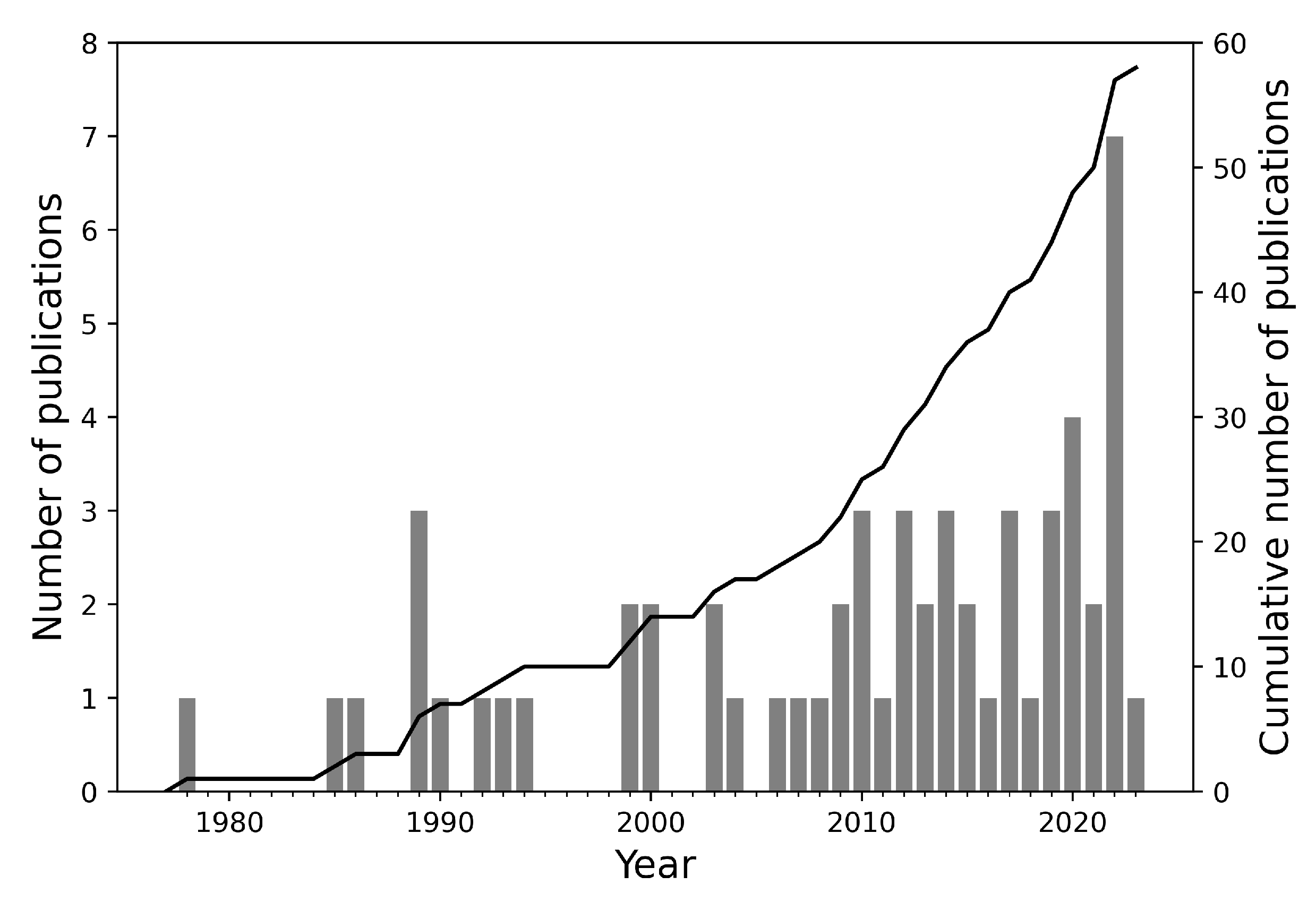
Figure 1. Number of papers from the open literature in which an estimation of the high-cycle fatigue strength was reported versus year of publication.
Metals 14 00085 g001
Figure 2. Geographic distribution of organisations affiliated with the first author of a paper in which an estimation of the high-cycle fatigue strength was reported.
Metals 14 00085 g002
Figure 3. Fatigue strength of specimens tempered at different temperatures for (a) rotating bending (the data at N = 10 9 are extrapolated) and (b) ultrasonic tensile loading. The legend indicates the tempering temperature and σ U [30]. Reproduced and adapted with permission from Zhao et al., Int. J. Fatigue; published by Elsevier, 2012.
Metals 14 00085 g003
Figure 4. (a) Relation between σ U and σ F σ U for 36CrNiMo. (b) Relation between σ U and σ F for 36CrNiMo [34]. Reproduced and adapted with permission from Pang et al., Mater. Sci. Eng. A; published by Elsevier, 2013.
Metals 14 00085 g004
Figure 5. Linear relations between σ F σ Y and σ Y σ U for steel alloys. The names in addition to the materials in the legend refer to the references from [39]. Reproduced and adapted with permission from Liu et al., J. Mater. Sci. Technol.; published by Elsevier, 2021.
Metals 14 00085 g005
Figure 6. Definition of σ C Y in a stable stress–strain hysteresis loop [37]. Reproduced and adapted with permission from Paul, Materalia; published by Elsevier, 2020.
Metals 14 00085 g006
Figure 7. Definition of the cyclic stress–strain curve as the locus of the tips of stable hysteresis loops [44]. Reproduced and adapted with permission from Hales et al., Mater. High. Temp.; published by Taylor & Francis, 2002.
Metals 14 00085 g007
Figure 8. Comparison of σ F calculated from estimations 58 and 59 for 250 MPa σ C Y 750 MPa .
Metals 14 00085 g008
Figure 9. Comparison of σ F calculated from estimations 60, 64, 65, and 69 for 100 kgf / mm 2 H V 400 kgf / mm 2 .
Metals 14 00085 g009
Figure 11. Relations between (a) σ F and H V , and (b) | e I I | and the ratio of the experimentally determined σ F to the estimation 1.6 · H V . Adapted from [57] (licensed under CC BY 4.0 (https://creativecommons.org/licenses/by/4.0/legalcode)).
Metals 14 00085 g011
Figure 12. Arbitrarily shaped surface crack in an infinite body loaded in uniform tension [60] (p. 20). Reproduced with permission from Murakami, Metal Fatigue: Effects of Small Defects and Nonmetallic Inclusions; published by Elsevier, 2019.
Metals 14 00085 g012
Figure 13. Periodic surface roughness pattern and equivalent notches [60] (p. 417). Reproduced with permission from Murakami, Metal Fatigue: Effects of Small Defects and Nonmetallic Inclusions; published by Elsevier, 2019.
Metals 14 00085 g013
Figure 14. Definition of a and b for estimation 100 for a random surface roughness pattern [65]. Reproduced with permission from Itoga et al., Int. J. Fatigue; published by Elsevier, 2003.
Metals 14 00085 g014
Figure 15. Definitions of σ k , σ G C F , B, b, N k , and N G C F used to describe the S–N curve (in a double logarithmic diagram) [73]. Reproduced and adapted with permission from Bandara et al., Comput. Mater. Sci.; published by Elsevier, 2015.
Metals 14 00085 g015
Table 3. Estimations for fatigue strength σ F based on ultimate tensile strength σ U and yield strength σ Y .
No.EstimationMaterial aGerman Equivalent (Material Number) b [21]RcTest Type c,dNumber of Cycles cNotesRef.
43 σ F = ( 18.486 + 0.503 · σ U
0.235 · 10 3 · σ U 2 ) · σ Y / σ U 0.75 0.4
DOMEX 350 YP/0R, UA 10 6 [41]
DOMEX 350 XP/
DOMEX 640 XPN/
DOMEX 490 XP/
44 σ F = σ Y 0.30 · 0.91 σ Y σ U Low-carbon steels −1RB/ [39]
45 σ F = σ Y 1.31 · 1.61 σ Y σ U Medium- and high-carbon steels −1RB/ [39]
46 σ F = σ Y 0.63 · 1.50 σ Y σ U SPCC
SPRC
DC01 (1.0330)
/
0UA 10 7 [39]
47 σ F = σ Y 1.08 · 1.50 σ Y σ U Si-Mn/−1RB 10 7 [39]
48 σ F = σ Y 0.76 · 1.33 σ Y σ U EN2440NiCrMo6 (1.6565)/// [39]
EN36/
49 σ F = σ Y 0.94 · 1.38 σ Y σ U EN56//// [39]
EN58X5CrNi18-10 (1.4301)
50 σ F = σ Y 1.28 · 1.28 σ Y σ U TWIP steel −1UA 10 7 [39]
51 σ F = σ Y 0.74 · 1.37 σ Y σ U TWIP steel 0.1UA 2 · 10 6 [39]
52 σ F = σ Y 1.12 · 1.49 σ Y σ U SAE1010C10E (1.1121)−1UA 4 · 10 6 [39]
53 σ F = 0.23 · σ Y + σ U Structural steels /// [19]
a /: no specific material was provided in the original source; b /: no equivalent material was found; c /: not provided in the original source; d R: resonance; RB: rotating bending; UA: uniaxial.
Table 4. Estimations for fatigue strength σ F based on cyclic yield strength σ C Y .
No.EstimationMaterial aGerman Equivalent (Material Number) b [21]RcTest Type c,dNumber of Cycles cNotesRef.
54 σ F = σ C Y DP600/−1UA 10 6 σ C Y determined by 0.01% offset in the loading branch of the hysteresis loop[37]
55 σ F = σ C Y ///B/ σ C Y determined by 0.1% offset in the cyclic stress–strain curve[23]
56 σ F = 0.554 · σ C Y SUS304X5CrNi18-10 (1.4301)−1UA/ σ C Y determined by 0.2% offset in the cyclic stress–strain curve[28]
57 σ F = 0.677 · σ C Y S25CC25 (1.0406)−1UA/ σ C Y determined by 0.2% offset in the cyclic stress–strain curve[28]
58 σ F = 0.865 · σ C Y S35CC35 (1.0501)−1UA/ σ C Y determined by 0.2% offset in the cyclic stress–strain curve[28]
S45CC45 (1.0503)
S55CC55 (1.0535)
SMn43836Mn6 (1.1127)
SMn44342Mn6 (1.1055)
SCr44041Cr4 (1.7035)
SCM43534CrMo4 (1.7220)
SCM44042CrMo4 (1.7225)
SNC63136NiCr10 (1.5736)
SNCM43940NiCrMo6 (1.6565)
SNCM44734CrNiMo6 (1.6582)
SUS430X6Cr17 (1.4016)
SUS403X6Cr13 (1.4000)
59 σ F = 1.13 · σ C Y 0.9 SAE 1141/−1UA 10 6 σ C Y determined by 0.2% offset in the cyclic stress–strain curve[43]
SAE 1038C35E (1.1181)
SAE 154136Mn6 (1.1127)
SAE 1050C50 (1.0540)
SAE 1090C92D (1.0618)
08/
20/
30/
40/
40CrNiMo40NiCrMo6 (1.6565)
60Si2Mn60Si7 (1.5027)
a /: no specific material was provided in the original source; b /: no equivalent material was found; c /: not provided in the original source; d B: bending; UA: uniaxial.
Table 7. Estimations for fatigue strength σ F based on Rockwell hardness H R .
No.EstimationMaterial aGerman Equivalent (Material Number) b [21]RcTest Type c,dNumber of Cycles cNotesRef.
79 σ F = ( 23.84 0.22 · H R C ) · H R C AISI 434036CrNiMo4 (1.6511)−1US 10 9 [19,34]
80 σ F = ( 24.73 0.19 · H R C ) · H R C SAE 434036CrNiMo4 (1.6511)−1RB/ [19]
81 σ F = ( 24.07 0.16 · H R C ) · H R C SAE 4063/−1RB/ [19]
82 σ F = ( 20.43 0.09 · H R C ) · H R C SAE 515046Cr2 (1.7006)−1RB/ [19]
83 σ F = ( 27.39 0.28 · H R C ) · H R C SAE 414042CrMo4 (1.7225)−1RB/ [19]
84 σ F = n · ( 2 · 10 7 ) b
n = n a · H R B p 3 + n b · H R B p 2 + n c · H R B p
Ferrous powder metal materials /UA 10 7 n a , n b , n c , and b: material dependent
H R B p : given by Equation (14)
[35]
a /: no specific material was provided in the original source; b /: no equivalent material was found; c /: not provided in the original source; d RB: rotating bending; UA: uniaxial; US: ultrasonic.
Table 13. Other estimations for the S–N curve.
No.EstimationMaterial aGerman Equivalent (Material Number) b [21]RcTest Type c,dNumber of Cycles cNotesRef.
130 σ F ( N ) = 1.62 · σ U · N 0.085 / −1/ 10 3 to 10 6 For σ U < 1400 MPa[81]
131 σ F ( N ) = σ U · N m

m = log 0.5 6 0.0502
/ −1RB/For σ U 1400 MPa[82]
132 log [ σ F ( N ) ] = log N A m

m = log N σ Y 10 6 log 0.9 · σ Y σ F ( 10 6 )

N σ Y = 400 · σ Y σ U 10

A = log 10 6 m · log [ σ F ( 10 6 ) ]
/ //1 to 10 9 Equations modified from those given in [83][83]
133 σ F ( N ) = A · log N + B
σ F ( 10 4 ) = 0.827 · σ U
A = 0.223 · σ F ( 10 4 ) 24.774
B = 1.8892 · σ F ( 10 4 ) 99.097
S10CC10E (1.1121) 1 RB 10 3 to 10 7 [48]
S15CC15E (1.1141)
S25CC25 (1.0406)
134 σ F ( N ) = A · log N + B S30CC30 (1.0528)−1RB 10 3 to 10 7 [48]
σ F ( 10 4 ) = 0.6556 · σ U S35CC35 (1.0501)
A = 0.4416 · σ F ( 10 4 ) 115.19 S45C (EQT)C45 (1.0503)
B = 2.7666 · σ F ( 10 4 ) 460.77 S50C (EQT)C50 (1.0540)
135 σ F ( N ) = A · log N + B
σ F ( 10 4 ) = 0.7083 · σ U
A = 0.2326 · σ F ( 10 4 ) 69.477
B = 1.9306 · σ F ( 10 4 ) 277.91
S45C (Q&T)C45 (1.0503)−1RB 10 3 to 10 7 [48]
S50C (Q&T)C50 (1.0540)
136 σ F ( N ) = 1 α t σ · 4 · ( 1 m ) · E · σ Y 2 · [ W ] ( 1 + ν ) · N 1 m 0.25

[ W ] = 0 ( ϵ t r ) f σ t r d ϵ t r 0.25 · σ Y + 3 · σ U 1 ψ n · ln 1 1 ψ n + 0.2 · σ U · 1 1 ψ n + 4 1 ψ · ln 1 ψ n 1 ψ
/ −1UA 10 5 to 10 10 m = 0.5 for body-centred cubic or face-centred cubic crystal lattice (steel and aluminium alloys)
m = 0.6 for hexagonal close-packed crystal lattice (titanium alloys)
α t σ = 1 for smooth specimens
[84]
137 σ F ( N ) = 1 α t σ · 4 · ( 1 m ) · E · σ Y 2 · [ W ] ( 1 + ν ) · ( 1 + R ) · N 1 m 0.25

[ W ] = 0 ( ϵ t r ) f σ t r d ϵ t r 0.25 · σ Y + 3 · σ U 1 ψ n · ln 1 1 ψ n + 0.2 · σ U · 1 1 ψ n + 4 1 ψ · ln 1 ψ n 1 ψ
/ >0UA 10 5 to 10 10 m = 0.5 for body-centred cubic or face-centred cubic crystal lattice (steel and aluminium alloys)
m = 0.6 for hexagonal close-packed crystal lattice (titanium alloys)
α t σ = 1 for smooth specimens
[84]
a /: no specific material was provided in the original source; b /: no equivalent material was found; c /: not provided in the original source; d RB: rotating bending; RT: reversed torsion; UA: uniaxial; US: ultrasonic.
Disclaimer/Publisher’s Note: The statements, opinions and data contained in all publications are solely those of the individual author(s) and contributor(s) and not of MDPI and/or the editor(s). MDPI and/or the editor(s) disclaim responsibility for any injury to people or property resulting from any ideas, methods, instructions or products referred to in the content.