Abstract
Incremental hole drilling is a commonly employed semi-destructive method for measuring internal residual stresses. It involves calculating internal residual stresses through the measurement of strains. The conversion of strain to stress is achieved through calibration coefficients, the accuracy of which directly influences the precision of residual stress measurements. These calibration coefficients are predominantly determined through finite element simulations, which must consider the sample’s characteristics and realistic experimental conditions. While there has been extensive research on the influence of sample thickness, the impact of thickness under different experimental conditions remains unexplored, and the underlying physical mechanisms driving thickness effects remain ambiguous. This paper addresses this gap by employing finite element simulations to investigate the impact of thickness on calibration coefficients under three commonly utilized experimental conditions. Moreover, this research endeavors to elucidate the physical mechanisms that contribute to variations in these coefficients through energy analysis.
1. Introduction
Residual stresses are an inevitable byproduct of materials processing and treatment [1]. Various mechanical manufacturing processes, such as casting, machining, welding, heat treatment, and assembly, all generate residual stresses in workpieces to varying degrees [2,3,4,5]. Residual stress is considered to be a crucial technical factor that must be considered when it comes to affecting the high-quality development of the manufacturing industry. Understanding the state of residual stresses serves as a fundamental foundation for assessing the engineering performance of materials and structural components [6]. Therefore, the accurate distribution and magnitude of residual stresses in materials hold both theoretical research and practical application value.
There are two main categories of residual stress measurement methods: non-destructive and destructive techniques. These include X-ray diffraction [7,8], neutron diffraction [9,10], layer removal methods [11,12], and the incremental hole-drilling method [13,14,15], among others. Each method has its applicability and limitations. The incremental hole-drilling method is often called a “semi-destructive method” due to the localized damage caused by drilling, which is limited to the hole-drilled area. The incremental hole-drilling method is a widely used technique for measuring residual stresses. It is applicable to most material structures, offering high reliability and accuracy. Standard testing procedures are available, and it is capable of measuring depth-dependent non-uniform residual stress fields without causing severe damage to the material. This method involves progressively drilling holes on the material’s surface. As the drilling removes stress material, it leads to redistribution of stress in the surrounding area, generating measurable local strains. Residual stresses at the original hole location are then evaluated based on the measured strains. The most common standard for the hole-drilling method is the American Society for Testing and Materials (ASTM) E837 standard measurement procedure [16,17]. This standard utilizes specially designed rosette strain gauges to measure strains and provides calibration factors under specific conditions. Surface strains can also be measured using optical techniques, such as moiré interferometry, Electronic Speckle Pattern Interferometry (ESPI), and Digital Image Correlation (DIC) [18,19,20,21,22,23,24], among others. Compared to traditional strain-gauge-based hole-drilling methods, optical measurement methods can eliminate the influence of strain gauge size and alignment difficulties on measurement results [25]. However, recalibration may be necessary depending on the measurement location and area size.
In the hole-drilling method, the evaluation of residual stresses by measured strains is performed utilizing calibration coefficients. The values of these calibration coefficients depend on factors such as hole diameter and hole depth. For different cases, the required calibration data can be determined by customized finite element calculations. The difference between the finite element model and the actual experimental situation can cause errors in calculating residual stresses. In previous studies, Blödorn [26] investigated the effect of the actual hole shape on the residual stress measurements, comparing the finite element model coefficients with chamfers and the finite element simulation coefficients without chamfers. Schajer [27] investigated the effect of structure thickness on calibration coefficients in the hole-drilling method and proposed a bivariate polynomial formula that represented the calibration data. This formula included 15 numerical coefficients, making it simpler to use and reducing calculation time. Schuster [28] considered the problem of plastic deformation near the hole due to the stress concentration effect of the hole in the case of hole drilling. Návrat [29] performed computational simulations of the hole-drilling experiments using the finite element method, analyzed the plastic effects of the hole-drilling method when measuring residual stresses, and performed plastic corrections by MATLAB. Peral [30] investigated the uncertainty associated with measuring non-uniform residual stresses using the hole-drilling method, taking into account factors such as material properties, hole depth, and diameter. Mamane [31] performed a numerical study to examine the impact of three experimental errors, namely incremental depth, strain gauge deflection angle, and hole eccentricity, on calibration coefficients in composite laminates. Additionally, a numerical correction method was developed to address the effects of these errors. Babaeeian [32] compared the hole-drilling and DIC methods in measuring residual stresses in composite plates, utilizing Mohr’s circle as an innovative approach. The study also analyzed the impact of strain measurement timing after drilling on residual stress measurements. Wu [33] proposed a more efficient correction method for the eccentricity error of the hole-drilling technique using a convolutional neural network. This new approach addresses the issue of eccentricity errors in hole drilling with greater ease.
With the trend towards lightweighting and thinwalling in various key industries such as aviation, aerospace, and automotive manufacturing, thin-walled structural components are being increasingly utilized. In order to meet the requirements of precision and dimensional stability for these thin-walled parts, it is necessary to understand and control the residual stresses present in thin-walled specimens. When it comes to thin-walled components, the thickness of the specimen has a significant impact on the calibration matrix when using the incremental hole-drilling method to measure residual stresses. Ignoring the influence of thickness can lead to severe deviations in residual stress measurements. On the other hand, for thick specimens, their inherent high rigidity ensures that the constraint method used during the drilling process does not affect the accuracy of residual stress measurements. In contrast, thin-walled specimens do not possess the same level of rigidity, and the influence of thickness during measurements varies under different constraint conditions. Historical research has primarily focused on the influence of specimen thickness on the calibration coefficients of the incremental hole-drilling method while neglecting the cumulative effects when combining experimental constraints with thickness. Furthermore, the physical mechanisms underlying the influence of thickness on the calibration coefficients of the incremental hole-drilling method remain unclear. In order to broaden the scope of measuring residual stresses in thin-walled components using the incremental hole-drilling method and to elucidate the physical mechanisms behind the distortion of the calibration coefficient matrix, further research is needed. This study considers three fundamental experimental constraint schemes during the hole-drilling measurement and evaluates the influence of specimen thickness on the calibration coefficients for each case. Moreover, leveraging the disparities in the forward and reverse energy releases during drilling, the study further unveils the physical mechanisms behind the calibration matrix distortion brought about by thickness variations.
2. Calculation of Calibration Coefficients for the Incremental Hole-Drilling Method Based on the Integral Method
There are multiple methodologies available for the calculation of residual stresses. A connection is established through computational algorithms between the measured released strains and the residual stresses. Among these, the integral method is recognized as one of the quintessential techniques for residual stress computation. It inherently accounts for the strain release prompted by the hole-drilling method. The measured strains are perceived as the collective outcome of all stresses acting throughout the depth. From these measured strains, the residual stresses are deduced. However, the relationship between the measured strain and the corresponding residual stress is expressed in the form of an inverse equation, making its solution more complex. The basis of the integration method is to transform a continuous problem into a set of discrete equations. In the case of incremental drilling, discretization is performed for each incremental step, and the relationship between stress and strain can be expressed as [16]
where represents the released strain at an angle with respect to the x-axis, E denotes the Young’s modulus, and is the Poisson’s ratio. , , and are matrices of the combined stresses. For a single layer, this can be expressed as
where , , and are the Cartesian stresses within the plane. P represents the isotropic biaxial stress, Q is the shear stress at , and T is the xy shear stress. is the calibration coefficient matrix associated with biaxial equal stress, while pertains to the shear stress calibration coefficient matrix. The number of entries within these matrices is contingent upon the drilling increments. For instance, when the drilling increment is five, the expanded forms of matrices and can be discerned from Equation (3).
Figure 1 illustrates the physical significance of each coefficient in matrix . From the figure, it can be observed that coefficient represents the strain caused by a unit stress within increment 2 of a hole 5 increments deep. The columns of the matrix represent the depth positions for equi-biaxial stresses, corresponding to the strain release at different hole depths. The rows of the matrix represent the strain release caused by different stress depths at a specified hole depth. The sum of the coefficients in each row represents the cumulative strain release of a uniform equi-biaxial stress field throughout the entire hole depth. Coefficient matrix has a similar physical significance to coefficient matrix , with the difference being that one utilizes an equi-biaxial stress field while the other employs a pure shear stress field. By examining the physical meaning of calibration coefficients and the matrix expansion, it can be observed that the calibration coefficient matrix is a lower triangular matrix. The rows of this matrix signify the influence of increasing hole depth, while the columns delineate the impact of stress depth.
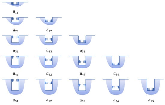
Figure 1.
Physical meaning of calibration coefficients.
3. Finite Element Model of Incremental Hole-Drilling Method Based on Three Constraint Conditions
Considering the constraints imposed by experimental conditions, the determination of calibration coefficients is indeed a formidable challenge. However, the introduction of finite element technology has rendered the computation of calibration coefficients not only feasible but also significantly more convenient. This research relies on finite element simulations to extract the calibration coefficients under diverse scenarios. The finite element models are established using ABAQUS 2020, encompassing models with dimensions of 40 mm in both length and width, as well as varying thicknesses. Ensure that the dimensions of the model are sufficient to simulate an infinitely large scenario. The fundamental parameters for these models are meticulously detailed in Table 1.

Table 1.
Finite element model parameter selection.
For the calculation of calibration coefficients and , two specific stress fields are utilized. The equi-biaxial stress solid model is employed for , while a pure shear stress solid model is used for . In this study, a known numerical stress field is applied to the material. The choice between using an equi-biaxial stress field or a pure shear stress field depends on whether to solve for the or coefficients. This study achieves the application of a known stress field by directly applying loads on the hole wall (Figure 1). The determination of calibration coefficients is independent of the magnitude of the applied load, but it is essential to ensure that the applied load does not exceed the material’s yield strength. This is because of the calibration coefficient determination by linear elastic models. Due to the use of linear elastic materials, the strain caused by a known stress is directly proportional to the magnitude of the stress. For computational convenience, this study uses a known stress of 1 MPa as an example for calculations. It necessitates the conversion from Cartesian coordinates to cylindrical coordinates. This transformation from Cartesian to cylindrical coordinates is a pivotal step in accurately replicating the experimental conditions for measuring residual stresses using the drilling method. The equations employed for executing this conversion are as follows:
From Equation (4), it is evident that the biaxial equal stress field can be transformed into a pressure of magnitude directly applied to the hole wall. The pure shear stress field can be expressed as shown in Equation (5). In this study, finite element simulation was performed using ABAQUS 2020. In Abaqus, both radial and shear loads can be applied by using a “surface traction” type of load, where the direction can be freely chosen, such as radial or tangential. This load also allows the use of analytical fields with trigonometric functions for the load distribution.
Figure 2a illustrates the dimensions of the strain gauge and the hole, with the strain gauge adopting the commonly used type-A strain gauge as defined in ASTM E837-20, i.e., mm, and the hole diameter mm. The area containing the strain gauge was delineated on the model’s surface, with the strain gauge’s length and width set to mm. To account for the influence of thickness on calibration coefficients in a non-uniform stress field, this study considers 20 incremental drilling steps, with each step having a drilling increment of 0.05 mm. The total hole depth is 1 mm. By extracting the strain values of all nodes within the strain gauge region, the average strain was calculated to simulate the surface strain measurement. Figure 2b illustrates the surface region of the three-dimensional finite element model established in ABAQUS. The model is discretized using linear hexahedral elements, precisely the C3D8R elements, which are known for their stable performance when the structure is subjected to bending loads. A unit size of 0.05 mm is utilized on the inner surface of the simulated hole drilling subjected to loading, with varying thickness models having approximately 150,000 to 250,000 grid elements. Model accuracy is validated by increasing mesh refinement, demonstrating that adopting a more precise grid does not impact the results. Additionally, a comparison between the calculated calibration coefficients of the thick specimen and the standard coefficients provided by ASTM E837-13a reveals a maximum error of approximately 5%, indicating that the model accuracy is sufficiently high.
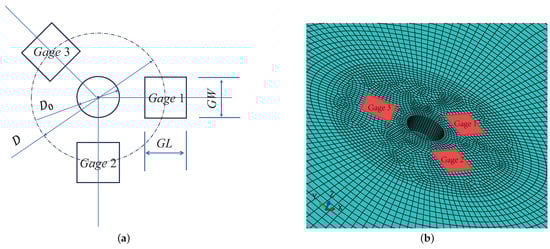
Figure 2.
Model surface schematic: (a) aperture and strain gauge size schematic; (b) finite element model surface view.
To accurately replicate the experimental conditions of the hole-drilling method, it is imperative to impose appropriate boundary conditions upon the model. Considering the more common experimental conditions in practice, three types of boundary conditions were considered. The first type of boundary condition corresponds to the scenario where the specimen is clamped on either two or all four sides during measurement, leaving the bottom completely free. In this case, the finite element model is simulated with all four sides fixed and the bottom degrees of freedom wholly released. It can be seen from Figure 3a. The second type of boundary condition corresponds to a scenario in which the edges of the sample are fixed during measurement while the bottom of the sample is supported. It can be seen from Figure 3b. In this case, this study added a fixed support structure at the bottom of the model, treating it as a rigid body without considering its deformation while applying fixed constraints to all four sides. As shown in Figure 4, a supporting rigid body was added to the bottom of the model. The third type of boundary condition corresponds to the scenario where measures to resist bending are applied during measurement. Thin-walled specimens, due to their lower stiffness, are sometimes subjected to measures to reduce deformation during testing. It can be seen from Figure 3c. In this case, fix all four edges of the finite element model, with the bottom’s Z-direction degrees of freedom constrained.
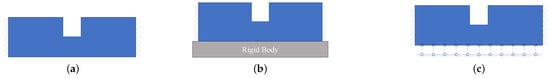
Figure 3.
Finite element model boundary condition schematic: (a) bottom free constraint situation; (b) bottom support constraint situation; (c) bottom Z-direction degrees of freedom constraints situation.
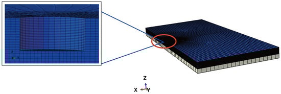
Figure 4.
The support boundary condition, and a detailed view of the incremental step direction meshing.
4. Results and Discussion
4.1. Analysis of the Bottom Free Constraint Situation
In the process of measurement using the hole-drilling method, the measurement location and conditions during measurement are predominantly determined by the specific measurement requirements. The measurement of an object’s shape itself can affect the constraints applied during the measurement process, similar to thin-walled structures such as composite pipes or turbine casings. In practical measurements, due to the inherent shape limitations, the bottom of the measurement location often lacks support constraints and remains completely free. Additionally, for most researchers, measuring residual stresses with the bottom being free is preferred because it eliminates the need for additional fixtures and offers greater convenience in measurement. Therefore, in most cases, measurements are conducted with the specimen in a condition of bottom freedom, corresponding to the finite element calibration coefficients simulated in ASTM E837. In this scenario, the model is fixed around its periphery while allowing complete freedom of movement at the bottom. Based on the boundary condition of bottom freedom (Figure 3a), this study conducted finite element simulations on specimens of different thicknesses. During the finite element simulations, known equi-biaxial stress fields and pure shear stress fields were applied, and the strains in three strain gauge regions were calculated. By combining the integration method described in Section 2, calibration coefficients and , as shown in Figure 5, can be calculated.
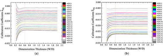
Figure 5.
Thickness effect on calibration coefficients with bottom freedom: (a) calibration coefficients ; (b) calibration coefficients .
A finite element model with a hole radius of 1mm was employed to assess the influence of thickness on calibration coefficients under the condition of bottom freedom. Figure 5 illustrates the variation in calibration coefficients for the 20th row of the matrix and matrix. As dimensionless thickness is less than 0.6, a noticeable change in calibration coefficient is observed. This phenomenon underscores the rationale behind ASTM’s stipulation of a minimum thickness of 0.6 D for thick specimens. Moreover, calibration coefficients at different stress depths exhibit two distinct trends with changes in thickness depending on whether load is applied near the bottom or the top of the hole. For a twenty-step increment, the approximate transition point in trends can be around the tenth or eleventh increment. As thickness decreases, there is a notable increase in the numerical values of calibration coefficients when load is applied at the top of the hole, signifying continuous growth in compressive strain within the strain field region. Conversely, when load is applied at the bottom of the hole, calibration coefficients transition from negative to positive values, indicating a transformation within the surface strain field region from compressive to tensile strain. Coefficient exhibits trends similar to coefficient but with smoother changes in its coefficients. Furthermore, even when load is applied at the bottom of the hole, positive coefficients do not occur. While two distinct trends can be clearly observed in the case of coefficient , only minor variations are noticeable in the case of coefficient . The differences in trends between coefficients and arise because one is calculated using a equi-biaxial stress model. At the same time, the other employs a pure shear stress model during the calculation. J.M. Alegre [34] investigated the impact of thickness on calibration coefficient under type-B rosette conditions. Upon comparison, it is evident that the trends in coefficient are similar, but differences are observed in coefficient . This disparity can be attributed to the broader gauge width of the type-A rosette.
Under bottom unconstrained conditions, Marco Beghini [35] and A. Magnier [36] demonstrated through experiments that customized calibration coefficients are needed for thin-walled specimens. In Marco Beghini’s study, pre-stress was applied in tension experiments, and hole drilling tests were conducted in a known uniform stress field. Residual stresses were then calculated using custom thickness calibration coefficients. The calibration coefficient changes in his work align with the trend provided by finite element simulations in this study. A. Magnier’s work involved bending experiments on three different thicknesses of thin plates, applying a non-uniform stress field. After obtaining strain release through drilling tests, stresses were calculated using custom calibration coefficients for the three thicknesses. This experiment better illustrates the impact of thickness on calibration coefficients in the case of a non-uniform stress field. The article provides calibration coefficient tables for the three thicknesses, and, by comparing the last row of the calibration coefficient matrices for the three thicknesses, it can be observed that the coefficients exhibit two different trends with stress depth, consistent with the trends in the finite element results in this study. By comparing the finite element simulations with the experimental results, the correctness of the finite element simulations is validated.
4.2. Analysis of the Bottom Support Constraint Situation
During measurements, due to the relatively low bending stiffness of the test specimen itself and the downward bending induced by hole-drilling experiments, some researchers may choose to add a support structure at the bottom of the sample where drilling occurs to prevent bending. This support is primarily aimed at addressing bending caused by external factors. From the observed variation in the calibration coefficient under unconstrained conditions at the bottom, it can be inferred that, when a load is applied at the bottom of the hole, the surface exhibits tensile stress. The release of internal stress leads to a slight downward bending of the specimen. This study does not consider bending caused by external factors but focuses on the internal stress release. It considers adding a support structure at the bottom of the specimen to analyze the influence of thickness on calibration coefficients in the presence of support. Based on the boundary condition of bottom support (Figure 3b), this study conducted finite element simulations on specimens of different thicknesses. The obtained calibration coefficients and are shown in Figure 6.
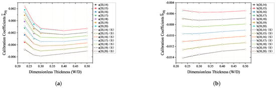
Figure 6.
Thickness effect on calibration coefficients when there is support at the bottom: (a) calibration coefficients ; (b) calibration coefficients .
By observing the calibration coefficients under the bottom support model, it is evident that, when the specimen thickness is relatively large or when load is applied far from the bottom of the hole, the calibration coefficients are generally consistent with those obtained under bottom unconstrained conditions. However, when load is applied near the bottom of the hole, and the specimen thickness is relatively thin, the support structure does have a specific influence on the calibration coefficients. Figure 6 includes a comparison between the calibration coefficients under bottom support constraints and those under bottom unconstrained conditions. The dashed line represents the calibration coefficients under bottom unconstrained conditions, while the solid line represents the calibration coefficients under bottom support constraints. From Figure 6, it is evident that coefficient remains the same as coefficient under bottom unconstrained conditions, regardless of stress depth or thickness. When the dimensionless thickness is less than 0.4, there are certain discrepancies in coefficient compared to coefficient under bottom unconstrained conditions. As the thickness decreases, more incremental steps exhibit errors. At a dimensionless thickness of 0.23, when load is applied near the hole bottom, the maximum error between the calibration coefficients under bottom support constraints and those under bottom unconstrained conditions can reach up to 60%. The cause of this phenomenon is attributed to the effect of bottom support. When the non-dimensional thickness is within the range of 0.2 to 0.4, loading near the bottom of the hole induces a downward bending trend in the specimen. Note that there is no occurrence of downward bending when solving for coefficient using a pure shear force model. When the specimen undergoes downward bending, the support at the bottom provides a supporting force, thereby affecting the calibration coefficients. Figure 7 illustrates the deformation trend of the model when support is present and load is applied at the hole bottom. The bottom support force mainly concentrates beneath the hole wall, leading to changes in the calibration coefficients.
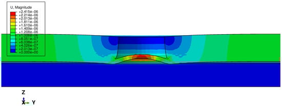
Figure 7.
The deformation trends of the model under the presence of support constraints and load applied at the bottom of the hole; the trend is amplified for greater visibility.
4.3. Analysis of Bottom Z-Direction Degrees of Freedom Constraints Situation
The measurement of thin-walled components has long been a focal point for researchers, with particular attention directed toward addressing bending effects. In addition to incorporating support structures at the base of thin-walled components, some researchers employ more robust methods to counteract the bending phenomenon. For instance, affixing the lower portion of the test specimen to the support structure using super glue serves a dual purpose by not only preventing downward bending but also immobilizing the base, thus averting any upward bending [37]. Additionally, specific fixtures can be employed to effectively restrict both the upward and downward bending of the test specimen. Such constraints primarily act upon the bottom of the specimen and do not involve the specimen’s surface to prevent any impact on the specimen’s surface, thereby minimizing the introduction of extraneous stress. When calibrating the coefficients for such constraints, adjustments can be made by configuring the degrees of freedom at the bottom of the model. Given that there is minimal distinction between fully fixing the bottom and only constraining the Z-direction degrees of freedom at the bottom in terms of their impact on the surface, in order to accommodate a broader range of fixture scenarios, this study examines the influence of thickness on calibration coefficients under the constraint of limiting the Z-direction degrees of freedom at the model’s bottom. Furthermore, the distribution ratio of energy also elucidates the physical mechanisms through which thickness exerts its influence under the constraint of bottom Z-direction degrees of freedom.
In previous research, the author in [38] studied the variation in calibration coefficients with thickness under limited Z-direction freedom at the bottom in a uniform stress field. This was completed by applying a uniform stress field to a thin aluminum plate in tensile experiments and using specific fixtures that significantly reduce bending during drilling, effectively equivalent to restricting the Z-direction freedom at the bottom of the specimen. Based on this experimental setup, calibration coefficients for thin specimens in a uniform stress field were calculated using a finite element model with constrained Z-direction freedom at the bottom. The residual stresses calculated using these coefficients were closer to the pre-stress than those calculated using ASTM standard calibration coefficients. It can be demonstrated that, during measurement, if there is a limitation on the Z-direction freedom at the bottom of the specimen, employing a model with Z-direction constraints at the bottom will result in more accurate residual stress calculations. In this study, the finite element model with Z-direction freedom constraints at the bottom is utilized to focus on the variation in calibration coefficients with thickness under non-uniform stress fields, thereby providing greater assistance in expanding the application range of the drilling method.
Figure 8 corresponds to a hole depth of 1 mm, illustrating the influence of thickness on the calibration coefficients of the 20th row in matrix and the 20th row in matrix when subjected to Z-direction degrees of freedom constraints at the bottom. Based on the graph, it can be observed that, when the dimensionless thickness exceeds 0.7, the thickness has minimal impact on the calibration coefficient. However, when the thickness is below 0.7, significant differences in the calibration coefficient can be observed with varying thicknesses. Furthermore, both coefficient and coefficient exhibit two distinct trends in their variations. Regarding coefficient , regardless of the incremental steps, two distinct trends can be observed. The approximate boundary between these two trends can occur at a dimensionless thickness of 0.3 in the specimens. When the dimensionless thickness ranges from 0.3 to 0.7, as the thickness decreases, the absolute value of the calibration coefficient also decreases continuously. However, when the dimensionless thickness ranges from 0.2 to 0.3, as the thickness decreases, the absolute value of the calibration coefficient starts to increase. Regarding coefficient , two distinct trends are observed when the load is applied within a distance of 0.35 mm from the bottom of the hole. In this case, the variation trend is similar to that of coefficient . However, for remaining coefficients , the trend shows a continuous decrease in absolute value as the thickness decreases. It is worth noting that, in the case of bottom Z-constraint, the calibration coefficients are all negative, and the variation trends are essentially opposite to those of the calibration coefficients under bottom free conditions. This phenomenon can be attributed to the influence of bottom constraint on the release of surface strains.
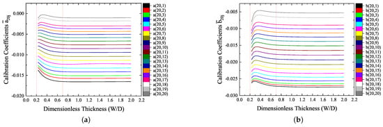
Figure 8.
Thickness effect on calibration coefficients in preventing bending conditions: (a) calibration coefficients ; (b) calibration coefficients .
To gain a more comprehensive understanding of the physical mechanism behind the impact of thickness when the Z-direction freedom at the bottom is constrained, this study will analyze from the perspectives of the overall model, surface, and bottom strain energy, with a focus on the distribution of energy. Using ABAQUS 2020, different thicknesses and stress depths were considered in a biaxial stress model. The energy (ALLSE) at three locations was extracted: the total strain energy of the entire plate, the strain energy within the surface strain gauge region of the plate (as shown in Figure 9, including the total strain energy of strain gauges 1–3), and the strain energy within the strain gauge region of the bottom surface of the plate (as shown in Figure 9, including the total strain energy of strain gauges 4–6).
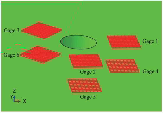
Figure 9.
Schematic diagram of strain energy extraction locations.
Figure 10a–c depict the strain energy at the overall, surface, and bottom surface, respectively, when employing the equal biaxial stress model at different stress depths. From Figure 10a, it can be observed that the location of load application significantly affects the energy of the model. When the load is applied closer to the top of the hole, the overall strain energy is more significant. Conversely, when the load is applied at the bottom of the hole, the overall strain energy of the model is minimized. The bottom constraint primarily causes this phenomenon. When the dimensionless thickness exceeds 0.4, the overall strain energy remains relatively constant. However, when the dimensionless thickness is in the range of 0.2 to 0.4, as the thickness decreases, the overall strain energy shows an increasing trend. Moreover, when the load is applied near the bottom of the hole, the variation in strain energy becomes more pronounced. Despite the Z-direction constraint applied to the bottom of the model, it is evident that, as the thickness decreases, the deformation of the model continues to increase. As shown in Figure 10b, the variation in strain energy at the surface strain gauges differs from that of the overall strain energy. The change in surface strain energy exhibits a similar trend to that of coefficient . Figure 10c demonstrates the variation in strain energy at the bottom corresponding to the region of surface strain gauges with respect to thickness. It is evident that the strain energy at the bottom consistently increases as the thickness decreases.
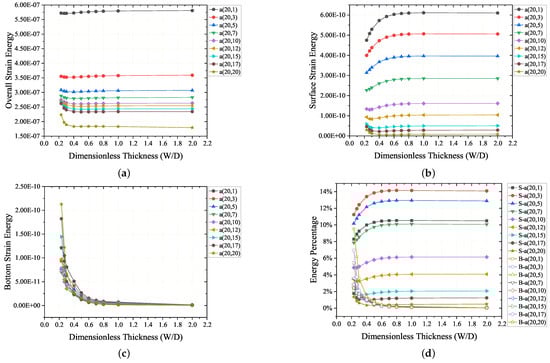
Figure 10.
Thickness effect on model energy in preventing bending conditions: (a) overall strain energy; (b) surface strain energy; (c) bottom surface strain energy; (d) energy percentage.
Based on the energy variation in the model considering the Z-direction constraint at the bottom, it can be observed that, for a given hole depth and unit stress layer depth, when the dimensionless thickness is between 0.3 and 0.7, the reduction in thickness leads to a decrease in the strain energy at the surface of the biaxial equal stress model. In contrast, the strain energy at the bottom surface continues to increase. Regarding this phenomenon, it can be inferred that, as the thickness decreases, the stress-induced strain energy is dispersed more towards the bottom surface, resulting in a decrease in the surface strain energy. However, due to factors such as the location of load application, the strain energy levels of the surface and bottom regions inherently exhibit significant differences, making direct comparison challenging. Therefore, in this study, the proportion of energy from the surface and bottom regions to the total energy will be calculated and compared. This approach will provide more favorable support for interpretation. Based on Figure 10d, it is evident that, except for the case where load is applied at the bottom of the hole and the dimensionless thickness is less than 0.3, there is a consistent trend of decreasing proportion in surface strain energy and increasing proportion in bottom strain energy as thickness decreases. In the scenario where load is applied at the bottom, it can be inferred that, due to the excessively small thickness, the overall, surface, and bottom strain energy all increase, which sets it apart from the other incremental steps.
In summary, although the Z-direction constraint applied to the bottom effectively restrains the bending deformation of the specimen, it does not prevent the influence of thickness on the calibration coefficient. The reason for the decrease in the absolute value of the calibration coefficient can be explained by the energy distribution. As the thickness decreases, more energy is dispersed towards the bottom of the specimen rather than the surface, resulting in a decrease in surface strain and a subsequent change in the calibration coefficient.
5. Conclusions
This study investigates the influence of thickness on the calibration coefficient in the incremental hole-drilling method under three main measurement constraint conditions. These constraint conditions can be categorized as a complete release of constraints at the bottom of the specimen, presence of support constraints at the bottom of the specimen, and Z-direction constraint at the bottom of the specimen. The accuracy of the calibration coefficient directly affects the reliability of the incremental drilling method measurement. By analyzing the impact of thickness on the calibration coefficient under different constraint conditions and studying the physical mechanisms of thickness effects, this research aims to provide further insights into regulating the thickness effect.
When the non-dimensional thickness is above 0.4, the calibration coefficients obtained under two conditions, namely bottom unconstrained and bottom with support constraints, exhibit a high level of consistency. However, when the non-dimensional thickness is within the range of 0.2 to 0.4 and a load is applied near the bottom of the hole with support constraints, there is a noticeable difference in the calibration coefficient compared to when there are no constraints at the bottom. This difference can be attributed to the fact that, when the non-dimensional thickness is greater than 0.4, even with loading near the bottom of the hole, it does not induce a downward bending trend in the specimen, thereby ensuring that bottom support does not affect the calibration coefficients. In both cases of unconstrained bottom and the presence of support constraints, the influence of thickness occurs within the dimensionless thickness range of 0.2 to 0.6. Calibration coefficients exhibit two entirely distinct trends. The specific trend is dependent on the location of the applied load. In this case, the thickness effect is primarily due to the lack of constraint at the bottom of the specimen, where a decrease in thickness results in lower stiffness at the bottom, leading to bending deformation. The Z-direction constraint at the bottom exhibits significant differences in trend compared to the other two constraint conditions. Its influence occurs within the range of dimensionless thickness from 0.2 to 0.7, where there are also two distinct trends. The boundary between the two trends can be considered at a dimensionless thickness of 0.3. Under this constraint condition, the thickness effect is primarily due to the reduction in specimen thickness, which results in a more significant transfer of energy from the surface to the bottom. Consequently, the surface strain decreases, leading to a change in the calibration coefficient. When measuring residual stresses in thin-walled components using the incremental drilling method, employing specific calibration coefficients for different constraint conditions is a practical approach to enhance the accuracy of residual stress measurements.
Author Contributions
Conceptualization, K.Z., Y.C. and S.X.; methodology, Y.C., K.Z. and S.X.; software, Y.C.; writing—original draft, Y.C. and S.X.; writing—review and editing, K.Z. and Y.C. All authors have read and agreed to the published version of the manuscript.
Funding
This work was supported by the National Natural Science Foundation of China (Grant number 11802316) and the Changzhou Longcheng talent plan (Grant number CQ20210045), as well as the National Engineering and Research Center for Commercial Aircraft Manufacturing under Grant No. COMAC-SFGS-2022-1874.
Data Availability Statement
The data presented in this study are available in article.
Acknowledgments
The authors of this study extend gratitude to the following five researchers for their valuable assistance: Pei Zheng, Zhenya Zhang, Jia Huang, Wencheng Liu, and Jun Yao.
Conflicts of Interest
The authors declare no conflicts of interest.
References
- Tabatabaeian, A.; Ghasemi, A.R.; Shokrieh, M.M.; Marzbanrad, B.; Baraheni, M.; Fotouhi, M. Residual Stress in Engineering Materials: A Review. Adv. Eng. Mater. 2021, 24, 2100786. [Google Scholar] [CrossRef]
- Fajoui, J.; Kchaou, M.; Sellami, A.; Branchu, S.; Elleuch, R.; Jacquemin, F. Impact of residual stresses on mechanical behaviour of hot work steels. Eng. Fail. Anal. 2018, 94, 33–40. [Google Scholar] [CrossRef]
- Chen, S.; Gao, H.; Zhang, Y.; Wu, Q.; Gao, Z.; Zhou, X. Review on residual stresses in metal additive manufacturing: Formation mechanisms, parameter dependencies, prediction and control approaches. J. Mater. Res. Technol. 2022, 17, 2950–2974. [Google Scholar] [CrossRef]
- Yi, R.; Chen, C.; Shi, C.; Li, Y.; Li, H.; Ma, Y. Research advances in residual thermal stress of ceramic/metal brazes. Ceram. Int. 2021, 47, 20807–20820. [Google Scholar] [CrossRef]
- Diaz, A.; Cuesta, I.I.; Alegre, J.M.; de Jesus, A.M.P.; Manso, J.M. Residual stresses in cold-formed steel members: Review of measurement methods and numerical modelling. Thin-Walled Struct. 2021, 159, 107335. [Google Scholar] [CrossRef]
- Guo, J.; Fu, H.; Pan, B.; Kang, R. Recent progress of residual stress measurement methods: A review. Chin. J. Aeronaut. 2021, 34, 54–78. [Google Scholar] [CrossRef]
- Yazdanmehr, A.; Jahed, H. On the Surface Residual Stress Measurement in Magnesium Alloys Using X-Ray Diffraction. Materials 2020, 13, 5190. [Google Scholar] [CrossRef]
- Taisei, D.; Masayuki, N.; Junichi, O. Residual Stress Measurement of Industrial Polymers by X-ray Diffraction. Adv. Mat. Res 2015, 1110, 100–103. [Google Scholar] [CrossRef]
- Sun, G.; Chen, B. The technology and application of residual stress analysis by neutron diffraction. Nucl. Tech. 2007, 30, 286–289. [Google Scholar]
- Li, J.; Wang, H.; Sun, G.; Chen, B.; Chen, Y.; Pang, B.; Zhang, Y.; Wang, Y.; Zhang, C.; Gong, J.; et al. Neutron diffractometer RSND for residual stress analysis at CAEP. Nucl. Instrum. Meth. A. 2015, 783, 76–79. [Google Scholar] [CrossRef]
- Carpenter, H.W.; Reid, R.G.; Paskaramoorthy, R. Sensitivity Analysis of the Crack Compliance and Layer Removal Methods for Residual Stress Measurement in GFRP Pipes. J. Appl. Mech. Trans. ASME 2016, 138, 031001. [Google Scholar] [CrossRef]
- Liu, L.; Sun, J.; Chen, W.; Chen, Q. Study on Distribution of Initial Residual Stress in 7075T651 Aluminium Alloy Plate. China Mech. Eng. 2016, 27, 537–543. [Google Scholar]
- Kim, C.H. Investigation on the Hole-producing Techniques of Residual-stress Measurement by Incremental Hole-drilling Method in Injection Molded Part. Fibers Polym. 2018, 19, 1776–1780. [Google Scholar] [CrossRef]
- Jiang, H.; Zhou, L.; Lu, J. A Computational Method of Residual Stress Calculation for Incremental Hole-Drilling Method Utilized Composite Materials. Mater. Sci. Forum. 2015, 813, 94–101. [Google Scholar] [CrossRef]
- Schajer, G.S.; Rickert, T.J. Incremental Computation Technique for Residual Stress Calculations Using the Integral Method. Exp. Mech. 2011, 51, 1217–1222. [Google Scholar] [CrossRef]
- ASTM E837-13a; Standard Test Method for Determining Residual Stresses by the Hole Drilling Strain-Gage Method. ASTM International: West Conshohocken, PA, USA, 2013.
- ASTM E837-20; Standard Test Method for Determining Residual Stresses by the Hole-Drilling Strain-Gage Method. ASTM International: West Conshohocken, PA, USA, 2020.
- Zhang, K.; Yuan, M.; Chen, J. General Calibration Formulas for Incremental Hole Drilling Optical Measurement. Exp. Tech. 2017, 41, 1–8. [Google Scholar] [CrossRef]
- Wu, Z.; Lu, J.; Han, B. Study of residual stress distribution by a combined method of moire interferometry and incremental hole drilling, part II: Implementation. J. Appl. Mech.-Trans. ASME 1998, 65, 844–850. [Google Scholar] [CrossRef]
- Schajer, G.S.; Steinzig, M. Dual-Axis Hole-Drilling ESPI Residual Stress Measurements. J. Appl. Mech.-Trans. ASME 2010, 132, 011007. [Google Scholar] [CrossRef]
- Pisarev, V.; Odintsev, I.; Eleonsky, S.; Apalkov, A. Residual stress determination by optical interferometric measurements of hole diameter increments. Opt. Laser Eng. 2018, 110, 437–456. [Google Scholar] [CrossRef]
- Baldi, A. On the Implementation of the Integral Method for Residual Stress Measurement by Integrated Digital Image Correlation. Exp. Mech. 2019, 59, 1007–1020. [Google Scholar] [CrossRef]
- Xu, Y.; Bao, R. Residual stress determination in friction stir butt welded joints using a digital image correlation-aided slitting technique. Chin. J. Aeronaut. 2017, 30, 1258–1269. [Google Scholar] [CrossRef]
- Brynk, T. Application of 3D DIC Displacement Field Measurement in Residual Stress Calculations. Adv. Mater. Sci. 2017, 17, 46–53. [Google Scholar] [CrossRef][Green Version]
- Nelson, D.V. Residual stress determination using full-field optical methods. J. Phys. Photonics 2021, 3, 044003. [Google Scholar] [CrossRef]
- Blödorn, R.; Bonomo, L.; Viotti, M.; Schroeter, R.; Albertazzi, A., Jr. Calibration Coefficients Determination Through Fem Simulations for the Hole-Drilling Method Considering the Real Hole Geometry. Exp. Tech. 2016, 41, 37–44. [Google Scholar] [CrossRef]
- Schajer, G. Compact Calibration Data for Hole-Drilling Residual Stress Measurements in Finite-Thickness Specimens. Exp. Mech. 2020, 60, 665–678. [Google Scholar] [CrossRef]
- Schuster, S.; Steinzig, M.; Gibmeier, J. Incremental Hole Drilling for Residual Stress Analysis of Thin Walled Components with Regard to Plasticity Effects. Exp. Mech. 2017, 57, 1457–1467. [Google Scholar] [CrossRef]
- Návrat, T.; Halabuk, D.; Vosynek, P. Efficiency of Plasticity Correction in the Hole-Drilling Residual Stress Measurement. Materials 2020, 13, 3396. [Google Scholar] [CrossRef]
- Peral, D.; de Vicente, J.; Porro, J.; Ocaña, J. Uncertainty analysis for non-uniform residual stresses determined by the hole drilling strain gauge method. Measurement 2017, 97, 51–63. [Google Scholar] [CrossRef]
- Mamane, A.I.; Giljean, S.; Pac, M.J.; L’Hostis, G. Optimization of the measurement of residual stresses by the incremental hole drilling method. Part I: Numerical correction of experimental errors by a configurable numerical–experimental coupling. Compos. Struct. 2022, 294, 115703. [Google Scholar] [CrossRef]
- Babaeeian, M.; Mohammadimehr, M. Investigation of the time elapsed effect on residual stress measurement in a composite plate by DIC method. Opt. Laser Eng. 2020, 128, 106002. [Google Scholar] [CrossRef]
- Wu, J.; Qiang, B.; Liao, X.; Huang, Y.; Changrong, Y.; Li, Y. Hole-drilling method eccentricity error correction using a convolutional neural network. J. Strain Anal. Eng. Des. 2022, 58, 030932472210800. [Google Scholar] [CrossRef]
- Alegre, J.M.; Díaz, A.; Cuesta, I.I.; Manso, J.M. Analysis of the Influence of the Thickness and the Hole Radius on the Calibration Coefficients in the Hole-Drilling Method for the Determination of Non-uniform Residual Stresses. Exp. Mech. 2019, 59, 79–94. [Google Scholar] [CrossRef]
- Beghini, M.; Bertini, L.; Giri, A.; Santus, C.; Valentini, E. Measuring residual stress in finite thickness plates using the hole-drilling method. J. Strain Anal. Eng. Des. 2019, 54, 65–75. [Google Scholar] [CrossRef]
- Magnier, A.; Zinn, W.; Niendorf, T.; Scholtes, B. Residual Stress Analysis on Thin Metal Sheets Using the Incremental Hole Drilling Method—Fundamentals and Validation. Exp. Tech. 2019, 43, 65–79. [Google Scholar] [CrossRef]
- Hosseini, S.; Akbari, S.; Shokrieh, M. Residual stress measurement through the thickness of ball grid array microelectronics packages using incremental hole drilling. Microelectron. Reliab. 2019, 102, 113473. [Google Scholar] [CrossRef]
- Zhang, K.; Zhou, Y.; Zhao, S.; Chen, J. Numerical and experimental investigation of thickness effect on residual stress measurement. Mat. Sci. Technol. 2016, 32, 1495–1504. [Google Scholar] [CrossRef]
Disclaimer/Publisher’s Note: The statements, opinions and data contained in all publications are solely those of the individual author(s) and contributor(s) and not of MDPI and/or the editor(s). MDPI and/or the editor(s) disclaim responsibility for any injury to people or property resulting from any ideas, methods, instructions or products referred to in the content. |
© 2024 by the authors. Licensee MDPI, Basel, Switzerland. This article is an open access article distributed under the terms and conditions of the Creative Commons Attribution (CC BY) license (https://creativecommons.org/licenses/by/4.0/).