Abstract
Theoretical models based on solutions of the conduction heat transfer equation have been widely proposed to calculate the thermal fields generated during laser welding, revealing simplification benefits and limitations in the accuracy of the results. In previous papers, the authors have introduced a parameterized analytical model based on the configuration of a virtual system of multiple mobile heat sources that simulates the effects of an actual keyhole welding mode by setting the system parameters so as to fit the calculated contours of the fusion zone in the weld cross-section of the experimental one. Even though a basic validation was already carried out by experimental detection, in order to further strengthen the model validity, this article deals with an extensive comparison between the results obtained by a multi-physics numerical simulation, performed by a commercial CFD software, and a theoretical one. The two different approaches were applied to the laser beam welding of butt-positioned AISI 304L steel plates. The investigation was focused on the effects of the keyhole on the main morphological features of the melt pool and fusion zone, and on the thermal fields obtained by the two models. The intrinsic differences between the two approaches, and how they are reflected in the corresponding results, were discussed. Satisfactory results were obtained by comparing the thermal fields, with a substantial convergence of the results, so as to validate the analytical model, assess the accuracy of its results, and define its application limits.
1. Introduction
In the field of joining metallic materials, laser beam welding continues to play a key role due to the concentrated high power density heat input, which allows for a high accuracy in welding thick workpieces in a single pass, producing narrow heat affected zones (HAZs) and limited thermal distortions. For this reason, investigations on the various aspects of laser welding, from the laser–material interaction, to welding phenomena, defect formation mechanisms, and process monitoring and control, always remain subjects of study [1], and new technological solutions continue to arise to improve the efficiency of the process, such as spatial beam shaping, based on multiple focusing which enables one to customize the energy distribution [2], and multiple micro-jet cooling with shielding gas. The latter is very promising in terms of governing the final microstructure of the weld metal deposit, such as in the case of low alloy steel, with significant beneficial effects on the impact toughness of welds [3]. The implications in terms of the environmental efficiency of the process are also considered worthy of attention [4].
The integrity of the welded parts and every technical requirement that are to be ensured, such as primarily the weld quality and efficiency, depend on laser beam characteristics, material properties, process parameters, and the thermal field that their combination generates. Consequently, laser beam welding process modelling, including the main characteristics of the weld joint (geometrical, metallurgical, and mechanical), is a subject of great interest [5]. In order to predict the effects of the parameter settings on the final joint and evaluate its mechanical and metallurgical features as well as the occurrence of distortion and residual stress, both analytical and numerical models based on the solutions of the conduction heat transfer equation have been widely proposed to simulate the thermal fields generated during laser welding [6]. A complete formalization of the theoretical basis for this approach, with a detailed overview on the formulation and solution of heat conduction problems in fusion welding has also been provided [7].
Numerical models can cover a wide spectrum of physical and thermal processes occurring during welding. A detailed review on the main aspects of welding simulations by finite element methods (FEMs) has been presented, highlighting the key role of increasing the complexity of the models to improve the reliability and effectiveness in describing the engineering applications [8]. The importance of material modelling [9] and computational efficiency [10] have also been clearly outlined. More recently, an overview on the approaches to finite element modelling used to simulate fusion weld processes has been provided, analyzing the level of accuracy when comparing the results of simulations with experiments [11].
Particularly, high computational capacities and simulation times are required for modelling effectively complex processes such as fusion welding, which involve the interaction between physical and metallurgical phenomena, even if a number of simplifications are commonly assumed in finite element models [12]. Furthermore, the simulations have to be validated, generally by using the results of experimental measurements, to be considered specific to the particular welding conditions that are adopted.
The basic analytical solutions of the heat conduction equation have also been widely used for modelling the thermal field in welding processes. Their use allows for a less complex approach from a computational point of view, and has given satisfactory results in comparison with experimental data, although involving a considerable simplification of the phenomenon to be modelled. Rosenthal’s seminal contribution with its solutions for the case of moving point and line heat sources in infinite and semi-infinite media [13], and a later complete framework of solutions of the heat conduction in solids [14], constitute the basis on which a large part of the analytical models for laser welding processes have been developed, allowing one to simulate the temperature profiles generated by moving sources of various types [6], and to continue to constitute the basic reference for the analytical approach [15]. A comprehensive treatment of the mathematics of thermal modelling with specific reference to laser processing has been also provided [16], further enriched by subsequent developments [17].
In both cases, analytical modelling and numerical calculation, the major limitation of the models based on thermal conductivity consists of neglecting the concurrent physical phenomena that develop in the complex processes of fusion welding [18]. This is even more true in the case of “keyhole mode” high penetration laser beam welding, which occurs when the laser energy density is high enough to produce a narrow deep cavity surrounded by molten metal, starting from the point where the surface of the material is hit by the beam, causing it to vaporize, and to partly ionize, becoming plasma. In this condition, if the plasma is effectively controlled, to limit the effect of energy absorption, the beam energy is delivered very efficiently into the joint region, so as to obtain a weld bead with a high depth to width ratio and minimize the heat affected zone, and in turn, limit the distortion of the joined parts. On the other hand, the keyhole mode entails thermal distributions that are very difficult to simulate, because they originate from the combination of various phenomena that govern the beam propagation and absorption, keyhole formation, and melt pool fluid dynamics, such as the energy transfer from the laser beam to the keyhole surface, phase transformation and balance, free surface evolution, and fluid and thermal flow in the material [19].
It follows that the keyhole formation and stabilization mechanism is based on a complex balance between the behavior of the laser beam, vapor, plasma, and melt pool, and the related transport and fluid dynamic phenomena. Due to this reason, a wide variety of problems related to this phenomenon are still worthy of further investigation: the effects of weld pool dynamics [20]; keyhole penetration state monitoring [21]; the effects of the plasma properties on keyhole geometry [22]; the consequence of keyhole instability on the onset of defects [23]; the correlation between the keyhole stability and mechanical properties of the joint [24].
As a consequence of the complexity that characterizes this phenomenon, the most recent interpretations of a numerical simulation for laser welding are based on the multi-physics approach, according to which, essentially, the interaction of the laser beam with the material, the conductive and convective heat exchange, and the fluid flow in the melt and the surrounding solid are implemented in the model [25], the numerical resolution of which is generally performed in a Computational Fluid Dynamics (CFD) environment. A review of the relevant works in this field has been performed, categorizing the analyzed findings with regard to the specific physical phenomena addressed [26]. In all cases, the complex physical mechanisms that concur to originate the keyhole phenomenon generate a highly unstable process that gives rise to a dynamic keyhole behavior, involving considerable difficulties in obtaining robust numerical simulations [27].
A keyhole modelling approach that neglects the multi-physics nature of the phenomenon, by focusing just on beam–matter interaction and conduction heat transfer, has the advantage of using the analytic solutions for the thermal field due to elementary heat sources. According to the conduction-based approach, the keyhole full penetration welding mode can be modelled analytically too, if suitable combinations of mobile sources are used. To this end, a wide variety of mobile heat source systems have been investigated in recent decades [28,29,30].
In order to compensate for the simplification inherent in this type of modelling, in more recent times, a parameterized multipoint-line system of moving thermal sources, fitted on a weld bead profile detected experimentally, has been introduced [31], and its potential in predicting the final composition, solidification mode, and microstructure of the weld [32,33], and the distribution and intensity of the residual stresses [34], has been proven. The concept underlying this essentially phenomenological approach is to define, for each case under examination, a virtual conductivity-based model of multiple mobile heat sources that simulates the result of the actual multi-physics phenomenon, assuming that the latter can be expressed by the geometry of the cross-section of the weld bead obtained and detected experimentally. This expedient is conceptually similar to the practice used in numerical simulations to calibrate the heat source in such a way that the calculated shape of the melt pool corresponds to that from experimental observation [35]. Furthermore, its consistency can be partly found in the analogous established practice of modelling some neglected physical phenomena (such as the convection in the liquid pool and its effect on heat transfer) by means of an approximated thermal analysis with purposely increased metal conductivity [36,37].
The new conduction-based and experimentally fitted parameterized model for the analytical calculation of the thermal field has already undergone basic experimental validation, in the case of the full penetration keyhole mode CO2 laser beam welding of AISI 304L austenitic stainless steel plates, with satisfactory results [31]. On this basis, the aim of the present paper is to further strengthen the model validity through an investigation by means of a multi-physics numerical simulation, performed by a commercial CFD software package and carried out on the same application case. In particular, the following objectives were pursued:
- Compare the effects of the keyhole welding mode on the main morphological features of the melt pool and fusion zone, and the thermal fields obtained by the two approaches (the approximated theoretical one, based on the physical phenomenon of conductivity only, and a full multi-physics numerical approach that combines the main physical phenomena occurring in the actual keyhole mode welding process);
- Understand the intrinsic differences between the two approaches, and how they are reflected in the corresponding results;
- Carry out an extended validation of the theoretical model for the analytical calculation of the thermal field, define its application limits, and assess the accuracy of its results.
2. Materials and Methods
2.1. Experimental Procedures
The experimental campaign consisted of performing full penetration laser welding to join austenitic steel plates, on which two different analysis procedures have been carried out:
- Relief of the cross-sections of the weld bead, to be used for fitting of the theoretical model;
- Detection, by means of thermocouple, of the thermal cycle at a convenient point of the upper surface of the welded plate, during the execution of the weld, to be used as an experimental reference for the validation of the corresponding results obtained through the theoretical model and numerical simulation.
Several preliminary welds were carried out on portions of AISI 304L austenitic stainless steel plates, with the aim of fine-tuning the process parameters to obtain full penetration, efficient, and regular welding, without relevant defects. After this preliminary phase, two steel plates of the same material (each one with size 1000 × 1000 mm2, thickness of 10 mm), prepared with square edges and flat positioned (Figure 1a), have been butt welded in a single pass by a CO2 gas laser beam UT apparatus (United Technologies, East Hartford, CT, USA), with a maximum yield power of 25 kW, operating in robotic mode. Four consumable inserts made of AWS 309L (each one being a sheet with size 1000 × 10 mm2, thickness 0.4 mm), have been interposed between the plates as filler material, preliminarily fixed by gas tungsten arc tack welding.
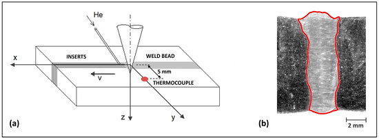
Figure 1.
Experimental welding process: (a) scheme of the welding setup; (b) macrograph of the welded cross-section and relief of fusion zone contour (red lines).
This welding setup has turned out to be particularly efficient, being easy to use, and able to compensate for geometric imperfections in the preparation of the plate edges and incidental errors in the alignment of the beam. Furthermore, by using a correct number of inserts, it allows one to limit the presence of welding defects, by avoiding the risk of incomplete fusion more easily than using filler wire [38].
The choice of AISI304L austenitic steel for the proposed application is due to the great interest in this type of material combined with fusion welding technologies, attributable to its wide use in constructions that are fabricated primarily by welding. Very recent literature confirms the persistent relevance of austenitic steels in applications based on laser welding [39,40,41]. Furthermore, the tendency of austenitic steels to undergo hot cracking during the last stages of solidification represents a serious issue in fusion welding. In particular, this phenomenon is affected by composition (Creq/Nieq ratio) and cooling rate. In this respect, the proposed theoretical model has proven to be a good tool to predict the solidification mode and properly select the welding parameters [32,33].
The laser beam quality, depending on the degree of focusing, and the diameter and position of the focus, has been evaluated by means of a diagnostic system, in order to establish the optimal operating parameters. The power P, welding speed v, focus diameter ϕf, and distance from the upper surface of the plates Δz are reported in Table 1.

Table 1.
Process welding parameters.
At these operating conditions, the incident beam energy is so high that the “keyhole” welding mode occurs, with the typical narrow cavity due to metal vaporization, surrounded by molten metal. The control of plasma, which is formed by the partial ionization of the vapor at high temperature, and can reduce beam energy absorption and prevent vaporization when temperature exceeds a critical value, has been obtained by a helium flow, directed towards the zone of interaction between the laser beam and the molten bath (the helium flow rate qHe also is reported in Table 1).
Macrographic observations of some cross-sections cut along the weld bead were performed using a stereo microscope, Leica MZ 16 1FA (Leica Microsystem, Milan, Italy). The cross-section surfaces were subjected to mechanical grinding (abrasive paper gradation from 180 to 2400), polished with a velvet cloth (aqueous suspension of Al2O3 with granulometry of 0.5 μm), and etched with glyceregia reagent (16% HNO3, 42% HCl, 42% glycerol). The results show a full penetration of the melt pool along the whole plate’s thickness (Figure 1b). The fusion zone (FZ) thus obtained is characterized by a regular shape, approximately 2 mm wide, with a flare towards the external surface at the beam side, and a certain enlargement in correspondence to the focus position. The micrographs show a base material microstructure consisting of recrystallized austenitic grains with average size of about 20 μm; the fused zone presents austenitic homogeneous dendrites with residual ferrite in tortuous and narrow interspaces, less than 1 μm thick [33].
To verify the robustness of the theoretical model regarding the fluctuations in the cross-sectional profile of the weld bead along the welding line, a specific analysis has been developed, comparing the effect that the geometric peculiarities of 5 cross-sections experimentally detected along the welding line has on the fitting of the model [31]. The substantial stability of the simulated thermal field, by varying the cross-section used for fitting the model parameters, have been verified, highlighting that the setting of the theoretical model is such as to make it insensitive to limited geometric variations in the cross-section; this ultimately confirmed the reliability of the model regardless of the specific weld bead profile on which it is fitted, at least in the case of welded joints with a substantially uniform shape, such as those obtained in the case of automatized laser welding.
The detection of the thermal cycle by thermocouple measurement, to be used for the experimental validation of the corresponding results obtained through the theoretical model and numerical simulation, was carried out, acquiring a single measurement by means of a K-type thermocouple (chromel/alumel, tolerance class 2, temperature range between −40 and 1200 °C, error 0.75%) spot welded on the upper surface of the plate, at a distance of 5 mm from the welding line (as indicated by the red dot in the setup scheme of Figure 1a). This type of experimental approach, based on a single measurement for each detection point, conforms to a consolidated practice in the acquisition of thermal cycles generated by welding processes at high energy density and speed [42,43]. In the proposed case, the single measurement point has been set at the maximum value of the distance from the welding axis within the range analyzed by theoretical modelling and numerical simulation (2–5 mm). This was necessary due to the limited space available to position the thermocouple as precisely as possible on the surface of the plate near the weld, considering the following factors: on the upper surface, the weld bead detected experimentally has the greatest width, which can exceed 2 mm on each side of the welding line; a main limitation in thermocouple placing is spattering near the welding line, particularly plentiful in the keyhole laser welding mode, at high power and speed.
2.2. Analytical Modelling of the Thermal Field
The conductivity-based model developed for the analytical calculation of the thermal field has been generalized to simulate all the cases that may occur in high power beam welding, including the deep penetration keyhole mode, by using the basic solutions for moving point and line heat sources [13]. This requires the assumption of the following preconditions:
- Quasi-stationary state condition: the onset of the temperature distribution around each source becomes rapidly constant, so that an observer fixed to the source does not detect temperature changes around it during its movement;
- Boundary conditions: the solid is assumed to be an infinite medium, not bounded by planes orthogonal to the motion direction; instead, boundaries can be assumed in terms of semi-infinite and finite thickness, which means that the solid may be bounded by one plane or delimited within two planes parallel to the motion direction; in both cases, no heat loss is assumed through the bounding planes;
- Incident point condition: the finite area of the real heat source is neglected, so the thermal field model drifts to infinite values of temperature at the beam incident point; this condition results in a lack of accuracy in the field simulation, which is greater the closer the calculation point is to the source.
To compensate for the simplification of the approach based on heat conduction only, the thermal field model needs to be configured as a virtual source system able to produce the same thermal effect of the actual laser welding process to be simulated. This effect is assumed to be expressed by the shape of the weld cross-sections, i.e., the profile of the FZ on the plane orthogonal to the direction of source movement. The latter, therefore, is taken as a reference to fit the configuration of the virtual heat sources, by setting the parameters that characterize the source’s system: the geometric layout parameters, and the parameters that distribute the real beam power among the virtual sources. In order to simulate the effect of the real thermal source, the system of the virtual ones must be calibrated by varying these parameters so as to make the corresponding theoretical FZ contour coincide as much as possible with the real one, which is experimentally detected.
With these parameters, assuming T0 (K) as the room temperature, and considering a reference system (x, y, z) whose origin is fixed to the beam incident point that moves along the x axis with a speed v (m/s), and the z axis is directed along the thickness of the solid (Figure 1a), the generalized analytical model for the thermal field is defined by superimposing a line source and multiple point sources, and expressed by [31]
The second term in Equation (1) expresses the 2D field due to a line source along the z axis, which can simulate the thermal effect of a uniform deep penetration welding. It includes the zero-order modified Bessel function of the second kind K0, and depends on the line source strength per unit length QL (W/m), the conductivity k (W/mK), the diffusivity α (m2/s), and the radial distance rL (m) from the heat source in the xy plane:
The third term in Equation (1) expresses the summation of 3D fields due to n point sources, which can simulate the effects of superimposed thermal fields with hemispherical or spherical shapes (on the surface of the solid body, or inside it, respectively), so as to adjust the uniformity of the field due to the line source and adapt it to the real non-uniform field actually generated by the deep penetration welding. This term depends on the strength of the point sources QPi (W), and the radial distance from each point source rPi:
where zPi is the depth of the i-th point source location along the z axis of the reference system. The numerical constants ci in Equation (1) can take on the value 2 or 4, if the i-th point source is located on the surface of the solid (zPi = 0), or inside the solid (zPi > 0), respectively.
The length of the line source along the z axis (zL), and the number (n) and location depth of the point sources on the same axis (zPi), define the layout of the model, and are the geometric layout parameters of the virtual sources system to be fitted on the real weld cross-section. The other set of parameters to be fitted, which define the thermal power distribution among the virtual sources of the system, are the coefficient γL and γPi that appear in the expressions of QL and QPi, respectively:
where P is the laser beam power (W), η is the absorption coefficient, and the condition γL + ΣγPi = 1 must be respected.
In the case under consideration, described in Section 2.1, the thermal analysis has been carried out by a field model based on the superimposition of one line source and two point sources; therefore, the model is expressed by Equation (1) with n = 2.
To simulate the effect of full penetration keyhole, reproducing the experimental profile of the FZ as accurately as possible, the geometric layout parameters have been predetermined according to the morphology of the FZ profile experimentally detected in the welded section and marked in Figure 1b:
- The line source has been extended along the whole bead thickness (zL = 10 mm), forming a full penetration FZ of uniform shape along the z axis;
- The two point sources have been located on the external surface at the laser beam side (zP1 = 0 mm), and inside the bead where the beam is focused (zP2 = Δz = 5.5 mm), giving rise to the convexities that characterize the experimental contour.
Therefore, in this case, the parameters of source’s strength distribution γL and γPi, and the absorption coefficient η in Equation (4), are the variables for fitting the FZ profile calculated by the analytical model (1) on the experimental FZ contour.
With this latter aim, a theoretical 3D model of the melt pool has been constructed by applying Equation (1) to obtain the isothermal curves at the solidus temperature (TS = 1673 K) on xy planes at different values of z (Figure 2a). Subsequently, the theoretical contour of the FZ on the cross-section of the joint bead has been obtained by projecting the boundaries of maximum amplitude of the 3D model of the melt pool (the melt pool track line in Figure 2a) onto a plane orthogonal to the moving axis x. For the calculations, in Equation (1), constant values have been assumed for the thermophysical properties of the AISI 304L steel, corresponding to an intermediate temperature equal to 700 °C [44]: thermal conductivity k = 25 W/mK, diffusivity α = 5.42 × 10⁻⁶ m2/s.
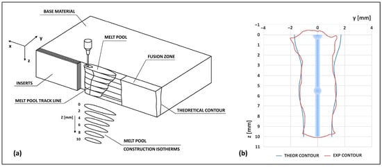
Figure 2.
Theoretical model fitting: (a) 3D model of the melt pool with scheme of the construction isotherms, and projection of the FZ cross-section contour; (b) fitting by comparison between the calculated and experimental contours of the weld bead cross-section (the three virtual thermal sources are symbolically reported).
Figure 2b shows the final comparison between the calculated FZ contour (the three virtual thermal sources configured to obtain it are illustrated also), and the contour relief of the cross-section of the experimental weld bead (Figure 1b). The fitting between the theoretical and the experimental contours has been performed by varying the previously defined parameters of the analytical model to minimize the sum of the squared distances along the y axis between the contours at different depths along the z axis. As a result, the coefficient of strength distribution among the sources (γL = 0.81, γP1 = 0.10, γP2 = 0.09) and the absorption coefficient (η = 0.51) of the virtual heat source system has been defined, the latter being in agreement with indicative data reported in the literature [45,46].
2.3. Multi-Physics Numerical Simulation
The generalized multipoint-line heat source model for the analytical calculation of the thermal field, described in Section 2.2, must be adapted to the specific case to be analyzed, by means of a fitting procedure based on geometric features of the experimental bead cross-section. The underlying assumption of this phenomenological approach is to simulate the factual thermal effect of deep penetration laser welding, also in the case of keyhole mode, by using a theoretical model based on the physical phenomenon of conductivity only, without evaluating the complex multi-physics processes that really occur.
To verify this assumption and validate the proposed theoretical approach and its analytical modelling, a full multi-physics numerical simulation that combines the main physical phenomena occurring in the actual keyhole mode welding process must be performed, so as to allow the comparison between the thermal fields obtained on the workpiece by the two different approaches.
The starting conceptual structure for the development of a simulation model in this field includes the implementation of the basic physical principles (energy, mass, and momentum conservation), complemented by models specifically developed to describe the interaction mechanisms between the laser beam and the material [25]. An adequate simulation tool must then be structured so as to include a solver of the equations that govern the basic physical principles, and additional modules to manage the specific physical phenomena involved.
A synthetic description of the keyhole phenomenon can help in identifying the physical models to be implemented in the numerical simulation [31].
With high-energy intensity laser beams, vaporization of the metal surface occurs, and the narrow cavity forms. The beam rays entering the cavity are scattered, and are partly absorbed on the walls of the keyhole, and partly reflected towards other points on the walls. This multiple absorption/reflection phenomenon increases the energy absorption, and results in high pressure and temperature of the metal vapor inside the keyhole.
The vapor that fills the keyhole cavity damps the beam, absorbing some of the incoming laser beam, which transmits kinetic energy to the particles in the vapor. When the kinetic gain is significant, the ionization of the metal vapor generates plasma. The latter has a beneficial effect on the stabilization of the keyhole, as it protects the cavity from cooling, and strengthens the vaporization at the inner walls. Nevertheless, as its temperature increases due to further ionization of the metal vapor, and exceeds a critical value, the beam damping effect becomes dominant and vaporization ends. The action of the shield gas is aimed precisely at controlling the plasma to stabilize the keyhole.
The metal vapor that flows out of the cavity, being replaced by newly evaporated material, generates a upward vapor pressure, with melt-flow ejection that carries away from the interaction zone a portion of the absorbed laser intensity, and can form a plume which causes further beam damping, and in some cases, defocusing, too.
All these effects combined together, also conflicting with each other, constitute an overall multi-physical mechanism, which creates and stabilizes the keyhole, and determine a thermal field, which will shape the cross-section of the FZ.
Here, the FLOW-3D® software package (Flow Science Inc., Santa Fe, NM, USA) has been used for the multi-physics simulation. The solution of the governing equations is performed by the primary CFD module FLOW-3D 12.0, which operates using the Finite Volume (FV) approach [47], and manages the free surfaces and the interfaces between different fluids by means of the Volume of Fluid (VOF) method [48].
The basic physical principles for laser welding simulation are governed by the conservation equations of continuity, momentum, energy, and mass fraction, and the heat transport equation, according to the formulations usually reported in the literature [5]. Furthermore, the process is implemented by using a set of standard physical models: heat transfer, solidification, vaporization (required for high power laser welding), density evaluation (required when volume changes due to density variations cannot be neglected), surface tension (required for deep penetration welding). The main forces acting in the models are buoyancy force, gravity, surface tension, and Marangoni convection.
The following additional physical models, required in the application to be simulated here, have been included by means of the FLOW-3D Weld 3.0.1 module, specifically dedicated to the simulation setup of welding processes:
- Heat source: The process parameter in Table 1 have been used for the basic heat source setting. The spatial configuration of the laser beam has been modelled with a cylindrical shape; the radius of the lens and laser spot radius (i.e., the radius at the focal plane) have been set as equal (0.25 mm according the data in Table 1). The Gaussian distribution has been set for the heat flux due to the source, so as to take into account that the energy density gradually attenuates from the center to the outside [49]. The value of 0.2 mm has been set for the radius of the inflection point, just above the value corresponding to the normal distribution (0.176 mm). This was necessary to guarantee a discretization of the heat flow distribution congruent with the mesh cell size that was set (as specified below).
- Evaporation pressure: The model is based on two evaporation pressure coefficients that are automatically calculated as a function of the material properties. The effect of the upward vapor pressure is included, and defined by a pressure magnification factor and the rising pressure radius, which correspond to the expected mean radius of the keyhole, assessed at 2 mm by using the calculation model of Rai et al. [50].
- Shield gas pressure on the free surface: this model has been set by defining the density of the He gas (0.1784 Kg/m3), and the velocity of the flow (5 m/s, calculated from the flow rate in Table 1, for a nozzle diameter of 9 mm).
- Multiple reflection and energy absorption mode: In this model, the constant absorption rate mode has been set, excluding angle-dependent mechanisms and Fresnel reflection. The reflections of the beam inside the keyhole continues until the residual energy density of the reflected ray reaches an attenuation rate limit. For the reasons that will be specified below, the result obtained by the fitting of the analytical model (η = 0.51) has been used to set the value of the absorption coefficient.
To reduce the computational load, the “half model” approach has been used in the definition of the analysis domain, exploiting the symmetry of the phenomenon with respect to the xz plane (Figure 3). The boundary conditions setting has been based on the configuration mode of the analysis domain, constituted by two mesh blocks:
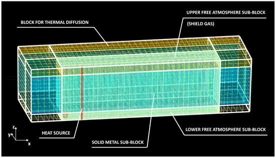
Figure 3.
Modelling and meshing of the analysis domain.
- The first mesh block is in turn divided into three sub-blocks: the central sub-block represents the portion of solid metal on which the action of the thermal source and its effects are simulated; the upper and lower sub-blocks, which interface, respectively, with the upper and lower surfaces of the central solid metal sub-block, have the properties of free atmosphere (1 atm pressure and room temperature equal to 293 K); the upper sub-block is also defined as the region in which the shield gas acts.
- The second mesh block is a surrounding outer block for thermal diffusion, which allows one to take into account the diffusion from the first block, in which the phenomenon is simulated, to the surrounding matter, not directly subjected to the process. Its extension is defined on the basis of the thermal diffusion distance, calculated as a function of the thermophysical properties of the medium (thermal conductivity, density, and specific heat), and of the simulation time.
In this configuration, the second mesh block constitutes a sort of overall boundary condition for the entire first mesh block. For this reason, the boundary conditions imposed on the first mesh block are “symmetry-type” conditions: they constitute simple interblock boundaries between the first block and the second one, which entirely incorporates the former. Inside the first block, the upper and lower sub-blocks impose boundary conditions on the central solid metal sub-block: atmospheric pressure and room temperature.
The following boundary conditions have been imposed on the limit planes of the second mesh block, defined with reference to the xyz coordinate system in Figure 3: for the limit planes at xmin, xmax, and ymax, the “wall-type” boundary condition with room temperature is applied (no fluid flow across the wall); for the limit planes at ymin, the “symmetry-type” boundary condition is applied (to simulate a virtual continuity with the second half of the analysis domain, which is symmetric with respect to the xz plane, and has been excluded from the model); for the limit planes at zmin and zmax, the “specified pressure-type” boundary condition with atmospheric pressure and room temperature is applied. The whole set of boundary conditions are summarized in Table 2.
Table 2.
Setting of boundary conditions (with reference to the configuration of the analysis domain shown in Figure 3).
In Figure 3, the heat source is represented by the vertical red cylinder extended along the thickness of the whole mesh blocks set.
The mesh cell size of the central block and the upper and lower atmospheric volumes has been set to 0.2 mm. This value must constitute a good compromise between the meshing accuracy and the calculation load. As a basic condition, to assure that the cells can capture effectively the discretized heat flux distribution of the beam, the cell size must not exceed the radius of the inflection point of the Gaussian distribution (0.2 mm). Furthermore, the accuracy of the domain meshing has been verified by an estimation of the error of the simulated laser power, which depends on the combination between the mesh cell size, the laser spot radius, and the radius of the inflection point of the heat flux distribution. This error turned out to be equal to −0.46%.
The mesh cell size of the surrounding thermal diffusion block has been defined by setting the ratio referring to the cell size of the solid metal block (1:5). For this block, a coarser mesh is allowable since its only function is to capture thermal diffusion.
The main thermophysical properties of the material (density, viscosity, specific heat, thermal conductivity, surface tension) have been set in tabular form to take into account their variation with the temperature. The data used to fill in the tables have been derived from the literature [44].
Finally, with regard to the key issue of setting the absorption coefficient, the data available in the literature for keyhole mode laser beam welding of steels [45,46] outline a very wide range of values, η = 0.50–0.80, which can allow for a rough orientation, but cannot provide sufficient indication to define a reliable value to be used in the numerical simulation. A calculation model expressly defined to estimate the absorption coefficient in the presence of keyholes, with reference to the case of some specific materials, including 304L stainless steel [50], allows one to obtain the value η = 0.55. As a further question to refine this estimation, it should also be considered that the assessment of absorption should concern only the portion of laser radiation that actually enters the keyhole, and that the wings of the radiation distribution have to be considered not intense enough to melt the material and so is reflected by the surface. As a consequence, a further reduction of about 6–10% in laser power must be considered in the case of steels [46], thus obtaining for the net absorption coefficient η a range of values between 0.49 and 0.52, which validate the result obtained by analytical model fitting (η = 0.51). The latter, therefore, has been set as the value of the absorption coefficient in the numerical model too.
3. Results and Discussion
3.1. Morphological Features of Keyhole Effects
Preliminary to the analysis of the thermal field, some observations on the evolution of the morphological characteristics of the melt pool and the consequent FZ appear to be particularly explanatory of the basic differences between the two compared approaches. Furthermore, the analysis of the shape features of the weld bead obtained through the numerical simulation, and their comparison with those detected experimentally, will be focused on as a preliminary factor for the validation of the numerical model.
Figure 4 and Figure 5 show some simulation results of the formation and stabilization of the melt pool and FZ during the first transitory stage of the keyhole. Three main types of results have been reported: the temperature distribution, the solid fraction, and the melt region. The last two are referred to in the xz plane, and are expressed in terms of the fractions of unity. In the case of the solid fraction, the unit value indicates the instantaneous distribution of the material in the fully solid state, while the zero value indicates the distribution of the material in the fully liquid state. In the case of the melt region, the unit value indicates the distribution of material which, up to the instance in question, has been subjected to melting. This material has partly assumed its final shape upon the completion of solidification, partly is still in a state of full or partial fusion, and has yet to assume its definitive shape once solidification is complete. The melt region in the state of complete solidification constitutes the FZ of the weld beam.
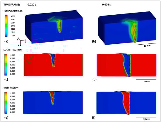
Figure 4.
Simulation results for keyhole formation during deep penetration laser welding at 20 ms and 74 ms: (a,b) 3D simulations of keyhole and temperature distributions; (c,d) solid fractions in xz plane; (e,f) melt regions in xz plane.
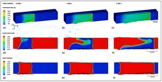
Figure 5.
Simulation results for keyhole transitory effects during deep penetration laser welding at 0.5, 1.0 and 1.5 s: (a–c) 3D simulations of keyhole and temperature distributions; (d–f) solid fractions in xz plane; (g–i) melt regions in xz plane.
Figure 4 shows the state of the keyhole formation at 20 ms from the start of the welding process, and the onset of full penetration after about 74 ms. In this case, the distributions of the solid fractions (Figure 4c,d) and melt region (Figure 4e,f) provide substantially the same information, as not enough time has yet passed for part of the molten material to have solidified and created a stable and consolidated portion of the melt region.
Figure 5 shows the transition phase, during which the keyhole and its effects evolve until they have stabilized, after approximately 1.5 s of process time. The evolution of the solid fraction in the time interval under examination (0.5 s to 1.5 s) highlights a clear tendency for the material affected by the keyhole to delay solidification in the lower region, resulting in an accumulation of liquid material (Figure 5d,e). This fluid dynamic behavior has already been observed previously, and attributed to the formation of waves of liquid melt, known as keyhole humps [51,52], running along the keyhole front, down to the end of the melt pool, which grows under the effect of turbulence in the lower rear part, until reaching a stable extension [53]. The latter condition is shown in Figure 5f, with a final extension of the lower accumulation wake of the melt pool equal to approximately 30 mm.
The melt region, the progression of which in the xz plane is shown in Figure 5g–i, is affected by the morphological evolution of the solid fraction, as previously described. Of particular interest here are the cross-sections on the planes parallel to yz, which, when referring to the melt region in the state of complete solidification, constitutes the FZ cross-sections of the weld beam. Figure 6a,b show the fully solidified melt region on the xz plane, and the evolution of the corresponding FZ cross-sections along the weld bead, respectively, with regard to the transient phase represented in Figure 5, in the 0.5–1.5 s interval of the process time. The latter corresponds to the distances from 10 mm to 30 mm with respect to the starting point of the process (the welding speed being set at 1.2 m/min).
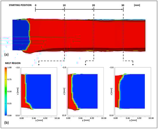
Figure 6.
Simulation results for FZ cross-section evolution from starting point to stabilization: (a) fully solidified melt region on the xz plane; (b) evolution of corresponding FZ cross-section (xy plane) along the weld bead.
The evolution of the FZ cross-sections is strictly related to the solid fraction one (Figure 5d–f): at 10 and 20 mm from the starting point (process time equal to 0.5 s and 1.0 s, respectively), the effect of liquid material accumulation in the lower melt pool causes the large flaring of the FZ cross-section in the lower part of the weld bead. In the subsequent increase in the distance of 20 mm up to 30 mm (process time from 1.0 s to 1.5 s), the lower accumulation wake of the melt pool lengthens in the x direction until it stabilizes, and at the same time, thins in the y direction. As a consequence, an inversion of the morphological characteristics of the FZ cross-section occurs (last frame in Figure 6b), with a flare that stabilizes in the upper part of the weld bead, and the lower part that reduces and becomes uniform in width.
This last morphology of the FZ can be considered stationary, since the transitory phase of the keyhole effects is completed at the end of the analyzed interval, and starting from the 30 mm cross-section, the morphological effects of the phenomenon can be considered stabilized. Therefore, it can be assumed as the reference FZ cross-section of the numerical simulation, and compared to the experimental and theoretical ones (Figure 7).
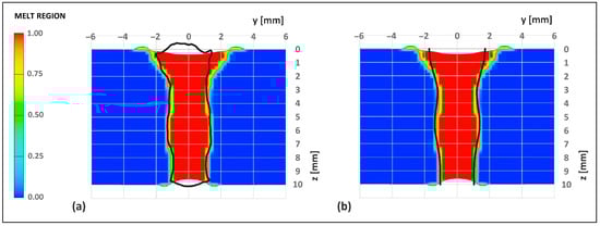
Figure 7.
Comparison between the contours of FZ cross-section: (a) numerical simulation vs. experimental detection (black lines); (b) numerical simulation vs. theoretical calculation (black lines).
From a first general observation, in both comparisons, it is possible to notice a close affinity between the FZ contours, with an evident sharing of the main morphological traits: the upper flaring (that forms the typical “nail head” at the top of the weld), and a progressive homogenization of the width in the development along the z axis, in which the slight expansion is noted in correspondence with the position of the laser focus. In fact, the contours are superimposable, with the exception of the upper part, which, in the result of the numerical simulation, presents a markedly wider flare, both compared to the experimental detection and the result of the theoretical calculation.
To quantify the overall affinity between the contours to be compared, the same metric used for fitting the analytical model on the basis of the experimental one has been used: the sum of the squared distances along the y axis between the contours, measured at four different depths along the z axis (z = 1, 3.5, 6, 8.5 mm), has been calculated; considering the difference between the left (−y) and right (+y) contour of the experimental FZ, the calculation of the sum of the squared distances has been specifically differentiated; as a further option in the distances calculation, the average value of the width of the two experimental semi-contours has been also used.
The results of the affinity assessment are reported in Table 3. The lower the values of the chosen metrics, the greater the affinity between the contours.
Table 3.
Affinity between the contours of FZ cross-sections expressed by the sum of the squared distance (control points at z = 1, 3.5, 6, 8.5 mm).
In the comparison between the experimental and numerical contours, the values highlight a high affinity between the −y contours, which are perfectly superimposable, and a reduction in the case of the +y contours, clearly attributable to the deviation in the shapes of the upper flare on the right side. The data obtained with respect to the average value of the experimental +y and −y contours provides an intermediate affinity evaluation between the two previous ones. On the whole, the affinity between the contours of the numerical and experimental FZ cross-sections is high, which validates the settings and results of the numerical model, proving it to be well-calibrated.
The affinity between the experimental and theoretically calculated contours appears to be significantly better when compared to the previous case (the values of all metrics are substantially lower). This is a direct consequence of the setting of the theoretical model, which required the fitting of the characterizing parameters precisely through the minimization of the deviations between the experimental and theoretical contours.
Finally, the assessment of the affinity between the theoretically calculated contours and the ones obtained from the numerical simulation has been also included in Table 3. In this case, given the symmetry of both contours, there is no difference between the left and right sides, nor does it make sense to use averaged values. The value of the metric is therefore unique, confirming also in this case the high affinity between the two results compared.
As a final observation on the morphological features related to the keyhole effects, the comparison between the contours of the melt pool obtained by the numerical simulation and analytical calculation is significant. The theoretical 3D model of the melt pool can be constructed by means of the isothermal curves at the solidus temperature on the xy planes at different values of z, as described in Section 2.2, and schematized in Figure 2a. The result obtained is shown in Figure 8, where the theoretical contours of the melt pool in the xz plane (white lines) have been superimposed on the solid fraction distribution simulated by the numerical modeling in stabilized conditions (Figure 5f). The latter can outline the contours of the melt pool, if the boundaries that include the areas associated with the color gradations closest to the zero value are considered. As a result of the comparison, the substantial convergence of the two models on the estimate of the extension of the melt pool near the upper surface of the workpiece, equal to approximately 13 mm (including the contribution due to the front region), is noteworthy.
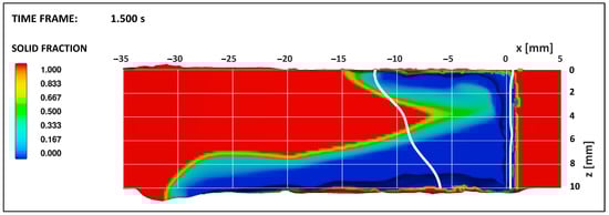
Figure 8.
Comparison between the contours of melt pool in xz plane: numerical simulation vs. theoretical calculation (white lines).
Moving away from the upper surface, inside the workpiece, the two models diverge sharply. This highlights the intrinsic limitation of models that do not take into account the fluid dynamics of the phenomenon, and cannot capture the effects previously described, at the origin of the distribution of the solid fraction shown in the figure, with particular regard to the lower rear region of the melt pool. The discrepancy in the results regarding the front profile of the melt pool is also attributable to the missing fluid dynamic phenomena contribution in the analytical model, with specific reference in this case to the phenomenon of the keyhole humps, introduced earlier.
In the end, a substantial inadequacy of the analytical modeling based exclusively on thermal conduction, in predicting the shape of the melt pool, clearly emerges. Only near the surface, where the beam–matter interaction occurs first (z = 0), the analytical estimate of the size of the melt pool provides information that converges with the multi-physics numerical model. This suggests that, in this specific region, a condition occurs in which the phenomenon of thermal conduction is prevalent. This can be explained in terms of the conduction-to-keyhole transition [54]: as long as the phenomenon of the multiple reflection of the laser beam is limited, and is not enough to trap a significant fraction of incident rays inside the cavity, as happens in the region closest to the external surface of the solid body, the transition to the keyhole mode cannot be considered to have occurred locally, and the thermal behavior is limited to the conduction mode. The pronounced flare that characterizes the morphology of the upper FZ cross-section, in both cases of experimental detection and numerical simulation, as highlighted previously (Figure 7), confirms the prevalence of the conduction mode, limited to this specific region. Moving away from the upper surface, through the solid body, the other physical phenomena typical of the keyhole mode emerge and become decisive, leading to evolutions of the shape of the melt pool that are completely divergent compared to the simplification of the conductivity-based model.
3.2. Thermal Field in the Workpiece
Once the analytical model introduced in Section 2.2 has been fitted, various simulations to evaluate the thermal effects of the mobile heat source can be performed. As an expression of the thermal field, the temperature–time curves for the fixed points on the solid body are particularly significant, as they form the basis for various predictive investigations on the properties of the welded joint (the composition, solidification mode, microstructure of weld bead, residual stress distribution and distortion). These curves can be obtained by Equation (1) if a coordinate transformation is introduced.
As a matter of fact, Equation (1) allows for the calculation of the thermal field due to the virtual heat source in each point (x,y,z) of the solid body, according to the reference system fixed on the moving source (Figure 1). As a consequence, the corresponding value of the temperature is invariant with time, since the position of the point (x,y,z) with respect to the source is also invariant. To analyze the temperature cycles in a fixed point of the solid body as time varies, it is necessary to take into account the variation in the distance between the point and the mobile source due to the movement of the latter. This can be achieved by applying the following coordinate transformation to Equation (1):
where v is the moving speed of the heat source along the x axis, and t is the time. In this way, a fixed point on the workpiece, with respect to the mobile reference system xyz, is identified by the coordinates (ξ,y,z).
The temperature–time curves for the fixed points on the plane xy, at z = 0 mm (that is, the beam side surface of the workpiece), obtained by means of x ξ transformation (5), are shown by solid lines in Figure 9 for different distances y from the welding axis, starting from y = 2 mm up to y = 5 mm, and, therefore, outside the FZ (the boundary of which at z = 0 mm, defined by the same theoretical model, results in y = 1.73 mm). Each curve shows the thermal profile of a point fixed on the surface of the workpiece, and located along a line orthogonal to the welding axis. The profiles are extended for a process time equal to 10 s. The corresponding values of the distance ξ (mm) between the detection point and the thermal source along the x axis, for each time t (s), that is, the welding length at time t, are calculated using the coordinate transformation (5), and reported on the abscissa axis of the graph. In the same figure, the curves corresponding to the thermal profiles obtained through the numerical simulation are also shown with dashed lines.
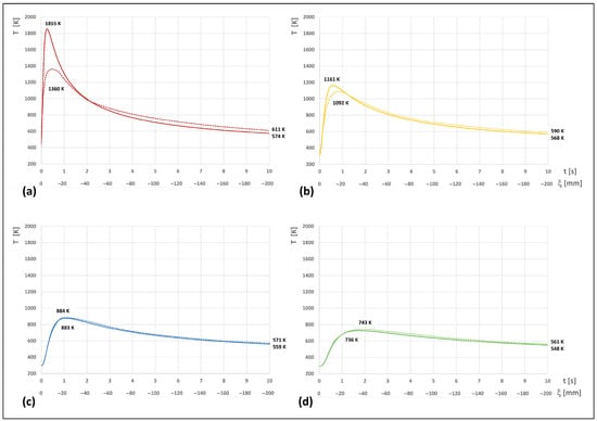
Figure 9.
Comparison between theoretical and numerically simulated thermal profiles (solid and dashed lines, respectively) in fixed points on the surface of the workpiece (z = 0 mm), for process time of 10 s (welding length equal to 200 mm), varying the distance y of the point from the welding line: (a) y = 2 mm; (b) y = 3 mm; (c) y = 4 mm; (d) y = 5 mm.
To appreciate in detail the comparability of the theoretical and numerical results, in Figure 9, the theoretical thermal profile for each of the four points analyzed (y = 2, 3, 4, 5 mm) is coupled to the corresponding profile obtained through numerical simulation (solid and dashed curves, respectively). The temperature values corresponding to the thermal peaks, and to the end of the analyzed time interval (t = 10 s), are reported.
Further quantitative details on the comparison, expressed by percentage variations in the numerical simulation vs. theoretical calculation values in the corresponding points of the curves, are reported in the top half of Table 4. Specifically, the following metrics of deviation have been assessed: the variation between the two maximum peak values (εp); the maximum variation in the second part of the curves (on the right side), which tends to stabilize according to a common trend (εsmax); the variation between the end values of the two curves, where t = 10 s (εt10).
Table 4.
Comparison between thermal profiles (at z = 0 mm and z = 5 mm): percentage variations in temperature values obtained by numerical simulation vs. theoretical calculation.
From the comparison of the pairs of curves, it is preliminarily possible to observe that, for y = 2 and 3 mm, the coupled curves are substantially superimposable, starting from the low values of the process time (about 1–1.5 s, i.e., distance from the heat source along the x axis equal to ξ = 20–30 mm), and for y = 4 and 5 mm, they are fully superimposable for the entire analyzed process time. At a greater level of detail, it is possible to outline the following further observations:
- For the points closest to the welding line (y = 2 and 3 mm), a theoretical overestimation of the temperature is evident in the first part of the curves (lower process times), in which the distance between the points and the moving thermal source is short with respect to the x axis. This aspect can clearly be traced back to one of the preconditions on which the analytical model with conductive thermal sources is based, introduced at the beginning of Section 2.2: due the assumption that the finite area of the real heat source is neglected, the thermal field drifts to infinite values of temperature at the beam incident point, resulting in a lack of accuracy in the field simulation, with an overestimation of the thermal values that is higher the closer the detection point is to the welding line. From a strictly mathematical point of view, this drift towards infinite values is inherent to the formulation of the terms in Equation (1) that express the thermal field generated by the point sources and the line source. When ξ → 0 (i.e., x → 0 and t → 0) and y → 0, meaning that the point to calculate the thermal field tends to position itself in correspondence with the same temporary position of the heat source, the term in Equation (1) for the point source on the surface (zP1 = 0) tends to infinity; the term for the line source tends to finite but off-scale values (furthermore, the argument of the Bessel function K0 that appears in this term tends to a zero value, which is not allowed as an argument to this function). This confirms the intrinsic lack of accuracy in the thermal field calculation for points very close to the temporary position of the heat sources, when using the Rosenthal formulation for conductivity-based thermal field modelling. As a result, the deviation of the peak values is very high for y = 2 mm (εp = −26.7%), and not negligible for y = 3 mm (εp = −5.9%). The drift in the theoretical calculation of the thermal field, already moderate in the case of the point at y = 3 mm, runs out completely, starting from y = 4 mm (εp < 1%).
- In all the points analyzed, after the temperature peaks, the coupled thermal profiles regularize into a similar decreasing trend that tends to stabilize, with a low value of percentage variation (εsmax and εt10 < 8% for y = 2 and 3 mm), and in some cases, with a substantial overlapping of the theoretical and numerical curves (εsmax and εt10 < 3% for y = 4 and 5 mm).
- As a further observation on the temperature decrease and stabilization phase, the comparison between the values of εsmax and εt10 can be significant: when the condition εsmax > εt10 occurs, this means that the two compared curves tend to converge further as the process time increases (what happens for y = 2, 3, 5 mm).
The thermal profile calculated using the analytical model for the point at y = 5 mm and z = 0 mm (Figure 9d) was subjected to experimental validation through a comparison with the thermal profile detected on the same point using a K-type thermocouple (see previous Section 2.1). The results have been reported in Figure 10, for a process time of 20 s, adding to the comparison the thermal profile obtained by the numerical simulation (dotted green line, limited to the process time of 10 s, at which the numerical simulation has been set in this study, to contain the long calculation times). The experimental profile obtained by the direct measurement acquired is reported as the dashed red line with the lower peak, and is delayed because of the thermocouple response time.
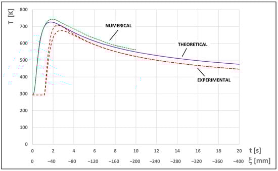
Figure 10.
Thermal profiles in the fixed point at y = 5 mm on the surface of the workpiece (z = 0 mm), for process time of 20 s (welding length equal to 400 mm): comparison between theoretical, numerical, and experimental profiles (direct and corrected measurements).
The key values of the deviations of the numerical simulation and theoretical calculation vs. experimental detection profiles have been reported in Table 5. They have been calculated considering the experimental profile shifted on the left to compensate for the delay in the detection time. The variation between the end values of the experimental and theoretical curves, where t = 20 s (εt20), has been added to the table. The estimate of εsmax was not relevant here.
Table 5.
Comparison between thermal profiles (z = 0 mm, y = 5 mm): percentage variations in numerical simulation and theoretical calculation vs. direct and corrected experimental measurements.
The theoretical profile appears to exceed the experimental one, with a maximum deviation at the peaks εp equal to 7%, and stabilizing deviations εt10 and εt20 equal to 6.2% and 6.0%, respectively. The numerical profile further exceeds the experimental one, with a maximum deviation at the peaks εp equal to 8.3%, and end point deviation εt10 equal to 7.9%.
The result of this first comparison with the direct experimental curve is in agreement with the evidence reported in the literature, revealing a clear trend, according to which the thermocouple measurements of the thermal cycles generated by the welding processes with high energy density and execution speed are usually underestimated compared to the results of numerical simulations [42,43].
This trend can be traced back to the level of accuracy of the measurement obtained by the thermocouple, which can be evaluated by analyzing the main errors of the measurement. As regards the specific application, and the thermocouple used, the following measurement error terms can be estimated:
- Intrinsic measurement error of 0.75% (from thermocouple technical specifications);
- Positioning error, due to positioning deviations with respect to the pre-established detection point, the extent of which is strictly dependent on the gradient of the thermal signal to be measured with respect to the distance from the welding line; in the application, a maximum error value of 1.5% for each tenth of a millimeter of deviation from the pre-set positioning point has been estimated;
- Response lag error, due to the inherent response lag of the thermocouple, which does not allow it to attain steady state measures since the instantaneous temperature changes very fast, particularly for heat sources with high energy density moving at high speed.
Considering the limited impact of the first two, the underestimation of the experimental measurement can be attributed to the third error factor, which can be corrected by formulations in the literature. The curve of the direct thermal signal with the correction of the response lag error proposed by Nayak et al. [43], which aims to compensate for the effect of the thermocouple response time constant, has been also reported in Figure 10 (dashed red line with the higher peak). Since the applied correction acts on the peak portion of the curve, its primary effect is to outline a better agreement between the experimental curve and the theoretical and numerical ones precisely in correspondence with the greatest deviation in the comparison with the uncorrected experimental curve. This is confirmed by the values assumed by the maximum deviations at the peak εp of both the numerical and theoretical curves vs. the corrected experimental one, which drops to 4.5% and 3.6%, respectively (Table 5, values in brackets).
As a result, the estimated deviation result is limited, being, on the whole, significantly less than 10%, and confirming an adequate level of accuracy for both the theoretical calculation and numerical simulation.
As a final verification of the congruence between the theoretical and numerical results, the thermal profiles in fixed points at the same distance from the welding axis as before, but located at the center of the workpiece’s thickness (z = 5 mm), have also been compared and collected together in Figure 11. The quantitative details expressed by percentage variations in the curves are reported in the bottom half of Table 4.
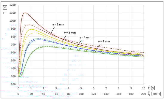
Figure 11.
Thermal profiles in fixed points at the center of the workpiece’s thickness (z = 5 mm), for process time of 10 s (welding length equal to 200 mm), parameterized according to the y coordinate (distance of the point from the welding line): theoretical calculations (solid lines) vs. numerical results (dashed lines).
In this case, compared to the results in Figure 9 (z = 0 mm), the thermal profiles present initially lower temperatures, as is evident from the values of the peaks. However, as the process time increases (i.e., the distances ξ of the detection points from the heat source increase), even in this case, a stabilization towards temperature values around 600 K occurs. This effect of reducing temperatures at the center of the plate, even if limited to the first phase of the heat source effect on the analyzed points, is congruent with the shape of the cross-section FZ both experimentally detected and simulated (Figure 7).
From a qualitative point of view, the trends of the pairs of the thermal profiles in Figure 11 are completely similar to those of Figure 9, for each value of y analyzed.
In particular, a common feature appears to be of interest in highlighting the substantial differences between the theoretical and numerical approaches. The temperature stabilization phase is always characterized by a reversal of the trend between the coupled curves, if compared to the first parts of the curves (before the stabilization start), with an overestimation, albeit limited, of the temperature profiles obtained through the numerical simulation, compared to the theoretical ones. This trend reversal is attributable to the different conditions that arise. For lower values of the process time (i.e., shorter distances between the detection point and the heat source) the inaccuracy of the analytical model due to the drift to infinite temperatures near the heat source prevails over any other condition, and this causes the overestimation of the thermal field obtained through the theoretical model. As the process time increases (and so does the distance between the detection point and the heat source), the trend reversal in the overestimation between the two curves is due to the prevalence of the effects due to thermophysical and fluid dynamic phenomena, modelled in detail by the multi-physics approach. In particular, it can be noted how these phenomena lead to a delay in the cooling and solidification of the molten metal (clearly shown by the evolution of the solid fraction in Figure 5d–f, already discussed previously). Therefore, it is reasonable to attribute the condition of the overestimation of the thermal curves obtained by the numerical simulation to this delay in material cooling during the thermal processes.
From the quantitative point of view, the data in Table 4 highlight a clear reduction in the deviation in the peak values εp for y = 2 and 3 mm, compared to the surface condition (z = 0 mm). On the whole, the percentage variations analyzed for z = 5 mm are lower than in the previous case. These latest results therefore confirm and strengthen a significant convergence between the theoretical and numerical data.
As a final consideration, excluding the inaccuracy of the analytical model when the detection point is in a position particularly close to the thermal source, the results of the theoretical calculations and numerical simulations are clearly convergent; therefore, the thermal field evaluated analytically can be considered validated by numerical simulation.
4. Conclusions
The new conduction-based and experimentally fitted parameterized model of the thermal field previously introduced has already undergone basic experimental validation, in the case of full penetration keyhole mode CO2 laser beam welding of AISI 304L austenitic stainless steel plates, with satisfactory results. To further strengthen the validation of the theoretical model, define its application limits, and assess the accuracy of its results, an extended investigation by means of a multi-physics numerical simulation, performed by the commercial CFD software package FLOW-3D, has been carried out.
With this purpose, the effects of the keyhole welding mode on the main morphological features of the melt pool and fusion zone, and the thermal fields obtained by the theoretical model and the numerical simulation, have been compared. The main results of the investigation can be summarized as follows:
- A limitation of the analytical modeling based exclusively on thermal conduction, in predicting the shape of the melt pool, clearly emerges. Only near the surface, where the beam–matter interaction occurs first, the analytical estimate of the size of the melt pool converges with the multi-physics numerical model. This suggests that, in this specific region, the phenomenon of thermal conduction is prevalent. Moving away from the surface, through the solid body, the other physical phenomena typical of the keyhole mode prevail, and the shape of the simulated melt pool becomes substantially divergent if compared to the one calculated by the conductivity-based model.
- For points on the surface of the plates closest to the welding line, a theoretical overestimation of the temperature is evident in the first part of the thermal cycles, in which the thermal peak occurs and the distance between the points and the moving thermal source is short. This aspect can be traced back to a loss of accuracy that is inherent in the analytical models based on conductive thermal sources, with an overestimation of the thermal values that is higher the closer the detection point is to the welding line. Instead, in all the points analyzed, after the temperature peaks, the thermal profiles regularize into a similar decreasing trend, with a substantial overlapping of the theoretical and numerical curves.
- For the point furthest from the welding line, among those analyzed on the surface, the thermal profiles calculated using the analytical model and the numerical simulation have been subjected to experimental validation. The result of a comparison with the thermal profile detected using a thermocouple is in agreement with the evidence reported in the literature, confirming a clear trend of the thermocouple measurements to be underestimated if compared to the results of both the other approaches, due to the response lag error of the thermocouple. However, a substantial convergence with the compared data occurs. This is improved by the correction of the direct thermocouple measurement, obtaining very limited deviations, and confirming an adequate level of accuracy for both the theoretical calculation and numerical simulation.
- The congruence between the theoretical and numerical results has been further verified by analyzing the thermal profiles in fixed points located at the center of the workpiece’s thickness. A marked overlapping of the theoretical and numerical thermal profiles and a clear reduction in the deviation in the peak values compared to the surface condition can be pointed out.
As final considerations, the results confirm a significant convergence between the theoretical and numerical data, and strengthen the validation of the thermal field calculated using the analytical model, apart from the loss of accuracy when the detection point is in a position particularly close to the movement path of the heat source. The limitations of the analytical simulation based only on the conductive phenomenon, in predicting the shape of the melt pool, have been instead outlined. The primary purpose of the validated theoretical model is confirmed to be that of predicting the thermal field. Used in the practice of laser welding applications, it can allow for a detailed evaluation of the thermal effects resulting from the setup of welding parameters, facilitating the selection of the optimal process conditions, and promoting a proactive welding process control.
Author Contributions
Conceptualization, F.G. and A.S.; methodology, F.G. and A.S.; software, F.G.; validation, F.G. and A.S.; formal analysis, F.G. and A.S.; investigation, F.G. and A.S.; resources, F.G. and A.S.; data curation, F.G. and A.S.; writing—original draft preparation, F.G. and A.S.; visualization, F.G. and A.S.; supervision, F.G. and A.S.; funding acquisition, F.G. All authors have read and agreed to the published version of the manuscript.
Funding
This research was partly funded by the University of Catania, Italy, within the plan “PIAno di inCEntivi per la Ricerca di Ateneo 2020/2022”, action line 3 “Starting Grant”, project “MESOTERMM—Modellazione degli Effetti di SOrgenti TERmiche mobili a elevata potenza sulle proprietà dei Materiali Metallici”, Department of Civil Engineering and Architecture.
Data Availability Statement
The data presented in this study are contained within the article.
Acknowledgments
The authors gratefully acknowledge Filippo Palo at XC Engineering Srl for the useful suggestions in implementing the numerical model.
Conflicts of Interest
The authors declare no conflict of interest. The funders had no role in the design of the study; in the collection, analyses, or interpretation of the data; in the writing of the manuscript; or in the decision to publish the results.
References
- Katayama, S. Fundamentals and Details of Laser Welding; Springer: Singapore, 2020. [Google Scholar]
- Volpp, J.; Laskin, A. Beam shaping solutions for stable laser welding: Multifocal and multispot beams to bridge gaps and reduce spattering. PhotonicsViews 2021, 18, 38–41. [Google Scholar] [CrossRef]
- Piwnik, J.; Szczucka-Lasota, B.; Wegrzyn, T.; Majewski, W. Laser welding with micro-jet cooling for truck frame welding. Transp. Probl. 2017, 12, 107–114. [Google Scholar] [CrossRef]
- Huang, Z.; Cao, H.; Zeng, D.; Ge, W.; Duan, C. A carbon efficiency approach for laser welding environmental performance assessment and the process parameters decision-making. Int. J. Adv. Manuf. Technol. 2021, 114, 2433–2446. [Google Scholar] [CrossRef]
- Nabavi, S.F.; Farshidianfar, A.; Dalir, H. A comprehensive review on recent laser beam welding process: Geometrical, metallurgical, and mechanical characteristic modeling. Int. J. Adv. Manuf. Technol. 2023, 129, 4781–4828. [Google Scholar] [CrossRef]
- Mackwood, A.P.; Crafer, R.C. Thermal modelling of laser welding and related processes: A literature review. Opt. Laser Technol. 2005, 37, 99–115. [Google Scholar] [CrossRef]
- Karkhin, V.A. Thermal Processes in Welding, 2nd ed.; Springer Nature: Singapore, 2019. [Google Scholar]
- Lindgren, L.-E. Finite element modeling and simulation of welding Part 1: Increased complexity. J. Therm. Stresses 2001, 24, 141–192. [Google Scholar] [CrossRef]
- Lindgren, L.-E. Finite element modeling and simulation of welding Part 2: Improved material modeling. J. Therm. Stresses 2001, 24, 195–231. [Google Scholar] [CrossRef]
- Lindgren, L.-E. Finite element modeling and simulation of welding Part 3: Efficiency and integration. J. Therm. Stresses 2001, 24, 305–334. [Google Scholar] [CrossRef]
- Marques, E.S.V.; Silva, F.J.G.; Pereira, A.B. Comparison of finite element methods in fusion welding processes: A review. Metals 2020, 10, 75. [Google Scholar] [CrossRef]
- Anca, A.; Cardona, A.; Risso, J.; Fachinotti, V.D. Finite element modeling of welding processes. Appl. Math. Model. 2011, 35, 688–707. [Google Scholar] [CrossRef]
- Rosenthal, D. The theory of moving sources of heat and its application to metal treatments. Trans. ASME 1946, 68, 849–866. [Google Scholar] [CrossRef]
- Carslaw, H.S.; Jaeger, J.C. Conduction of Heat in Solids; Oxford University Press: London, UK, 1959. [Google Scholar]
- Hekmatjou, H.; Zeng, Z.; Shen, J.; Oliveira, J.P.; Naakh-Moosavy, H. A comparative study of analytical Rosenthal, finite element, and experimental approaches in laser welding of AA5456 alloy. Metals 2020, 10, 436. [Google Scholar] [CrossRef]
- Dowden, J.M. The Mathematics of Thermal Modeling: An Introduction to the Theory of Laser Material Processing; Chapman & Hall/CRC: Boca Raton, FL, USA, 2001. [Google Scholar]
- Van Elsen, M.; Baelmans, M.; Mercelis, P.; Kruth, J.-P. Solutions for modelling moving heat sources in a semi-infinite medium and applications to laser material processing. Int. J. Heat Mass Transf. 2007, 50, 4872–4882. [Google Scholar] [CrossRef]
- DebRoy, T.; David, S.A. Physical processes in fusion welding. Rev. Mod. Phys. 1995, 67, 85–112. [Google Scholar] [CrossRef]
- Ki, H.; Mohanty, P.S.; Mazumder, J. Modeling of laser keyhole welding: Part I. Mathematical modeling, numerical methodology, role of recoil pressure, multiple reflections, and free surface evolution. Metall. Mater. Trans. A 2002, 33, 1817–1830. [Google Scholar] [CrossRef]
- Gong, S.; Pang, S.; Wang, H.; Zhang, L. Weld Pool Dynamics in Deep Penetration Laser Welding; Springer: Singapore, 2021. [Google Scholar]
- Cai, W.; Jiang, P.; Shu, L.S.; Geng, S.N.; Zhou, Q. Real-time laser keyhole welding penetration state monitoring based on adaptive fusion images using convolutional neural networks. J. Intell. Manuf. 2023, 34, 1259–1273. [Google Scholar] [CrossRef]
- Coviello, D.; D’Angola, A.; Sorgente, D. Numerical study on the influence of the plasma properties on the keyhole geometry in laser beam welding. Front. Phys. 2021, 9, 754672. [Google Scholar] [CrossRef]
- Kang, Y.; Zhao, Y.; Li, Y.; Wang, J.; Zhan, X. Simulation of the effect of keyhole instability on porosity during the deep penetration laser welding process. Metals 2022, 12, 1200. [Google Scholar] [CrossRef]
- Wang, C.; Mi, G.; Zhang, X. Welding stability and fatigue performance of laser welded low alloy high strength steel with 20 mm thickness. Opt. Laser Technol. 2021, 139, 106941. [Google Scholar] [CrossRef]
- Otto, A.; Koch, H.; Leitz, K.-H.; Schmidt, M. Numerical simulations—A versatile approach for better understanding dynamics in laser material processing. Phys. Procedia 2011, 12, 11–20. [Google Scholar] [CrossRef]
- Svenungsson, J.; Choquet, I.; Kaplan, A.F.H. Laser welding process: A review of keyhole welding modelling. Phys. Procedia 2015, 78, 182–191. [Google Scholar] [CrossRef]
- Volpp, J.; Vollertsen, F. Keyhole stability during laser welding-part I: Modeling and evaluation. Prod. Eng. Res. Dev. 2016, 10, 443–457. [Google Scholar] [CrossRef]
- Steen, W.M.; Dowden, J.; Davis, M.; Kapadia, P. A point and line source model of laser keyhole welding. J. Phys. D Appl. Phys. 1988, 21, 1255–1260. [Google Scholar] [CrossRef]
- Dowden, J.; Kapadia, P. Point and Line Sources: Models of Power Absorption in the Theory of Welding. In Proceedings of the ICALEO ’98 Laser Materials Processing Conference, Orlando, FL, USA, 14–18 October 1998. [Google Scholar] [CrossRef]
- Franco, A.; Romoli, L.; Musacchio, A. Modelling for predicting seam geometry in laser beam welding of stainless steel. Int. J. Therm. Sci. 2014, 79, 194–205. [Google Scholar] [CrossRef]
- Giudice, F.; Missori, S.; Sili, A. Parameterized multipoint-line analytical modeling of a mobile heat source for thermal field prediction in laser beam welding. Int. J. Adv. Manuf. Technol. 2021, 112, 1339–1358. [Google Scholar] [CrossRef]
- Giudice, F.; Sili, A. Weld metal microstructure prediction in laser beam welding of austenitic stainless steel. Appl. Sci. 2021, 11, 1463. [Google Scholar] [CrossRef]
- Giudice, F.; Sili, A. Investigation on laser beam weldability of AISI 304L plates based on thermal field simulation by experimentally-fitted analytical modeling. Lasers Manuf. Mater. Process. 2021, 8, 466–490. [Google Scholar] [CrossRef]
- Giudice, F.; Sili, A. A theoretical approach to the residual stress assessment based on thermal field evaluation in laser beam welding. Int. J. Adv. Manuf. Technol. 2022, 123, 2793–2808. [Google Scholar] [CrossRef]
- Kik, T. Heat source models in numerical simulations of laser welding. Materials 2020, 13, 2653. [Google Scholar] [CrossRef]
- Taylor, G.A.; Hughes, M.; Strusevich, N.; Pericleous, K. Finite volume methods applied to the computational modelling of welding phenomena. Appl. Math. Model. 2002, 26, 311–322. [Google Scholar] [CrossRef]
- De, A.; DebRoy, T. Improving reliability of heat and fluid flow calculation during conduction mode laser spot welding by multivariable optimization. Sci. Technol. Weld. Join. 2006, 11, 143–153. [Google Scholar] [CrossRef]
- Missori, S.; Sili, A. Prediction of weld metal microstructure in laser beam weld metal clad steel. Metallurgist 2018, 62, 84–92. [Google Scholar] [CrossRef]
- Drobniak, P.; Otto, A.; Gómez Vázquez, R.; Arias, R.M.; Arias, J.L. Simulation of keyhole laser welding of stainless steel plates with a gap. Procedia CIRP 2020, 94, 731–736. [Google Scholar] [CrossRef]
- Evin, E.; Tomáš, M. Formability prediction of laser-welded stainless steel AISI 304 and AISI 430. Metals 2022, 12, 54. [Google Scholar] [CrossRef]
- Diegel, C.; Mattulat, T.; Schricker, K.; Schmidt, L.; Seefeld, T.; Bergmann, J.P.; Woizeschke, P. Interaction between local shielding gas supply and laser spot size on spatter formation in laser beam welding of AISI 304. Appl. Sci. 2023, 13, 10507. [Google Scholar] [CrossRef]
- Chukkan, J.R.; Vasudevan, M.; Muthukumaran, S.; Ravi Kumar, R.; Chandrasekhar, N. Simulation of laser butt welding of AISI 316L stainless steel sheet using various heat sources and experimental validation. J. Mater. Process. Technol. 2015, 219, 48–59. [Google Scholar] [CrossRef]
- Nayak, L.J.; Roy, G.G. Thermocouple temperature measurement during high speed electron beam welding of SS 304. Optik 2020, 201, 163538. [Google Scholar] [CrossRef]
- Mills, K.C. Recommended Values of Thermophysical Properties for Selected Commercial Alloys; Woodhead Publishing: Cambridge, UK, 2002. [Google Scholar]
- Ricciardi, G.; Cantello, M. Laser material interaction: Absorption coefficient in welding and surface treatment. CIRP Ann. Manuf. Technol. 1994, 43, 171–175. [Google Scholar] [CrossRef]
- Hoffman, J.; Szymanski, Z. Absorption of the Laser Beam during Welding with CO2 Laser. Opt. Appl. 2002, 32, 129–145. [Google Scholar]
- Patankar, S.V. Numerical Heat Transfer and Fluid Flow; Hemisphere: New York, NY, USA, 1980. [Google Scholar]
- Hirt, C.W.; Nichols, B.D. Volume of Fluid (VOF) method for the dynamics of free boundaries. J. Comput. Phys. 1981, 39, 201–225. [Google Scholar] [CrossRef]
- Metzbower, E.A. Keyhole formation. Metall. Trans. B 1993, 24, 875–880. [Google Scholar] [CrossRef]
- Rai, R.; Elmer, J.W.; Palmer, T.A.; DebRoy, T. Heat transfer and fluid flow during keyhole mode laser welding of tantalum, Ti-6Al-4V, 304L stainless steel and vanadium. J. Phys. D Appl. Phys. 2007, 40, 5753–5766. [Google Scholar] [CrossRef]
- Semak, V.V.; Bragg, W.D.; Damkroger, B.; Kempka, S. Transient model for the keyhole during laser welding. J. Phys. D Appl. Phys. 1999, 32, L61–L64. [Google Scholar] [CrossRef]
- Ki, H.; Mohanty, P.S.; Mazumder, J. Modeling of laser keyhole welding: Part II. Simulation of keyhole evolution, velocity, temperature profile, and experimental verification. Metall. Mater. Trans. A 2002, 33, 1831–1842. [Google Scholar] [CrossRef]
- Otto, A.; Schmidt, M. Towards a universal numerical simulation model for laser material processing. Phys. Procedia 2010, 5, 35–46. [Google Scholar] [CrossRef]
- Mayi, Y.A.; Dal, M.; Peyre, P.; Bellet, M.; Fabbro, R. Physical mechanisms of conduction-to-keyhole transition in laser welding and additive manufacturing processes. Opt. Laser Technol. 2023, 158, 108811. [Google Scholar] [CrossRef]
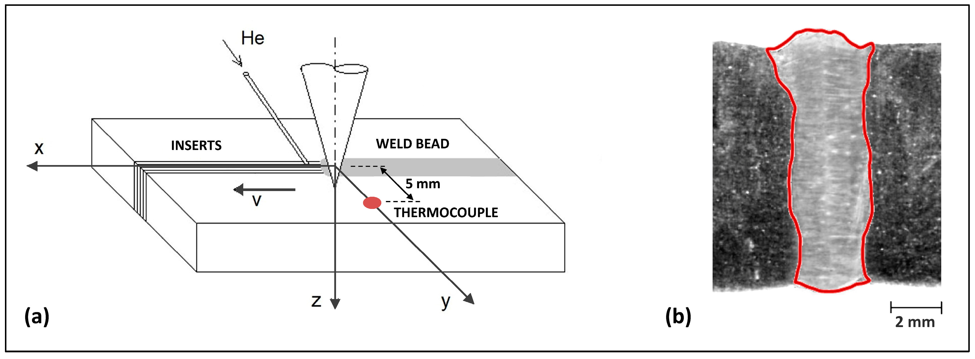
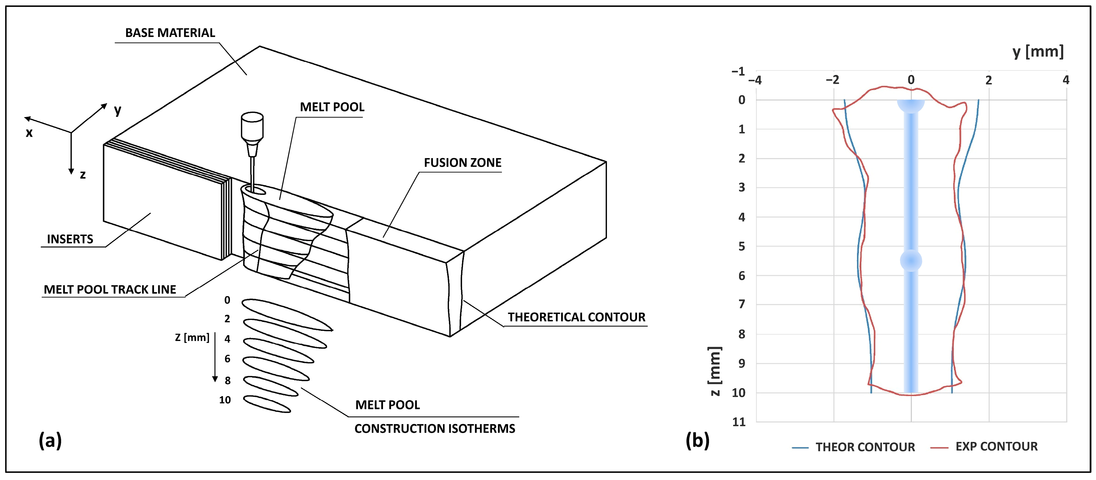


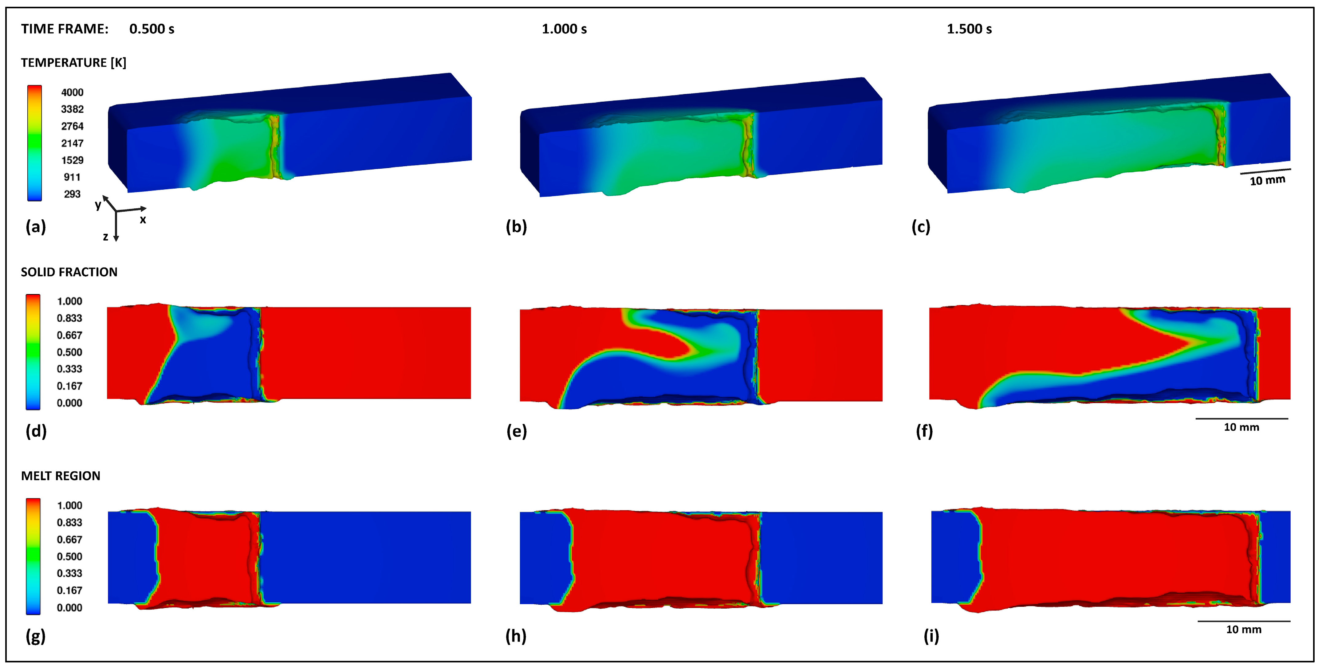


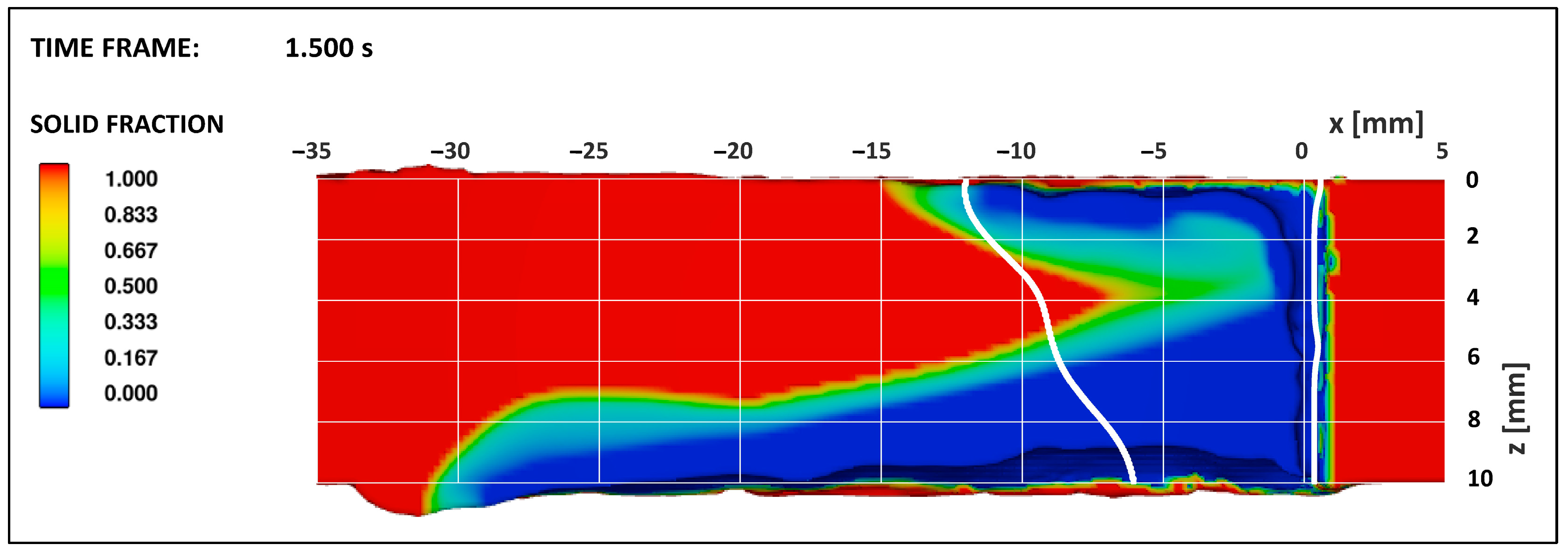
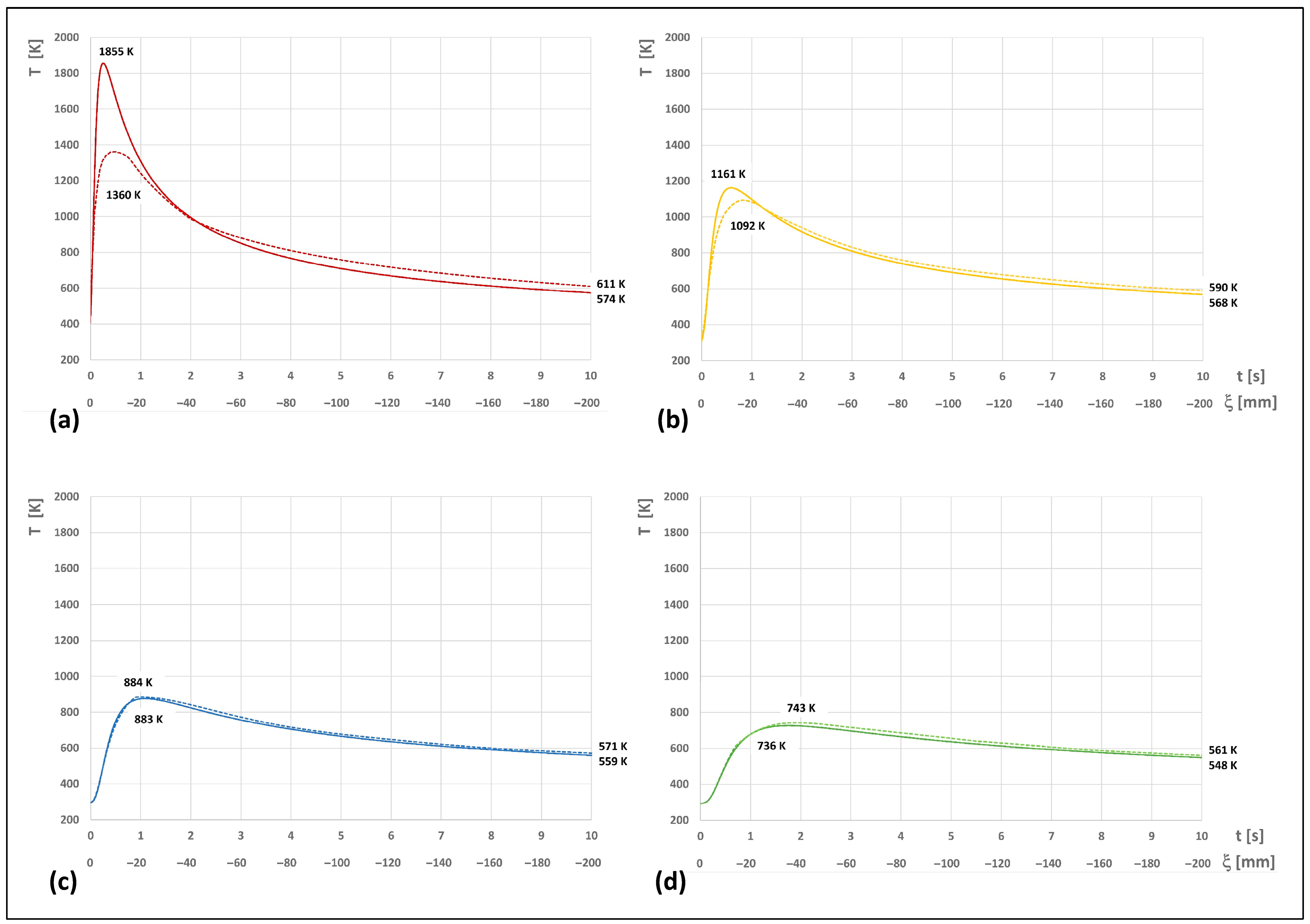
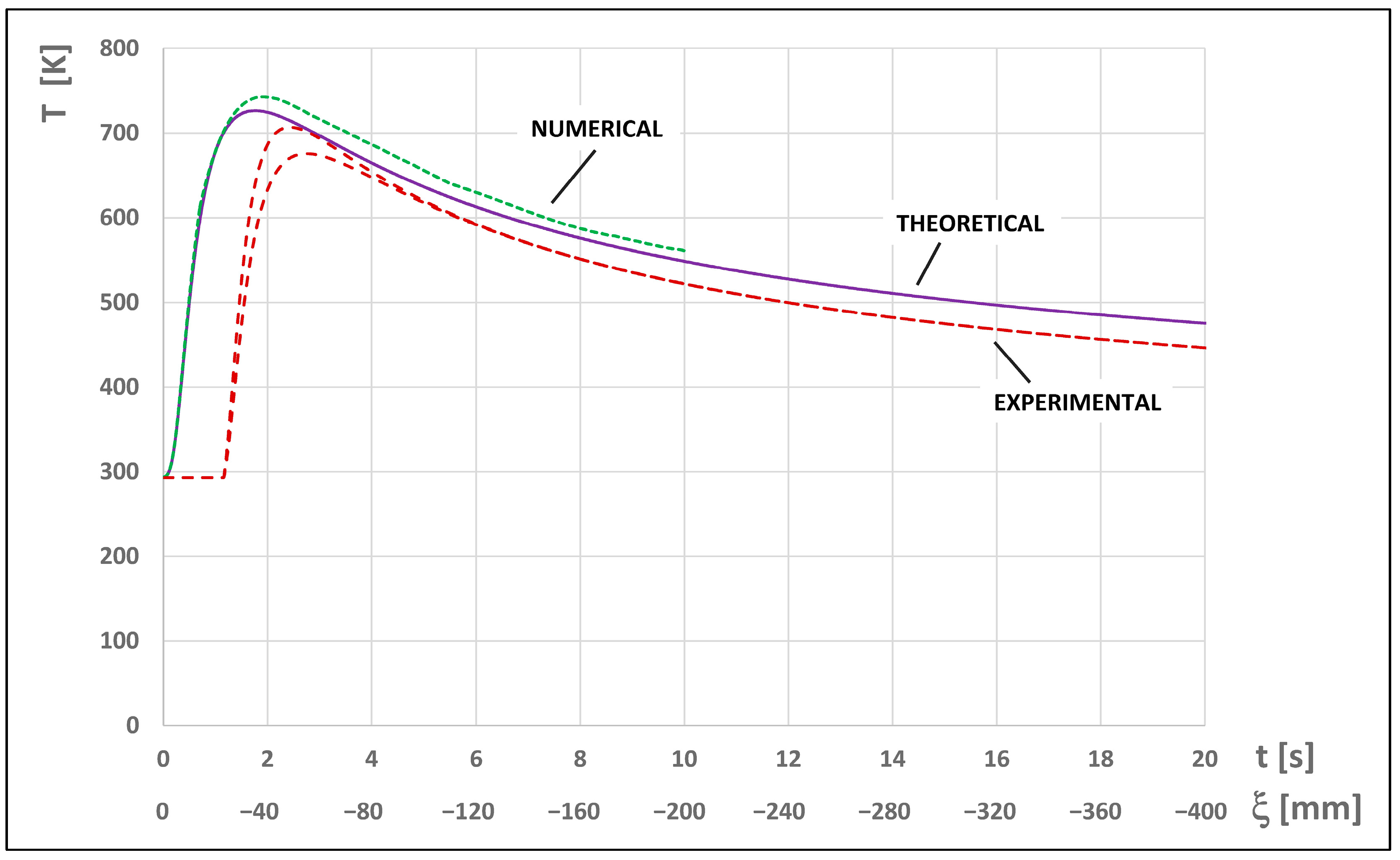
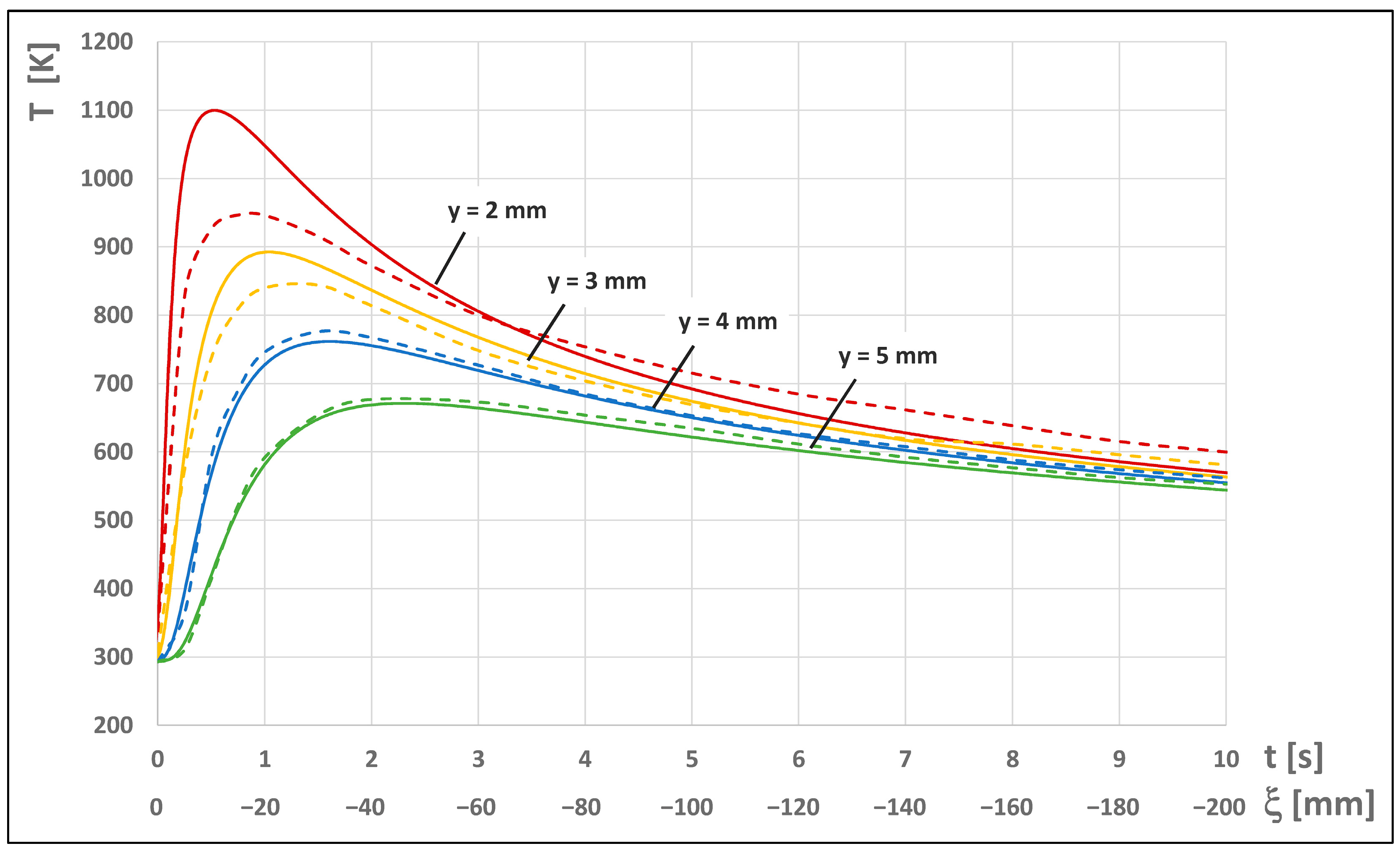
Disclaimer/Publisher’s Note: The statements, opinions and data contained in all publications are solely those of the individual author(s) and contributor(s) and not of MDPI and/or the editor(s). MDPI and/or the editor(s) disclaim responsibility for any injury to people or property resulting from any ideas, methods, instructions or products referred to in the content. |
© 2023 by the authors. Licensee MDPI, Basel, Switzerland. This article is an open access article distributed under the terms and conditions of the Creative Commons Attribution (CC BY) license (https://creativecommons.org/licenses/by/4.0/).