

Experimental Investigation and Modeling: Considerations of Simultaneous Surface Steel Droplets’ Evaporation and Corrosion
 ,
, 
 ,
, 
Abstract
:1. Introduction
2. Materials and Methods
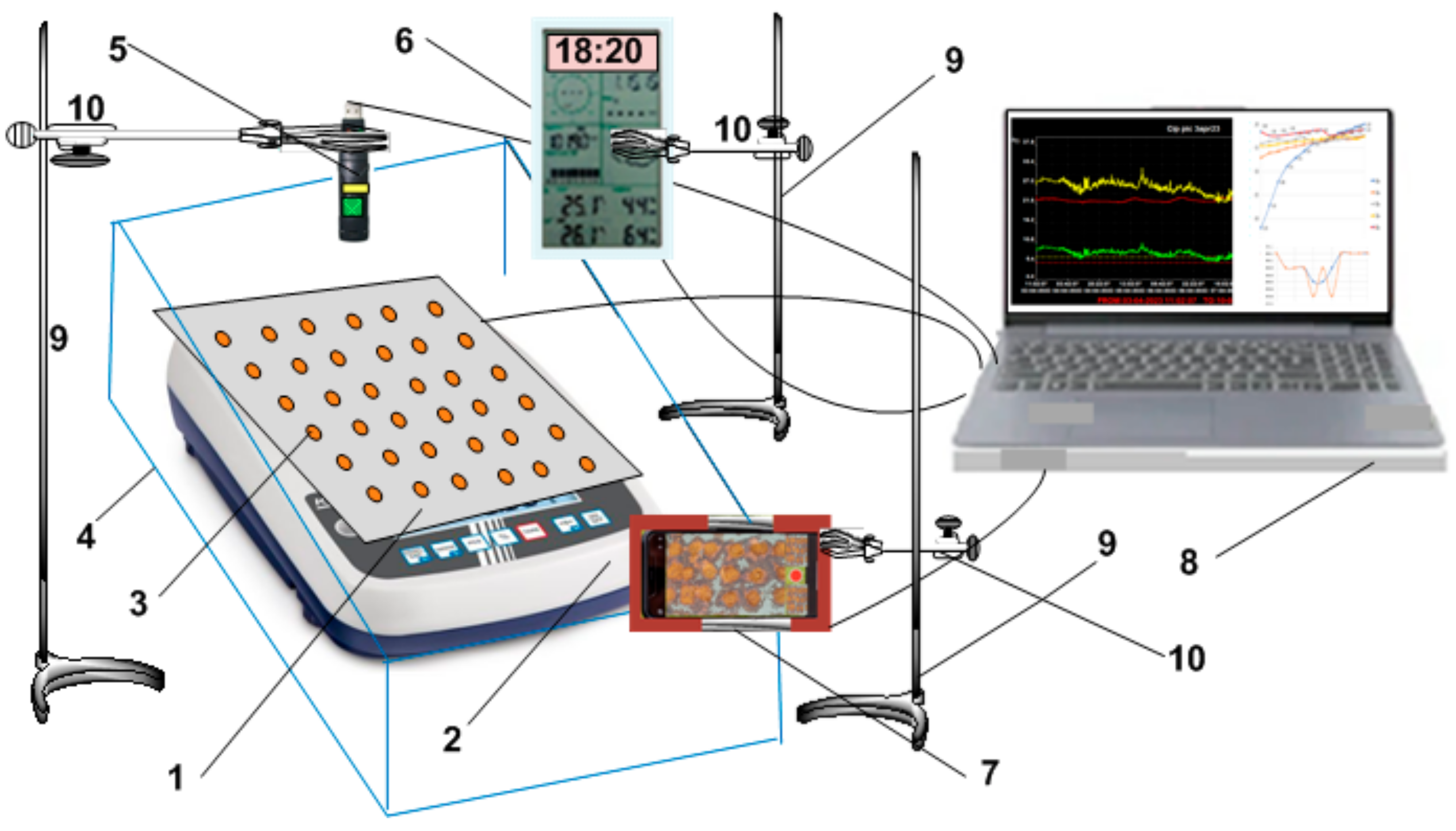
2.1. Experimental Setup and Procedures
- Determining the mass of the steel plate;
- Loading the plate with droplets in the preset positions;
- Starting the recording the momentary mass of the plate with droplets and the state of the moist air parameters near the surface (at ~8 cm from it);
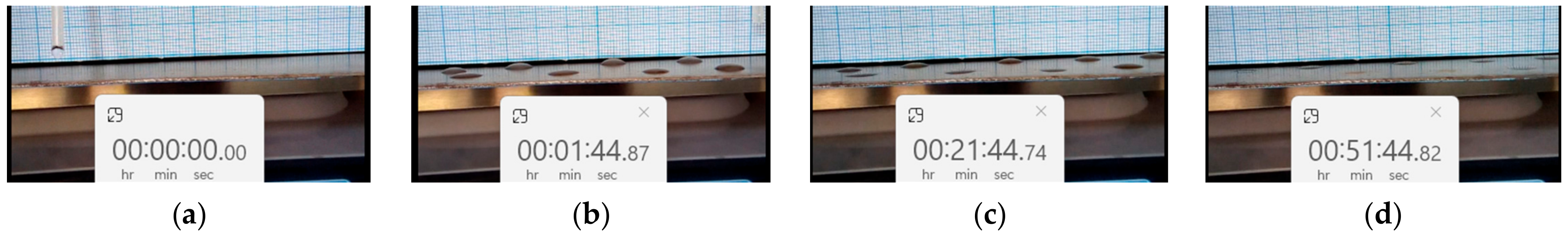
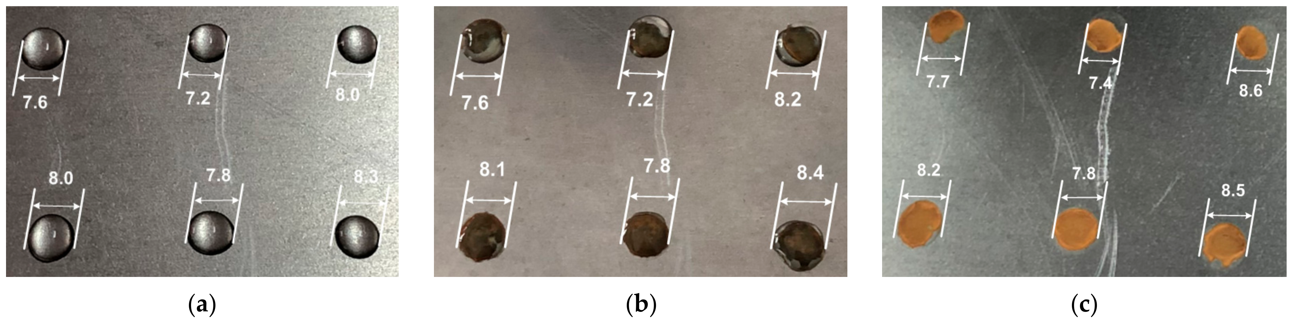
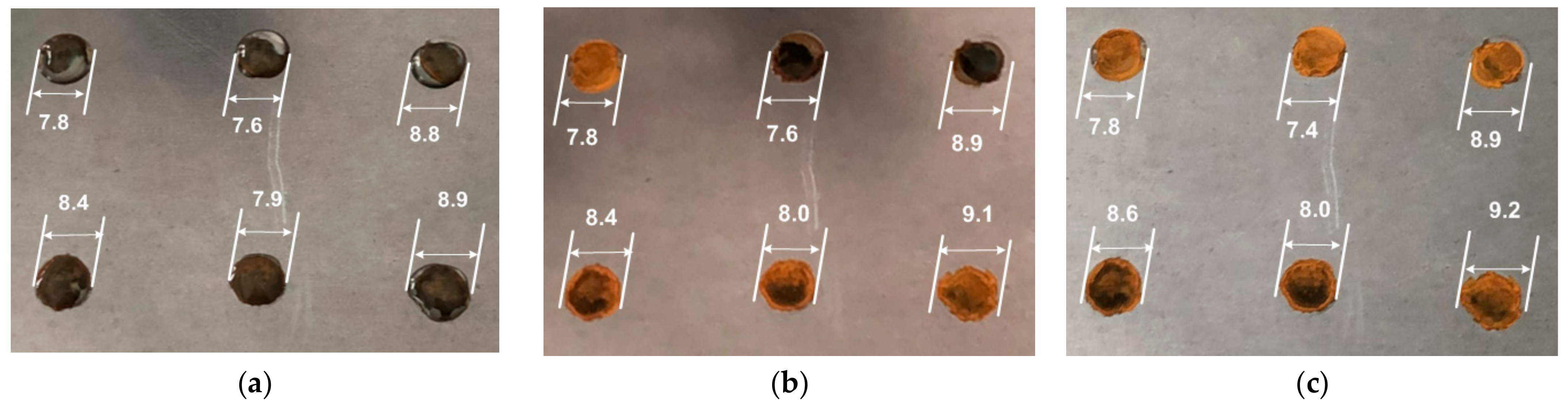
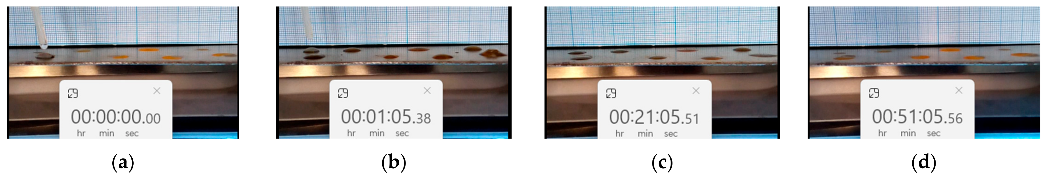
- Taking digital photographs of the plate with droplets at test starting, during the test and at the end of each test experiment;
- Ascertaining the drying of the droplets and saving the recordings in order to process them.
2.2. Mathematical Modeling
3. Results
- The water mass dynamics of the drops from the plate;
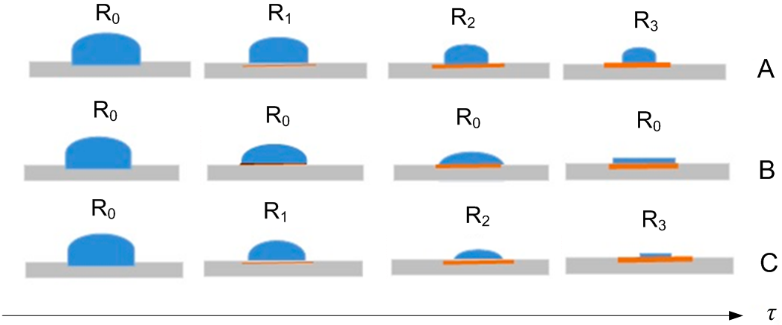
- The state of the evaporating drops’ shape;
- The air parameters near to the plate with the evaporating drops;
- The increase in plate mass due to rust deposition from corrosion process.
4. Discussion
- Completing the model with additional data (temperature dependence of dissolved oxygen concentration in water droplet, temperature dependence of water surface tension, densities, molecular masses, etc.) and conditions’ initials;
- The numerical transposition of the model with the micro sequences: (a) the choice of the parameters of the model that require calibration, namely the coefficient α and the power m in relation (21), the coefficient a in Equation (24), krs and the relation DO2efin (Equation (25)), respectively; (b) selection, from the beginning of the investigation, of the tests with all their data, which are used in the calibration (Table 5 and Table 6 for corrosion in water droplets, respectively, and Table 8 for corrosion with droplets containing NaCl); (c) setting an option regarding air parameters’ (relative humidity and temperature according to Table 5, Table 6, Table 7 and Table 8) use in the model, i.e., as functions of time or as average values; (d) the effective expression of the numerical model from the import of the test data file to the Runge–Kutta integration of the differential equations that provides the dynamics of the mass of the droplet and the dynamics of the mass of rust deposited under the droplet, respectively;
- The effective use of the numerical model in order to establish values for certain parameters, and strategies for expressing others, respectively.
5. Conclusions
Author Contributions
Funding
Institutional Review Board Statement
Informed Consent Statement
Data Availability Statement
Conflicts of Interest
References
- Gerhardus, K.H.; Michel, B.H.P.; Neil, T.G.; Virmani, P.Y.; Payer, J.H. Corrosion Costs and Preventives Strategies in the United States. Available online: https://impact.nace.org/documents/ccsupp.pdf (accessed on 3 August 2023).
- Ke, W.; Li, Z. Survey of Corrosion Cost in China and Preventive Strategies. Corros. Sci. Technol. 2008, 7, 259–264. [Google Scholar]
- Chico, B.; Fuente, D.; Díaz, J.; Simancas, J.; Morcillo, M. Annual Atmospheric Corrosion of Carbon Steel Worldwide. An Integration of ISOCORRAG, ICP/UNECE and MICAT Databases. Materials 2017, 10, 601. [Google Scholar] [CrossRef] [PubMed]
- Hou, W.; Liang, C. Atmospheric corrosion prediction of steels. Corrosion 2004, 60, 313–322. [Google Scholar] [CrossRef]
- Díaz, I.; Cano, H.; Chico, B.; De la Fuente, D.; Morcillo, M. Some clarifications regarding literature on atmospheric corrosion of weathering steels. Int. J. Corros. 2012, 2012, 812192. [Google Scholar] [CrossRef]
- Forolius, A.Z. The Kinetics of Anodic Dissolution of Iron in High Purity Water. Corros. Eng. 1979, 28, 10–17. [Google Scholar] [CrossRef] [PubMed]
- Klinesmith, D.E.; McCuen, R.; Albrecht, H.P. Effect of environmental conditions on corrosion rates. J. Mater. Civil. Eng. 2007, 19, 121–129. [Google Scholar] [CrossRef]
- Morcillo, M.; Chico, B.; Díaz, I.; Cano, H.; De la Fuente, D. Atmospheric corrosion data of weathering steels. A review. Corros. Sci. 2013, 77, 6–24. [Google Scholar] [CrossRef]
- To, D. Evaluation of Atmospheric Corrosion in Steels for Corrosion Mapping in Asia, Chapter 2. Ph.D. Thesis, Graduate School of Engineering, Yokohama National University, Yokohama, Japan, 2017. [Google Scholar]
- Ilie, M.C.; Maior, I.; Raducanu, C.E.; Deleanu, I.M.; Dobre, T.; Parvulescu, O.C. Experimental Investigation and Modeling of Film Flow Corrosion. Metals 2023, 13, 1425. [Google Scholar] [CrossRef]
- Tsuru, T.; Tamiya, K.I.; Nishikata, A. Formation and growth of microdroplets during the initial stage of atmospheric corrosion. Electrochim. Acta 2004, 49, 2709–2715. [Google Scholar] [CrossRef]
- Sainz-Rosales, A.; Ocampo-Lazcarro, X.; Hernández-Pérez, A.; González-Gutiérrez, A.G.; Larios-Durán, R.E.; Ponce de León, C.; Walsh, C.F.; Bárcena-Soto, M.; Casillas, N. Classic Evans’s Drop Corrosion Experiment Investigated in Terms of a Tertiary Current and Potential Distribution. Corros. Mater. Degrad. 2022, 3, 270–280. [Google Scholar] [CrossRef]
- Narhe, R.D.; González-Vinas, W.; Beysens, D.A. Water condensation on zinc surfaces treated by chemical bath deposition. Appl. Surf. Sci. 2010, 256, 4930–4933. [Google Scholar] [CrossRef]
- Lawrence, G.M. The relationship between relative humidity and the dewpoint temperature in moist air: A simple conversion and applications. Bull. Am. Meteorol. Soc. 2005, 86, 225–233. [Google Scholar] [CrossRef]
- Evans, U.R. Mechanism of rusting. Corros. Sci. 1969, 9, 813–821. [Google Scholar] [CrossRef]
- Chen, C.; Mansfeld, F. Potential distribution in the Evans drop experiment. Corros. Sci. 1997, 39, 409–413. [Google Scholar] [CrossRef]
- Venkatraman, M.S.; Cole, I.S.; Gunasegaram, D.R.; Emmanuel, B. Modelling Corrosion of a Metal under an Aerosol Droplet. Mater. Sci. Forum 2010, 654–656, 1650–1653. [Google Scholar] [CrossRef]
- Tejaswi, J.; Wang, Z.; Askounis, A.; Orejon, D.; Harish, S.; Takata, Y.; Mahapatra, P.S.; Pattamatta, A. Evaporation kinetics of pure water drops: Thermal patterns, Marangoni flow, and interfacial temperature difference. Phys. Rev. E 2018, 98, 052804. [Google Scholar]
- Hua, H.; Larson, R.G. Marangoni Effect Reverses Coffee-Ring Depositions. J. Phys. Chem. B 2006, 110, 7090–7096. [Google Scholar] [CrossRef]
- Yuri, O.P. Evaporative deposition patterns: Spatial dimensions of the deposit. Phys. Rev. E 2005, 71, 036313. [Google Scholar]
- Somlyai-Sipos, L.; Baumli, P. Wettability of Metals by Water. Metals 2022, 12, 1274. [Google Scholar] [CrossRef]
- Xu, J.; Li, B.; Lian, J.; Ni, J.; Xiao, J. Wetting behaviors of water droplet on rough metal substrates. Adv. Eng. Res. 2016, 9, 341–345. [Google Scholar]
- Dobre, T.; Pârvulescu, O.C.; Stoica-Guzun, A.; Stroescu, M.; Jipa, I.; Al Janabi, A.A. Heat and mass transfer in fixed bed drying of non-deformable porous particles. Int. J. Heat Mass Transf. 2016, 103, 478–485. [Google Scholar] [CrossRef]
- Dobre, T.; Zicman, L.R.; Pârvulescu, O.C.; Neacşu, E.; Ciobanu, C.; Drăgolici, F.N. Species removal from aqueous radioactive waste by deep-bed filtration. Environ. Pollut. 2018, 241, 303–310. [Google Scholar] [CrossRef] [PubMed]
- Duda, I.; Gradinaru, S. Calculation of areas in parametric coordinates. In Integral Calculus with Applications; Romania of Tomorrow Publishing House: Bucharest, Romania, 2007; pp. 394–452. ISBN 978-973-725-824-3. [Google Scholar]
- Xiongjiang, Y.; Jinliang, X. Does sunlight always accelerate water droplet evaporation? Appl. Phys. Lett. 2020, 116, 253903. [Google Scholar]
- Van Gaalen, R.T.; Diddens, C.; Wijshoff, H.M.A.; Kuerten, J.G.M. Marangoni circulation in evaporating droplets in the presence of soluble surfactants. J. Colloid Interface Sci. 2021, 584, 622–633. [Google Scholar] [CrossRef] [PubMed]
- Girard, F.; Antoni, M.; Sefiane, K. On the effect of Marangoni flow on evaporation rates of heated water drops. Langmuir 24. Am. Chem. Soc. 2008, 17, 9207–9210. [Google Scholar]
- Perry, H.D.; Green, W.D.; Malloney, O.J. Perry’s Chemical Engineering Handbook, 7th ed.; McGraw—Hill: San Francisco, CA, USA, 1997; pp. 78–80. [Google Scholar]
- Steeman, H.J.; Janssens, A.; De Paepe, M. On the applicability of the heat and mass transfer analogy in indoor air flows. Int. J. Heat Mass Transf. 2009, 52, 1431–1442. [Google Scholar] [CrossRef]
- Bird, B.R.; Stewart, E.W.; Lightftoot, N.E. Transport Phenomena, 2nd ed.; John Wiley & Sons: Hoboken, NJ, USA, 2002; pp. 442–443. [Google Scholar]
- Leca, A.; Pop, M.G.; Prisecaru, I.; Neaga, C.; Zidaru, G.H.; Musatescu, V.; Isbasoiu, E.C. Calculation Guide. Tables, Nomograms and Thermotechnical Formulas; Technical Publishing House: Bucharest, Romania, 1987; Volume 2, p. 71. [Google Scholar]
- Davies, J.T.; Rideal, E.K. Chapter: Mass Transfer across Interfaces. In Interfacial Phenomena; Academic Press: New York, NY, USA, 1963. [Google Scholar]
- Dobre, T.; Stoica, A. Mass Transfer Intensification; Electra Publishing House: Florence, Italy, 2017; Chapter 7. [Google Scholar]
- Ahmed, S.; Hou, Y.; Lepkova, K.; Pojtanabuntoeng, T. Investigation of the effect chloride ions on carbon steel in closed environments at different temperatures. Corros. Mater. Degrad. 2023, 4, 364–381. [Google Scholar] [CrossRef]
- Morcillo, M.; Chico, B.; Alcantara, J.; Diaz, I.; Simancas, J.; De la Fuente, D. Atmospheric corrosion of mild steel in chloride-rich environments. Questions to be answered. Mater. Corros. 2015, 66, 882–892. [Google Scholar] [CrossRef]


| Element | Composition (wt%) |
|---|---|
| Manganese (Mn) | 0.166 |
| Phosphorus (P) | 0.028 |
| Sulfur (S) | 0.028 |
| Carbon (C) | 0.206 |
| Chromium (Cr) | 0.078 |
| Molybdenum (Mo) | 0.114 |
| Vanadium (V) | 0.003 |
| Silicon (Si) | 0.004 |
| Copper (Cu) | 0.082 |
| Nickel (Ni) | 0.088 |
| Titanium (Ti) | 0.004 |
| Iron (Fe) | 0.199 |
| C.N. | Experimental Factors | Values | Observations |
|---|---|---|---|
| 1 | Number of drops on the plate | 100 | Selected |
| 2 | The initial mass of the drops on the plate (g) | 4.5–15.5 | Selected |
| 3 | Average droplet volume (μL) | 45–55 | Computed |
| 4 | The initial shape of the drop | Spherical cap | Observed |
| 5 | Electrical conductivity and water pH (μS/cm) | 100 | Selected |
| 6 | Number of successive tests for corrosion in water | 26 | Selected |
| 7 | NaCl concentration (g/L) in water (accelerated corrosion) | 1 | Selected |
| 8 | Number of accelerated corrosion tests | 4 | Selected |
| Parameters | Surface Values as Function of Droplet Mass | ||||||
|---|---|---|---|---|---|---|---|
| R (cm) | 0.30 | ||||||
| mp (g) | 0.060 | 0.050 | 0.040 | 0.030 | 0.020 | 0.010 | 0.005 |
| h or hτ (cm) | 0.312 | 0.276 | 0.235 | 0.183 | 0.133 | 0.069 | 0.035 |
| S or S(τ) (cm2) | 0.588 | 0.528 | 0.453 | 0.378 | 0.286 | 0.283 | 0.283 |
| ) | |||||||
| R (cm) | 0.35 | ||||||
| mp (g) | 0.060 | 0.050 | 0.040 | 0.030 | 0.020 | 0.010 | 0.005 |
| h or hτ (cm) | 0.252 | 0.228 | 0.189 | 0.147 | 0.101 | 0.052 | 0.022 |
| S or S(τ) (cm2) | 0.595 | 0.530 | 0.458 | 0.385 | 0.385 | 0.385 | 0.385 |
| ) | |||||||
| R (cm) | 0.40 | ||||||
| mp (g) | 0.060 | 0.050 | 0.040 | 0.030 | 0.020 | 0.010 | 0.005 |
| h or hτ (cm) | 0.217 | 0.185 | 0.152 | 0.116 | 0.078 | 0.040 | 0.020 |
| S or S(τ) (cm2) | 0.601 | 0.529 | 0.505 | 0.503 | 0.503 | 0.503 | 0.503 |
| ) | |||||||
| R (cm) | 0.45 | ||||||
| mp (g) | 0.060 | 0.050 | 0.040 | 0.030 | 0.020 | 0.010 | 0.005 |
| h or hτ (cm) | 0.179 | 0.157 | 0.123 | 0.093 | 0.062 | 0.031 | 0.016 |
| S or S(τ) (cm2) | 0.666 | 0.656 | 0.642 | 0.636 | 0.636 | 0.636 | 0.636 |
| ) | |||||||
| C.N. | Parameter | Vertical Surface | Horizontal Upper Surface | Horizontal Lower Surface |
|---|---|---|---|---|
| 1 | 1.420 | 1.320 | 1.520 | |
| 2 | 0.250 | 0.250 | 0.330 | |
| 3 | 0.112 | 0.055 | 0.055 |
| A | B | C | D | E | F | G | H | I | J | K | L | M |
|---|---|---|---|---|---|---|---|---|---|---|---|---|
| 1 | 0 | 482.15 | 487.25 | 0.00 | 0.05 | 27.7 | 53.9 | 17.5 | 26.0 | 55.0 | 757.6 | 0.0 |
| 2 | 30 | 486.35 | 0.90 | 27.8 | 52.9 | 17.3 | 0.5 | |||||
| 3 | 60 | 485.30 | 1.05 | 27.9 | 53.3 | 17.5 | 1.0 | |||||
| 4 | 90 | 484.00 | 1.30 | 27.9 | 52.8 | 17.3 | 1.5 | |||||
| 5 | 120 | 483.50 | 0.50 | 28.0 | 52.1 | 17.2 | 2.0 | |||||
| 6 | 150 | 482.80 | 0.70 | 27.8 | 52.8 | 17.2 | 2.5 | |||||
| 7 | 180 | 482.20 | 0.60 | 27.8 | 52.9 | 17.3 | 3.0 | |||||
| 8 | 210 | 482.20 | 0.00 | 27.8 | 53.2 | 17.3 | 3.5 |
| A | B | C | D | E | F | G | H | I | J | K | L | M |
|---|---|---|---|---|---|---|---|---|---|---|---|---|
| 1 | 0 | 482.30 | 486.85 | 0.00 | 0.05 | 27.2 | 43.2 | 13.6 | 2.0 | 44.0 | 756 | 81.0 |
| 2 | 30 | 484.35 | 2.50 | 27.4 | 42.8 | 13.6 | 81.5 | |||||
| 3 | 60 | 484.10 | 0.25 | 27.5 | 42.5 | 13.6 | 82.0 | |||||
| 4 | 90 | 482.80 | 1.30 | 27.7 | 41.9 | 13.5 | 82.5 | |||||
| 5 | 120 | 482.35 | 0.00 | 27.9 | 40.9 | 13.3 | 83.0 | |||||
| 6 | 150 | 482.35 | 0.00 | 27.8 | 40.9 | 13.3 | 83.5 |
| A | B | C | D | E | F | G | H | I | J | K | L | M |
|---|---|---|---|---|---|---|---|---|---|---|---|---|
| 1 | 0 | 484.45 | 501.60 | 0.00 | 0.25 | 28.5 | 32.2 | 10.3 | 32 | 45 | 759 | 9711.5 |
| 2 | 30 | 498.00 | 3.60 | 28.3 | 31.7 | 9.8 | 9712.0 | |||||
| 3 | 60 | 497.30 | 0.70 | 28.2 | 33.4 | 10.5 | 9712.5 | |||||
| 4 | 90 | 495.40 | 1.90 | 28.3 | 32.6 | 10.3 | 9713.0 | |||||
| 5 | 120 | 492.35 | 3.05 | 28.1 | 32.2 | 9.9 | 9713.5 | |||||
| 6 | 150 | 490.20 | 2.15 | 28.1 | 32.1 | 9.9 | 9714.0 | |||||
| 7 | 180 | 488.40 | 1.80 | 28.0 | 31.7 | 9.6 | 9714.5 | |||||
| 8 | 210 | 487.65 | 0.75 | 28.0 | 31.8 | 9.6 | 9715.0 | |||||
| 9 | 240 | 486.30 | 1.35 | 27.9 | 32.4 | 9.8 | 9715.5 | |||||
| 10 | 270 | 485.40 | 0.90 | 27.8 | 33.1 | 10.1 | 9716.0 | |||||
| 11 | 300 | 484.85 | 0.55 | 27.7 | 33.6 | 10.2 | 9716.5 | |||||
| 12 | 330 | 484.85 | 0.00 | 27.6 | 34.1 | 10.3 | 9717.0 |
| A | B | C | D | E | F | G | H | I | J | K | L | M |
|---|---|---|---|---|---|---|---|---|---|---|---|---|
| 1 | 0 | 485.20 | 496.15 | 0.00 | 0.30 | 28.9 | 37.8 | 13 | 30 | 35 | 757 | 9769.0 |
| 2 | 30 | 493.10 | 3.05 | 29.1 | 37.6 | 13.1 | 9769.5 | |||||
| 3 | 60 | 491.20 | 1.90 | 29.2 | 37.7 | 13.3 | 9770.0 | |||||
| 4 | 90 | 489.35 | 1.85 | 29.0 | 36.9 | 12.7 | 9770.5 | |||||
| 5 | 120 | 488.15 | 1.20 | 28.8 | 37.1 | 12.7 | 9771.0 | |||||
| 6 | 150 | 486.70 | 1.45 | 28.7 | 37.1 | 12.6 | 9771.5 | |||||
| 7 | 180 | 485.50 | 1.20 | 28.6 | 37.1 | 12.5 | 9772.0 | |||||
| 8 | 210 | 485.50 | 0.00 | 28.5 | 36.7 | 12.2 | 9772.5 |
| C.N. | Case | Data | φ | tg | (Equation (25)) | (Equation (23)) | a (Equation (21)) | m (Equation (21)) | α (Equation (24)) |
|---|---|---|---|---|---|---|---|---|---|
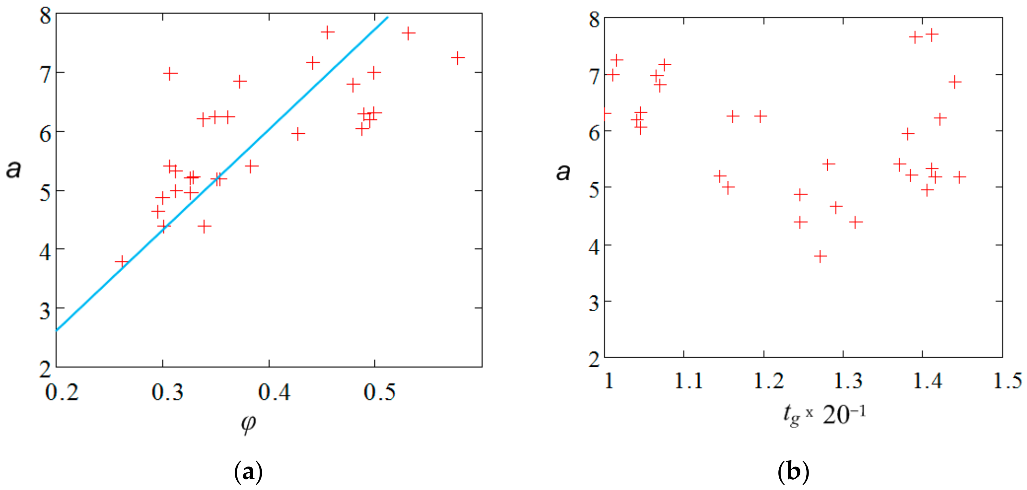
| 1 | Water droplet | Table 5 Table 6 | mean | mean | 4.5 × 10⁻⁵ (m/s) | 9.1 × 10⁻¹⁰ (m2/s) | f(φ,tg) | 0.33 | 2.63 × 10⁻⁴ (m2·s) |
| 2 | Water droplet with NaCl | Table 8 | mean | mean | 9.5 × 10⁻⁴ (m/s) | 5.1 × 10⁻⁹ (m2/s) | f(φ,tg) | 0.33 | 2.63 × 10⁻⁴ (m2·s) |
| Test | mp0 (g) | φ (/) | tg (°C) | a (20) | εmpM (%) | εmruM (%) | τt (h) | τc (h) | τp (h) |
|---|---|---|---|---|---|---|---|---|---|
| 1 | 0.0500 | 0.531 | 27.8 | 7.66 | −8.14 | −9.31 | 3.5 | 3.5 | 3.5 |
| 2 | 0.0480 | 0.454 | 28.2 | 7.69 | −7.65 | −2.85 | 3.0 | 6.5 | 30.5 |
| 3 | 0.0360 | 0.354 | 28.3 | 5.18 | 11.31 | 2.94 | 2.5 | 9.0 | 57.5 |
| 4 | 0.0455 | 0.427 | 27.6 | 5.95 | 18.62 | 1.94 | 2.5 | 11.5 | 83.5 |
| 5 | 0.0490 | 0.328 | 27.7 | 5.23 | 15.18 | 4.39 | 3.0 | 14.5 | 134 |
| 6 | 0.0480 | 0.306 | 27.4 | 5.41 | −11.50 | 15.55 | 2.5 | 17.0 | 161 |
| 7 | 0.0535 | 0.312 | 28.2 | 5.33 | 14.14 | 8.65 | 2.5 | 19.5 | 187 |
| 8 | 0.0535 | 0.350 | 28.9 | 5.19 | 0.717 | 11.02 | 3.0 | 22.5 | 214 |
| 9 | 0.0630 | 0.383 | 25.6 | 5.41 | 15.29 | 5.62 | 4.0 | 26.5 | 1658 |
| 10 | 0.0700 | 0.339 | 26.3 | 4.39 | 1.81 | −161 | 4.5 | 31.0 | 1687 |
| 11 | 0.0915 | 0.479 | 21.4 | 6.80 | 8.45 | 2.35 | 5.0 | 36.0 | 2892 |
| 12 | 0.1040 | 0.441 | 21,5 | 7.16 | −12.74 | 3.83 | 4.0 | 40.0 | 2920 |
| 13 | 0.1020 | 0.301 | 24.9 | 4.39 | 18.00 | 4.79 | 5.0 | 45.0 | 5517 |
| 14 | 0.1150 | 0.261 | 25.4 | 3.79 | −0.96 | 2.45 | 5.0 | 50.0 | 5645 |
| 15 | 0.1230 | 0.950 | 25.8 | 4.65 | −13.42 | 4.68 | 5.0 | 55.0 | 5575 |
| 16 | 0.1310 | 0.299 | 24.9 | 4.88 | −1.39 | 2.92 | 5.0 | 60.0 | 6252 |
| 17 | 0.1320 | 0.349 | 23.9 | 6.26 | −3.21 | 4.86 | 5.0 | 64.0 | 6282 |
| 18 | 0.1240 | 0.361 | 23.2 | 6.25 | −3.49 | 7.19 | 5.5 | 69.5 | 6584 |
| 19 | 0.1260 | 0.306 | 21.3 | 6.97 | −3.31 | 7.96 | 5.0 | 74.5 | 6603 |
| 20 | 0.1350 | 0.326 | 22.9 | 5.21 | −4.41 | 8.72 | 6.0 | 80.5 | 6663 |
| 21 | 0.1460 | 0.312 | 23.1 | 5.01 | 0.48 | 9.66 | 5.5 | 86.0 | 6903 |
| 22 | 0.1670 | 0.498 | 20.9 | 5.31 | 1.75 | 9.92 | 7.5 | 93.5 | 7014 |
| 23 | 0.1390 | 0.498 | 20.2 | 6.99 | 3.04 | 9.71 | 7.0 | 100.5 | 7654 |
| 24 | 0.1500 | 0.489 | 20,0 | 6.30 | −6.20 | 11.24 | 7.5 | 108.0 | 7684 |
| 25 | 0.1670 | 0.487 | 20.9 | 6.05 | 16.75 | 12.89 | 8.5 | 116.5 | 7719 |
| 26 | 0.1650 | 0.577 | 20,3 | 7.26 | 5.16 | 11.08 | 8.5 | 125.0 | 7789 |
| 27 | 0.2080 | 0.495 | 20.8 | 5.19 | 17.87 | 8.95 | 9.5 | 134.5 | 7820 |
| 28 | 0.1250 | 0.326 | 28.1 | 5.95 | 15.18 | 12.27 | 5.5 | 140.0 | 7860 |
| 29 | 0.1550 | 0.337 | 28.4 | 6.21 | 15.28 | 13.27 | 4.0 | 144.0 | 7884 |
| 30 | 0.1090 | 0.372 | 28.8 | 6.86 | −19.98 | 17.31 | 3.5 | 147.5 | 7908 |
Disclaimer/Publisher’s Note: The statements, opinions and data contained in all publications are solely those of the individual author(s) and contributor(s) and not of MDPI and/or the editor(s). MDPI and/or the editor(s) disclaim responsibility for any injury to people or property resulting from any ideas, methods, instructions or products referred to in the content. |
© 2023 by the authors. Licensee MDPI, Basel, Switzerland. This article is an open access article distributed under the terms and conditions of the Creative Commons Attribution (CC BY) license (https://creativecommons.org/licenses/by/4.0/).
Share and Cite
Ilie, M.C.; Chiş, T.V.; Maior, I.; Răducanu, C.E.; Deleanu, I.M.; Dobre, T.; Pârvulescu, O.C. Experimental Investigation and Modeling: Considerations of Simultaneous Surface Steel Droplets’ Evaporation and Corrosion. Metals 2023, 13, 1733. https://doi.org/10.3390/met13101733
Ilie MC, Chiş TV, Maior I, Răducanu CE, Deleanu IM, Dobre T, Pârvulescu OC. Experimental Investigation and Modeling: Considerations of Simultaneous Surface Steel Droplets’ Evaporation and Corrosion. Metals. 2023; 13(10):1733. https://doi.org/10.3390/met13101733
Chicago/Turabian StyleIlie, Marius Ciprian, Timur Vasile Chiş, Ioana Maior, Cristian Eugen Răducanu, Iuliana Mihaela Deleanu, Tănase Dobre, and Oana Cristina Pârvulescu. 2023. "Experimental Investigation and Modeling: Considerations of Simultaneous Surface Steel Droplets’ Evaporation and Corrosion" Metals 13, no. 10: 1733. https://doi.org/10.3390/met13101733
APA StyleIlie, M. C., Chiş, T. V., Maior, I., Răducanu, C. E., Deleanu, I. M., Dobre, T., & Pârvulescu, O. C. (2023). Experimental Investigation and Modeling: Considerations of Simultaneous Surface Steel Droplets’ Evaporation and Corrosion. Metals, 13(10), 1733. https://doi.org/10.3390/met13101733