Corrosion Behavior of Copper Exposed in Marine Tropical Atmosphere in Rapa Nui (Easter Island) Chile 20 Years after MICAT

Abstract

Atmospheric corrosion of copper, exposed on a tropical island in the South-Central Pacific Ocean, was reported and compared with those of a very similar study at the same site conducted 20 years earlier. The new measurements—taken over three years of exposure, from 2010 to 2013—quantified corrosion by mass loss, characterized corrosion products by X-ray diffraction (DRX) and Raman techniques, observed the attack morphology by Scanning Electron Microscope (SEM), and evaluated the patina resistance using electrochemical techniques. The results showed a copper corrosivity category of C4, and the main copper patina compound, cuprite, was porous, nonhomogeneous, and thin. Electrochemical measurements showed cuprite layer growth as a function of the exposure time, and the morphology did not favor corrosion protection. Finally, when comparing the results to those of a study 22 years previous, the copper corrosion rates increased only slightly, even with increased contaminants associated with growing local populations and continuous tourism on the island.

1. Introduction

Atmospheric corrosion, a worldwide concern, is largely responsible for degrading the useful life of exposed metals, structures, and materials across rural, urban, industrial, marine, and marine–industrial environments [1,2,3,4,5,6,7]. In 1988, the Ibero-American Map of Atmospheric Corrosiveness (MICAT, Mapa Iberoamericano de Corrosión Atmosférica) project—which set out to evaluate the behavior of carbon steel, copper, zinc, and aluminum across multiple sites—further confirmed the influence of atmospheric and meteorochemical variables on corrosion [4,5,8]. Indeed, a useful structural life is determined by variables such as relative humidity; temperature; precipitation; wind speed and direction; and atmospheric pollution (environmental chloride, sulfur dioxide, and nitrogen oxides, among others) [9,10]. Studies have additionally found an explanatory variance in the angle of exposure and the height above sea level [11,12].

Carried out 20 years after the MICAT project cited above—which created local atmospheric corrosion maps in Chile [13,14,15], this article provides a much-needed update on copper corrosion behavior in Rapa Nui (Easter Island) and compares it with previous results (1988–1994). This site comparison focuses on Rapa Nui, an island located in the middle of the South Pacific Ocean with practically nonexistent industrial development; however, populations—as well as the number of tourists visiting the island—have grown considerably in recent decades. Given increased ENSO intensities and climate change, this isolated ocean site is ideal for the study of atmospheric corrosion phenomena [15,16,17].

The Rapa Nui Island climate is considered tropical temperate [17]. Previous authors have investigated the atmospheric corrosion of some materials in coastal and coastal-tropical environments. Castañeda et al. [18] evaluated carbon steel, galvanized steel, copper, and aluminum at sites of differing meteorochemical conditions across Cuba, demonstrating that variations in relative humidity and temperature significantly influence the deposition of environmental chloride and that reduced water movement in winter decreases coastal water salinity, therefore lowering corrosion rates. Depending on the study conditions near coastal edges, corrosion aggressiveness has been found to be CX and >CX for carbon steel and copper and aluminum at, and for, galvanized steel, C4 [1,2,18,19,20]. In a subtropical study, copper exposed in the Canary Islands archipelago has a ranked corrosivity category higher than CX [21] and C5 in Taking Taichung Harbor [22].

Additionally, Vera et al. found that the behavior of copper and patina color in coastal areas depend on chloride content, temperature, and relative humidity, as well as rainfall [23]. Other authors have shown that, as a function of exposure time, the atmospheric corrosion of copper in areas with salinity levels between 110 mg m⁻² d⁻¹ and 1640 mg m⁻² d⁻¹ forms superficial copper chlorides (Cu₂(OH)₃Cl), such as atacamite and clinoatacamite, and cuprite (Cu₂O) in the inner layers. The coating and sealing of cuprite by basic chlorides occurs mainly in areas where moisture is retained for a longer time and salinity is higher as a result of evaporation of the aqueous phase during the drying period [24].

Generally, copper patinas are chemically and structurally complex and have inhomogeneous surfaces, degrees of porosity, and sometimes loss of adhesion, making them prone to retaining moisture and atmospheric pollutants [25,26,27,28]. Copper patinas formed centuries ago show variable uniformity and behavior against atmospheric corrosion [27,29]. The ingress of chloride ions through patina defects can cause a localized attack on the underlying copper [26].

Pan et al. [30], while reporting on copper in a simulated coastal–industrial atmosphere, with corrosion as a function of the exposure time, reported that the main corrosion products formed were Cu₂O, Cu₂Cl(OH)₃, and Cu₄Cl₂(OH)₆, and, in the presence of SO₂, mainly Cu₄Cl₂(OH)₆. Additionally, Mendoza et al. identified cuprite, paratacamite, posnjakite, and brochantite as copper corrosion products in the tropical climate of Cuba [31].

The present work is thus nestled in the tradition of Atmospheric Corrosion Maps in Chile and in Latin America, as well as those under similar environmental conditions, seeking to report atmospheric corrosion behaviors of copper on Rapa Nui from 2010 to 2013 and to compare them against the results obtained from 1988 to 1994.

2. Materials and Methods

2.1. Place, Sample Preparation, Installation, and Meteorological Measurements

Rapa Nui (also known as Easter Island) is subtropical, with narrow seasonal temperature variations as mediated by oceanic temperance. The annual average is 21 °C, with a gentle seasonal range of 5 °C on average between 18 °C in the Austral winter (July–September) and 23–24 °C in the Austral summer (January–March). The total annual rainfall ranges between 1100 and 1300 mm, with an average of 140 rainy days. The average seasonal variability ranges between the minima of 70–80 mm/month (November to December) and maxima of 100–130 mm/month (April–June). The seasonal variability in precipitation results from the interplay of three climate systems: the South Pacific Anticyclone (SPA), the South Pacific Convergence Zone (SPCZ), and the westerly storm tracks (Figure 1).

Concerning the study, a frame containing 99.9% pure copper samples (Figure 2A) was installed at the assay site located within the Chilean Navy Base (Lat. 27.1565, Long. 109.4383; 22 m.a.s.l; 500 m from the coastline). Standard copper specimens (10 cm × 10 cm × 0.4 cm) were all exposed at an angle of 45° and separated by plastic insulators, following ISO 9223–9226 [32,33,34,35]. Prior to atmospheric exposure, the specimens were degreased with acetone, washed with high-purity water, dried with cold air, and stored in a desiccator. The cleaned and dried specimens were accurately measured and massed, ASTM G1–03 [36].

Meteorological parameters recorded at each test station included the mean annual temperature (T) (°C), mean annual relative humidity (RH) (%), rainfall (mm), wind speed (m/s), and time of wetness (TOW), calculated as the number of hours for which RH ≥ 80% and T > 0 °C and expressed in hours per year. The deposition rates of atmospheric SO₂ (mg SO₂ m⁻² d⁻¹) and Cl^– (mg Cl⁻ m⁻² d⁻¹) were also calculated in accordance with ISO 9223 [32] (Figure 2B,C).

The study period was from April 2010 to April 2013 (3 years of sample exposure). Specimens were installed in the month of April, corresponding to autumn in the Southern Hemisphere.

2.2. Corrosion Testing

The deterioration of the material was evaluated every 3 months by measuring the mass loss in triplicate (ASTM G50) [37]. The morphology of the attack was observed under a scanning electron microscope (SEM) using a Hitachi SU 3500 with a 410-M EDAX analyzer for elemental characterization.

Corrosion products were identified using a BRUKER DRX (model D8 Advance, Karlsruhe, Germany), with Cu-Kα radiation, and a 40 KV/30 mA graphite monochromator with a scanning range of 10–70°. The corrosion products were also analyzed using Raman spectra, recorded using a Renishaw Invia Raman spectrophotometer (Great Britain) equipped with a 532-nm laser excitation source and a thermally cooled CCD camera as the detector. The resolution was set to 4 cm⁻¹, with 10 scans at an integration time of 10-s recording spectra in the region of 100–4000 cm⁻¹ using a 50 $\times$ objective. The laser power was adjusted to 1%.

Infrared spectra (FT-IR) were recorded in a JASCO FT-IR 4600 infrared spectrophotometer (Tokyo, Japan) equipped with a DLaTGS detector. The spectral resolution in all cases was 4 cm⁻¹ with 32 accumulations per spectrum. The spectral range was 4000–400 cm⁻¹. The infrared spectra were obtained by potassium bromide (KBr) scattering.

A glow discharge optical emission spectroscopy (GDOES) depth profile analysis of the corrosion products was additionally obtained using a Spectruma Analytik GmbH GDA 750 HR (Hof, Germany) equipped with a 2.5-mm diameter anode and operating in DC excitation mode (constant voltage–constant current mode). Every sample was measured in duplicate. A glow was obtained under an argon atmosphere (5.0 quality) with an average discharge pressure of 5 × 10⁻² hPa. The excitation parameters were set to 1000 V and 12 mA, with the sputtering rate being calculated so that the measuring depth was at least 10 µm.

Finally, the protective character of the corrosion products formed on the materials was studied by, first, anodic polarization curves in 0.1 M Na₂SO₄ solution at 25 °C in aerated conditions with a sweep rate of 0.5 mV s⁻¹ using an Autolab potentiostat model 302 A, with a saturated calomel reference electrode and a platinum wire counter electrode, and second, electrochemical impedance spectroscopy measurements in an Autolab galvanostat Gamry cell with three electrodes, with copper specimen working electrodes with an exposed surface area of approximately 15 cm² in 0.1 M Na₂SO₄ electrolyte in aerated conditions and a high-purity (99.99%) platinum counter electrode and a saturated calomel electrode as the reference electrode. In both cases, the open circuit potential (OCP) was recorded until a steady state was reached, and impedance plots were obtained in a frequency range from 100 kHz to 10 mHz, with eight points per decade and using a sinusoidal amplitude of 10 mV peak-to-peak at E = OCP.

3. Results and Discussion

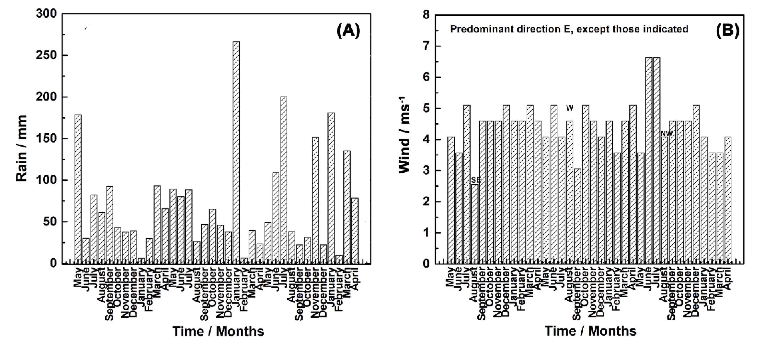
3.1. Characterization of the Test Atmosphere

Typical of oceanic islands at intermediate latitudes, the island has a tropical rainy climate (Af) that combines mild temperatures year-round, with very mild winters lacking frost or extreme cold. Its thermal regime shows an oceanic influence, with narrow daily and annual thermal oscillation. Rainfall, on the other hand, is distributed regularly throughout the year, reaching an average of 1000 mm per year. This is of convective origin, particularly in the summer season; however, during winter, the presence of some low-pressure systems brings rainfall from cold fronts. Köppen confirmed this by placing the island as having a tropical temperate with an average annual temperature of 20.5 °C between its maximum 29.7 °C in February and its minimum of 10.8 °C during August. The average relative humidity does not exceed 75%, and sunny days are around 30% of the year. The salinity of the seawater fluctuates between 35.0 and 36.4 PSU, whose variation depends on the season and the depth at which the sample is taken. As an example, the average salinity at a 4-m depth in 1999 was 35.88 PSU (T° 20.8 °C) and, at the same depth in 2015, was 35.60 PSU (T° 19.8 °C) [38].

Within this study, meteorological variables—relative humidity, temperature, wind speed, and precipitation—were recorded daily and compiled monthly. The relative humidity and temperature data together estimated the time of wetting (TOW) [39]. Figure 3 shows variations in the temperature, relative humidity, and wetting time during the three years of study, obtaining an average temperature of 20.6 °C (similar to that reported in the MICAT project), an average minimum temperature of 14.1 °C, and an average maximum temperature of 25.6 °C. The warmest months were between December and May, the least warm being between June and October. The average relative humidity was 72.7% (slightly lower than the value obtained in the MICAT project of 79.0%), with the average minimum RH 54.4% and average maximum 88.2%. With respect to the wetting time, the average throughout the 3 years of exposure was 3344 h/year, classified according to ISO 9223 [32] in τ4. However, some daily ambient temperatures may have seen sharp increases, causing evaporation of the electrolyte and, consequently, resulted in a decreased wetting time. According to the average value calculated for TOW, the metal surface was covered by water film for about 38% of the time in relation to the total number of hours per year (8760 h/year). The exact value of the TOW reached in the MICAT project for the area under study is not available. However, the average values of the temperature and relative humidity are similar to those obtained in the present study; therefore, a τ4 classification can be estimated.

Figure 4 shows the variation of ambient chloride (Figure 4A) and sulfur dioxide (Figure 4B) contents during the study period. The first year of exposure reached an average of 53.04 mg m⁻²d⁻¹ for the chloride content; the second year, an average of 51.13 mg m⁻² d⁻¹; and the third year, an average of 48.37 mg m⁻² d⁻¹. All these values correspond to an S1 classification, according to ISO 9223. On the other hand, the average environmental content of sulfur dioxide for the first year was 1.89 mg m⁻² d⁻¹ (classification P0, rural atmosphere); in the second year, 5.41 mg m⁻² d⁻¹ (classification P1, urban atmosphere); and in the third, 3.30 mg m⁻² d⁻¹ (classification P0, rural atmosphere). When comparing the results of the environmental classification obtained in this study, with respect to the values of chloride and SO₂ environmental obtained on the island during the MICAT project (less than 50.0 mg m⁻² d⁻¹ and 1.15 mg m⁻² d⁻¹ (P0), respectively) (1), we can see that there is a slight increase in the chloride concentration, but the SO2 concentration turned out to be three times higher.

With the wetting time, the environmental chloride and sulfur dioxide contents could be used to estimate an environmental corrosivity category according to ISO 9223 [32]. The annual category is presented in

Table 1. Environmental Corrosivity Category Classification.

Exposition (Year)	TOW (τ) (hour year−1)	Chloride (S) (mg m−2 d−1)	Sulfur Dioxide (P) (mg m−2 d−1)	Corrosiveness Category
1st	2616	53.04	1.89	τ4S1P0/C3
2nd	3936	51.13	5.41	τ4S1P1/C3
3rd	3480	48.37	3.30	τ4S1P0/C3

, obtaining an environmental corrosivity category of C3, which corresponds to a medium corrosivity. This classification—generally found in coastal areas with low chloride deposition or in subtropical and tropical areas with low atmospheric pollution—was expected due to the assay site (higher than and away from the coastal edge) lacking direct contact with marine aerosol. Additionally, SO₂ pollution was mainly P0 (rural environment).

Considering that the time of wetting (TOW), which measures the hours in which the metal has a film of aqueous electrolyte on its surface, is determined by counting the hours that the temperature in the evaluation zone of the sample is greater than 0 °C and the relative humidity is around 70–80%. It is under these conditions that the deposition of chloride ions is favored, which, given their hygroscopicity, will maintain the wetting of the copper surface, increasing the conductivity of the film and allowing the corrosion process to occur. Therefore, an increase in the TOW will allow a greater deposition of chloride ions and therefore a greater rate of copper corrosion. However, the effect of rain and wind speed, as well as solar radiation, could generate a different relationship between the TOW and chloride ion deposition. On the other hand, the concentration of environmental SO₂ deposition was very small, and the classification was P0; therefore it is expected that it does not have an important influence on the copper corrosion process; rather, it will collaborate synergistically.

Figure 5A shows the amount of rainfall during the first year (760.0 mm), the second year (816.1 mm), and the third year (1028.8 mm). The distribution of rainfall throughout the year was not homogeneous. Rain may either encourage corrosion processes by increasing the TOW or reduce corrosion attacks by washing and removing contaminants on the metal surface. In the third year of exposure, the amount of rain was greater, which allowed the content of soluble chloride that was adhered to the corrosion product formed on the metal to be washed away and thus reduce the rate of progress of corrosion or increase the time of moisture favoring the corrosion process. On the other hand, Figure 5B shows the variation of the wind speed during the study time, obtaining an average between 4.4 and 4.6 m s⁻¹. The influence of the wind in the corrosion attack could have inhibited corrosion, dried the surface of the metallic material, and decreased the TOW; or, in contrast, it may have dragged contaminants toward exposed metal or dragged abrasive particles across the metallic surface.

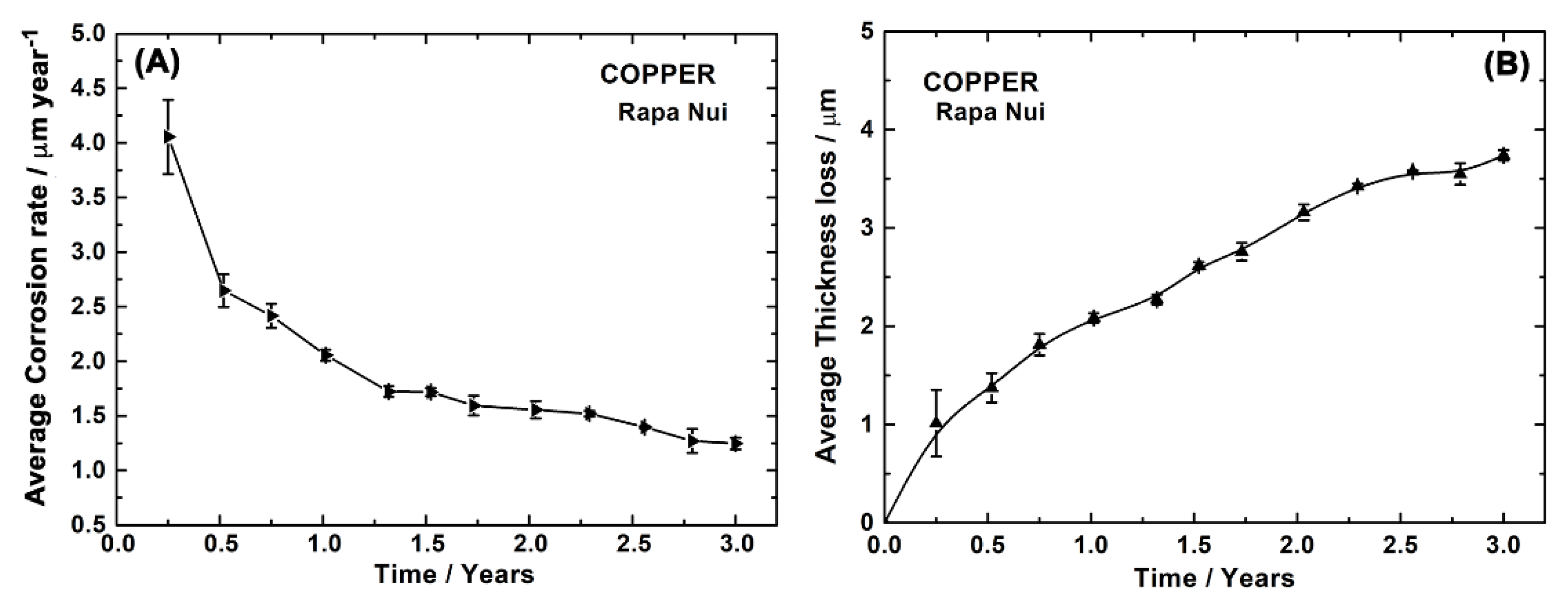
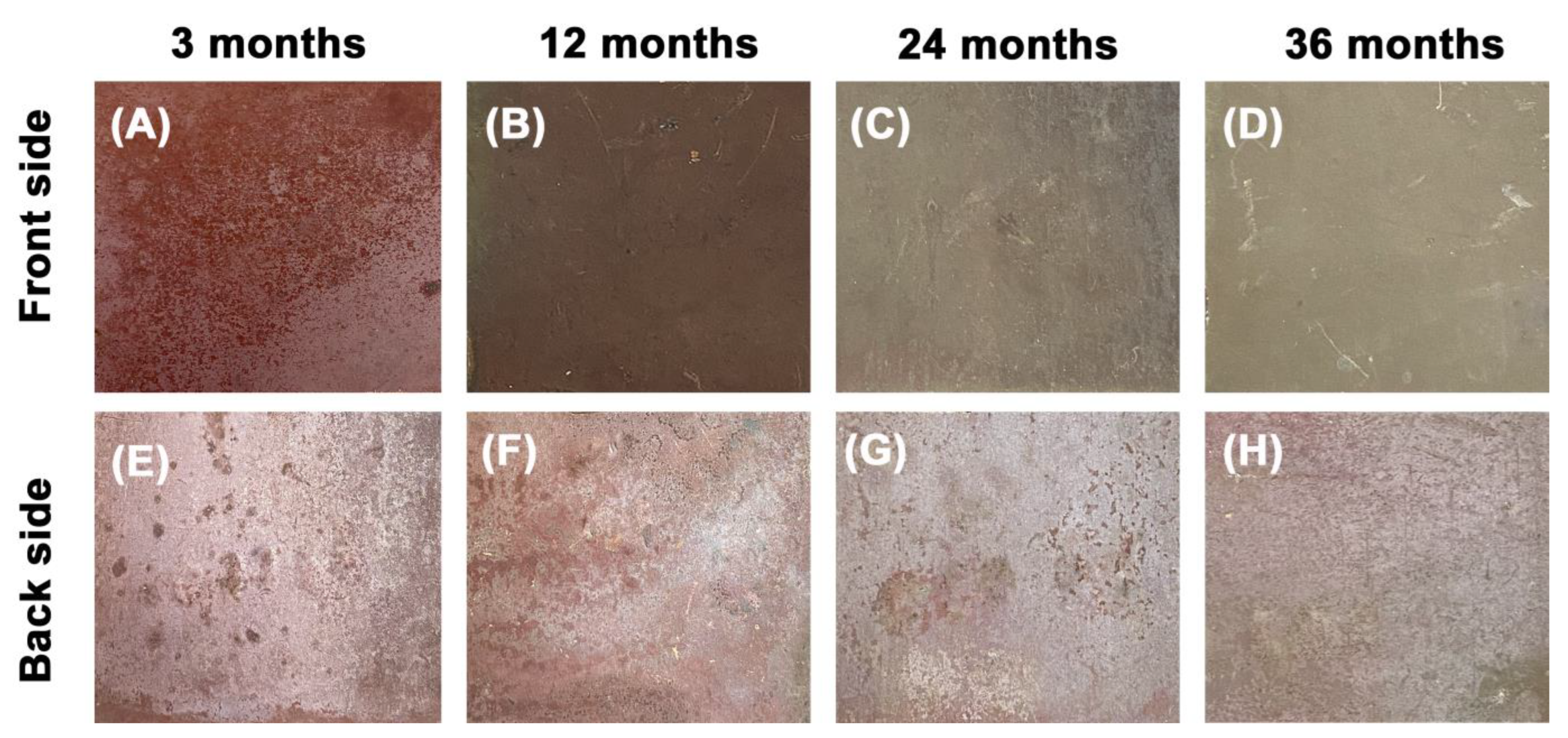
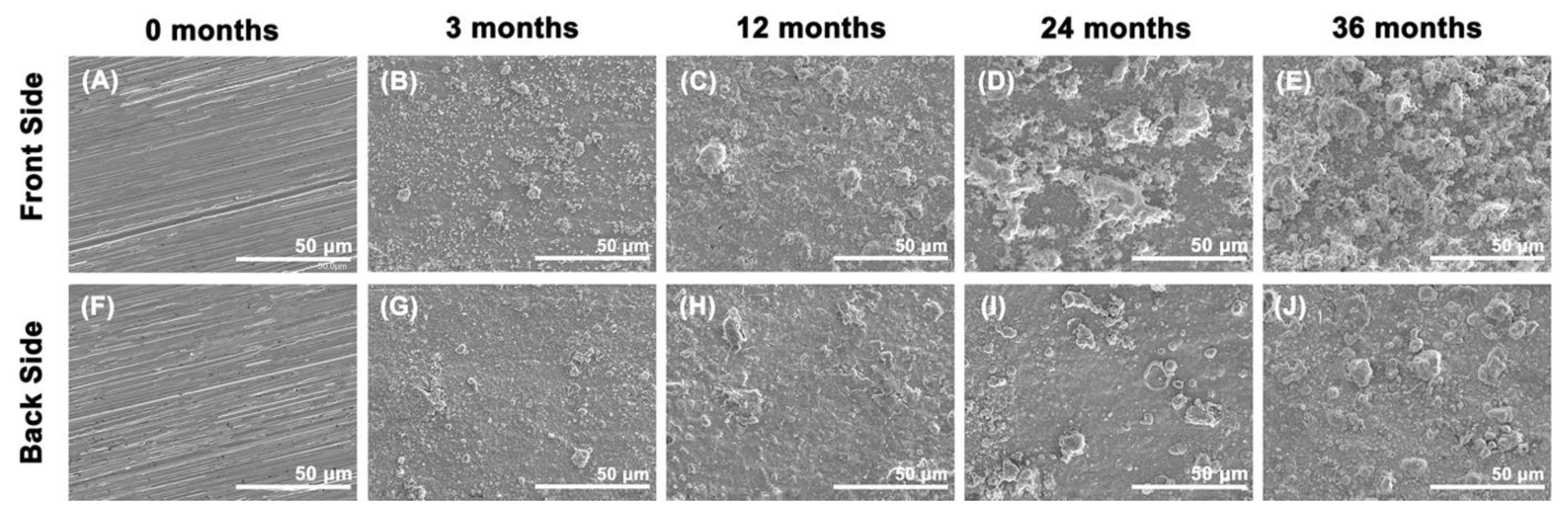
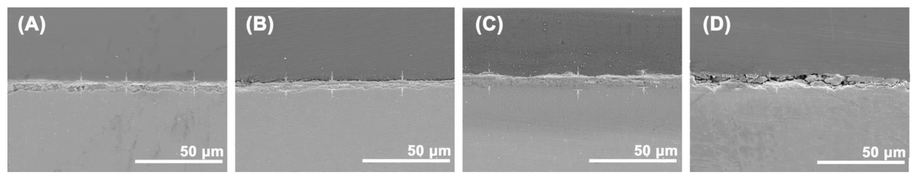
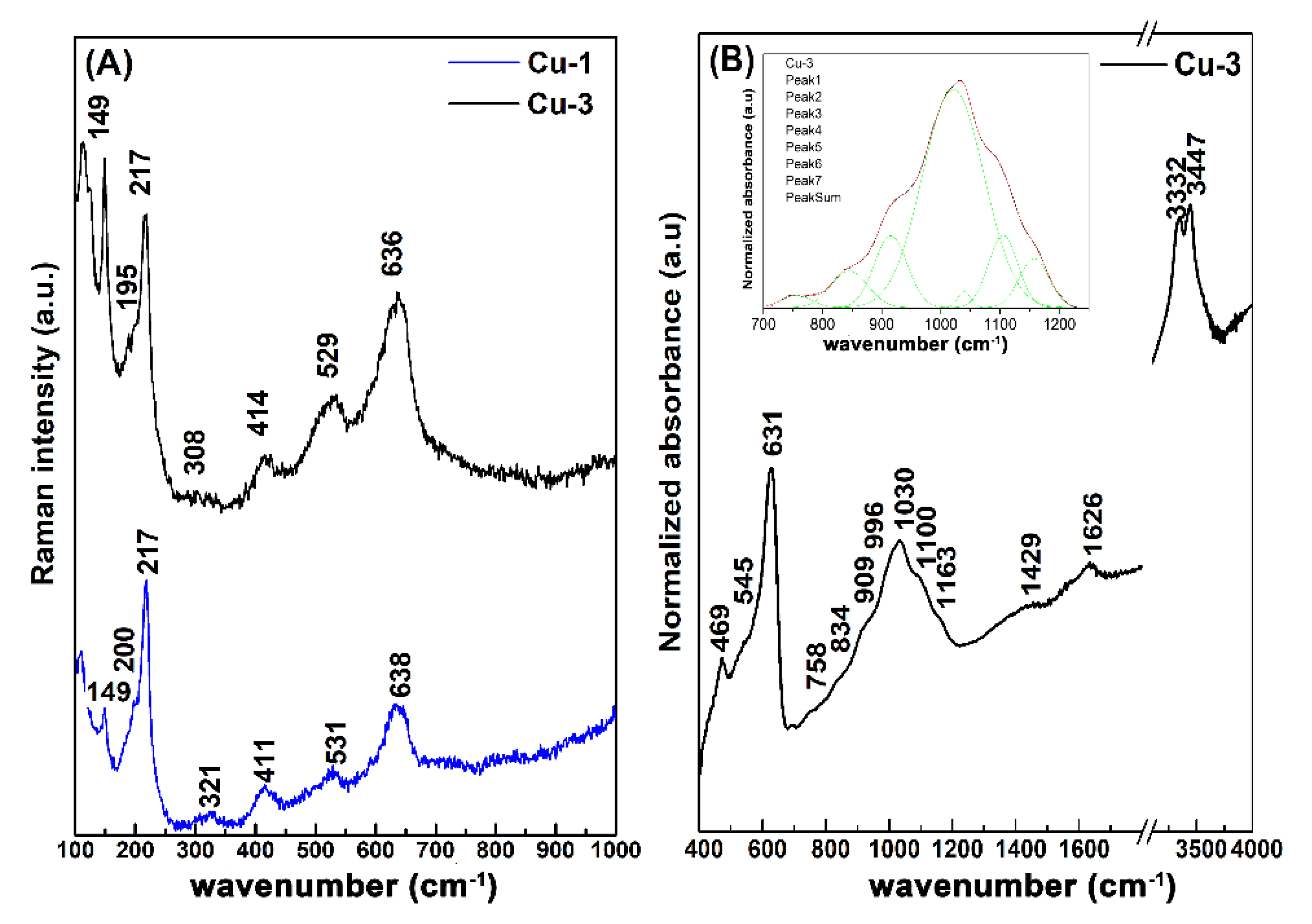
3.2. Corrosion Rate and Characteristics of Corrosion Products

Figure 6A,B shows the variations in the corrosion rate and loss of copper thickness as a function of exposure time, respectively. As seen here, as the exposure time increased, the corrosion rate decreased, and thickness loss increased. The decrease in corrosion rate can be divided into three states: rapid corrosion in the first cycle (between 3 and 6 months), which decreased the corrosion rate rapidly (approximately 35%); the second state, a deceleration in decrease of the corrosion rate, depending on the accumulation, type, and characteristics of the corrosion products protecting the surface of the metal from aggressive ions—in the case of copper, generally an internal cuprite layer (Cu₂ O) with basic chlorides on top sealing any pores on the cuprite layer [24]; and the third, a constant corrosion rate at 1.25 µm yr⁻¹ after three years of exposure, which was 69% less than at three months of exposure (4.05 µm yr⁻¹).

More specifically, the copper corrosion rate at one year of exposure was 2.10 µm yr⁻¹, which classifies as corrosivity category C4, according to ISO 9223 [32]. In this atmosphere, τ4S1P0, i.e., low average ambient chloride content (50.85 mg m⁻² d⁻¹), average SO₂ (3.53 mg m⁻² d⁻¹, and high wetting time, the behavior of copper depends mainly on the chloride concentration and wetting time. Some MICAT authors [1] mentioned that chloride concentrations above 20 mg m⁻² d⁻¹ create porous corrosion product structures, which, in turn, facilitate soluble salts retention and prevent rainwater entrainment; this thus increases conductivity in the formed corrosion product layer, increasing copper surface corrosion. Notably, however, the amount of rainfall increased during exposure time in this study, reaching a total rainfall of 2605 mm after three years of exposure.

The obtained copper corrosion rate (2.10 µm yr⁻¹) was similar to measurements from Camet Station (Argentina) in the MICAT project [1] (2.20 µm yr⁻¹), which had an average chloride content of 55.1 mg m⁻²d⁻¹. The Rapa Nui MICAT site (300 m from the coastal edge), on the other hand, had a copper corrosion rate of 1.86 µm yr⁻¹ at one year of exposure, classifying it—similar to this study—as corrosivity category C4 [1]. However, that site had a reported chloride concentration less than 50 mg m⁻²d⁻¹ (exact value not given), 1.15 mg SO₂ m⁻² d⁻¹, and no TOW value.

During the current measurement period, although the environmental SO₂ content tripled, its classification remained that of low contamination (P0). Given the increasing amounts of rainfall in the course of the study—and thus, contaminant flushing and TOW increase—a greater increase in the corrosion rate was not expected in comparison with the previous study (1988–1994).

The corrosion kinetics of copper under the study conditions can be described by the following empirical equation CR = Atⁿ, where CR is the magnitude of corrosion (loss of thickness) of the copper at t years, A is the measure of corrosion (loss of thickness) at the first year of exposure (t = 1), n is an indicator parameter of the physicochemical behavior of the corrosion layer and its interactions with the atmosphere, and t is the exposure time of the metal in years.

The function, then, for copper thickness loss following time exposed under study conditions (Figure 6B) is given by Equation (1):

CR_Cu = 2.0763 × t^0.5464 (R² = 99.18%)

(1)

where n—slightly higher than 0.5—indicates that the corrosion mechanism of copper likely corresponds to diffusion throughout the corrosion product layer. Here, the morphology and microstructure of the corrosion product film—and thus, its protective capacity—play an important role in the corrosion rate. Specifically, if the constant n is less than 1, it indicates that the corrosion products formed are protective and, for n greater than 1, an accelerated corrosion process, implying deadhesion or extreme porosity of the corrosion product film, a loss of material protection from atmospheric contaminants [40,41,42,43,44].

Next, the mechanism that explains the corrosion process is presented based on the results presented by several authors [24,45,46], and considering that the main compound formed corresponded to Cu₂O.

The dissolution of copper occurs by a redox process, according to the following reactions:

Oxidation reaction:

$$\mathrm{Cu}\to {\mathrm{Cu}}^{+}+{\mathrm{e}}^{-}$$

Reduction reaction:

$${\mathrm{O}}_2+2{\mathrm{H}}_2\mathrm{O}+4{\mathrm{e}}^{-}\to 4{\mathrm{OH}}^{-}$$

Overall reaction:

$$4\mathrm{Cu}+{\mathrm{O}}_2+2{\mathrm{H}}_2\mathrm{O}\to 4{\mathrm{Cu}}^{+}+4{\mathrm{OH}}^{-}$$

Subsequently, the Cu⁺ ion in the presence of chloride gives rise to the formation of CuCl (slightly soluble salt) and CuCl₂, where CuCl₂ by precipitation gives rise to the formation of Cu₂O [45].

$$2{\mathrm{Cu}}^{+}+4{\mathrm{Cl}}^{-}\to 2{\mathrm{CuCl}}_2^{-}$$

$$2{\mathrm{CuCl}}_2^{-}+2{\mathrm{OH}}^{-}\to {\mathrm{Cu}}_2\mathrm{O}+2{\mathrm{H}}_2\mathrm{O}+4{\mathrm{Cl}}^{-}$$

As a minor product, the presence of atacamite, formed after 3 years of exposure, was identified by Raman spectroscopy. This can be attributed to the low chloride concentrations reported [45].

$$3{\mathrm{CuCl}}_2^{-}+\frac{3}{4}{\mathrm{O}}_2+\frac{3}{2}{\mathrm{H}}_2\mathrm{O}\to {\mathrm{Cu}}_2{\left(\mathrm{OH}\right)}_3\mathrm{Cl}+{\mathrm{Cu}}^{2+}+5{\mathrm{Cl}}^{-}$$

Figure 7 shows the copper patina surfaces on both sides (e.g., differing copper sample orientations to the environment) at different exposure times. The back sides show less influence from contaminant deposition (mainly Cl ions⁻), the effect of rain by erosion, the effect of wind speed by abrasion, and the intensity of solar radiation. Indeed, more and more homogeneously distributed corrosion products were observed on the exposed face, while the nonexposed sides had a brittle corrosion product. Results that presented a similar trend were found by Wang et al. [47] when studying the corrosion of Ti coatings on brass and copper, where the greatest deterioration of the material occurred on the exposed face. After 3 months of exposure, the outward-facing corrosion product had a reddish-brown color and, after 36 months, a slight greenish color. This coloration is related to the formation of Cu₂O and basic copper chlorides [45].

Surface photographs (SEM) of the copper at 3, 12, 24, and 36 months of exposure are shown in Figure 8. The exposed sides show a nonhomogeneous granular corrosion product, with increasingly irregular growth throughout the years of exposure. The result is noncompact, rough structures, with elevations and depressions, which prevent, to some degree, the formation of protective films. The unexposed sides show a more irregular and disorderly growth and less corrosion products than the exposed side; however, the corrosion product continues to increase as a function of exposure time. These results were expected given the low environmental pollutant content (S1P0) and the total amount of rainfall during the study period.

Table 2. EDS of the copper corrosion product at different exposure times. 1000$\times$.

Atom %	3 Months		12 Months		24 Months		36 Months
	Front Side	Back Side	Front Side	Back Side	Front Side	Back Side	Front Side	Back Side
Copper	69.65	64.74	47.11	56.23	34.88	41.41	27.09	43.38
Oxygen	32.81	29.01	47.36	38.61	54.56	46.76	62.84	50.53
Chlorine	1.34	2.45	5.53	5.16	10.07	8.08	10.56	9.86

presents the semi-quantitative surface analysis (EDS) of copper corrosion products from Figure 8. As the exposure times increased, the copper content decreased while the oxygen content increased—for both exposed and unexposed faces—corroborating the presence of copper oxide in the corrosion product. However, the oxygen content was always lower on the unexposed side, indicating lower corrosion product formation compared to the exposed side. The chloride content also increased for both faces with the exposure time, though at a reduced rate for the exposed face at 24 and 36 months; this is likely due to higher rainfall rinsing soluble chlorides from the corrosion product. In sum, however, the chloride content was generally lower on the unexposed side, due to the shielding of the sample from the environment.

However, for the 3 months of exposure, this relationship was not fulfilled due to the amount of rain that fell during that time (291.2 mm), which generates the washing of the soluble chlorides on the exposed face. It is important to note that the conditions that favor the washing of surface chlorides are that, during this exposure time, the formation of corrosion products is less, and some areas of the sample surface are still smooth.

Next, cross-sectional photographs (Figure 9) show a serrated copper surface, with broad attacks. The average corrosion product thickness increased with the exposure time, reaching 3.49 ± 0.3 µm at 3 months, 5.19 ± 0.6 µm at 12 months, 8.27 ± 0.4 µm at 24 months, and 9.13 ± 0.5 µm at 36 months. The corrosion product layer presented cracks and pores, with occasional small adhesion losses, which allowed contaminants and increased the corrosion attack surface. Indeed, in the third year of exposure, there was an irregular, rough corrosion product layer, with elevations and depressions, that showed the loss of patina adherence in some areas (Figure 9D). In short, patina morphology under these conditions does not suggest a completely protective compact film. Furthermore, and as mentioned previously, layer roughness and porosity impede soluble salt removal by rainwater, thus encouraging greater corrosion rates and lending to the C4 corrosivity category.

The GD-OES depth profiles of copper samples exposed at Rapa Nui for 1 and 3 years corroborate thin oxide films formed on the copper surface. Notably, this technique did not find detachment or exfoliation of the corrosion product film on copper samples, even though SEM cross-section photographs (Figure 9) showed cracks in the corrosion product.

Next, X-ray diffraction determined the main copper corrosion product to be cuprite (Cu₂O). This is in line with Lopesino et al. [24], who found that the inner corrosion product layer in coastal zones was cuprite, as well as with Pan et al. [30], who found inner layers of cuprite corrosion in simulated coastal–industrial atmospheres, as well as in the atmospheric corrosion of copper in the middle of H₂S [48]. In a study in the Nansha Islands, China, Lu et al. [45] determined that the composition of the inner layer of the corrosion product corresponded to Cu₂O, with a very thin outer layer of mainly Cu₂ Cl(OH)₃, at a corrosion rate of 7.85 µm per year⁻¹ (corrosivity category CX).

Corrosion products formed on copper exposed to the environment were also identified using the Raman technique at 1 and 3 years. Bands between 140 and 650 cm⁻¹ were related to the presence of cuprite (Cu₂O), and, after three years of exposure, the IR spectrum showing three bands centered at 631, 545, and 469 cm⁻¹ showed it as the main corrosion product, consistent with Zhang [28]. A wide band of seven components was also observed between 1250 and 750 cm⁻¹, with four peaks centered around 1030, 996, 906, and 835 cm⁻¹. These were assigned to deformations of the (-OH) group. In turn, two vibrations at 3332 and 3447 cm⁻¹ were associated with deformations in (O-H); this set of signals implies small amounts of atacamite (Cu₂Cl(OH)₃) as a corrosion product, consistent with the exposure of the sample to a marine environment (Figure 10) [1,49] and with the slight green hue presented by the patina in the sample exposed after 3 years of exposure (Figure 7D). Literature references [45] indicated that the stability of Cu₂O is inversely dependent on the chloride concentration; given the environmental chloride content of the study site in Rapa Nui is 58 mg m⁻² d⁻¹ (category S1), the formation of cuprite was expected as the main corrosion product.

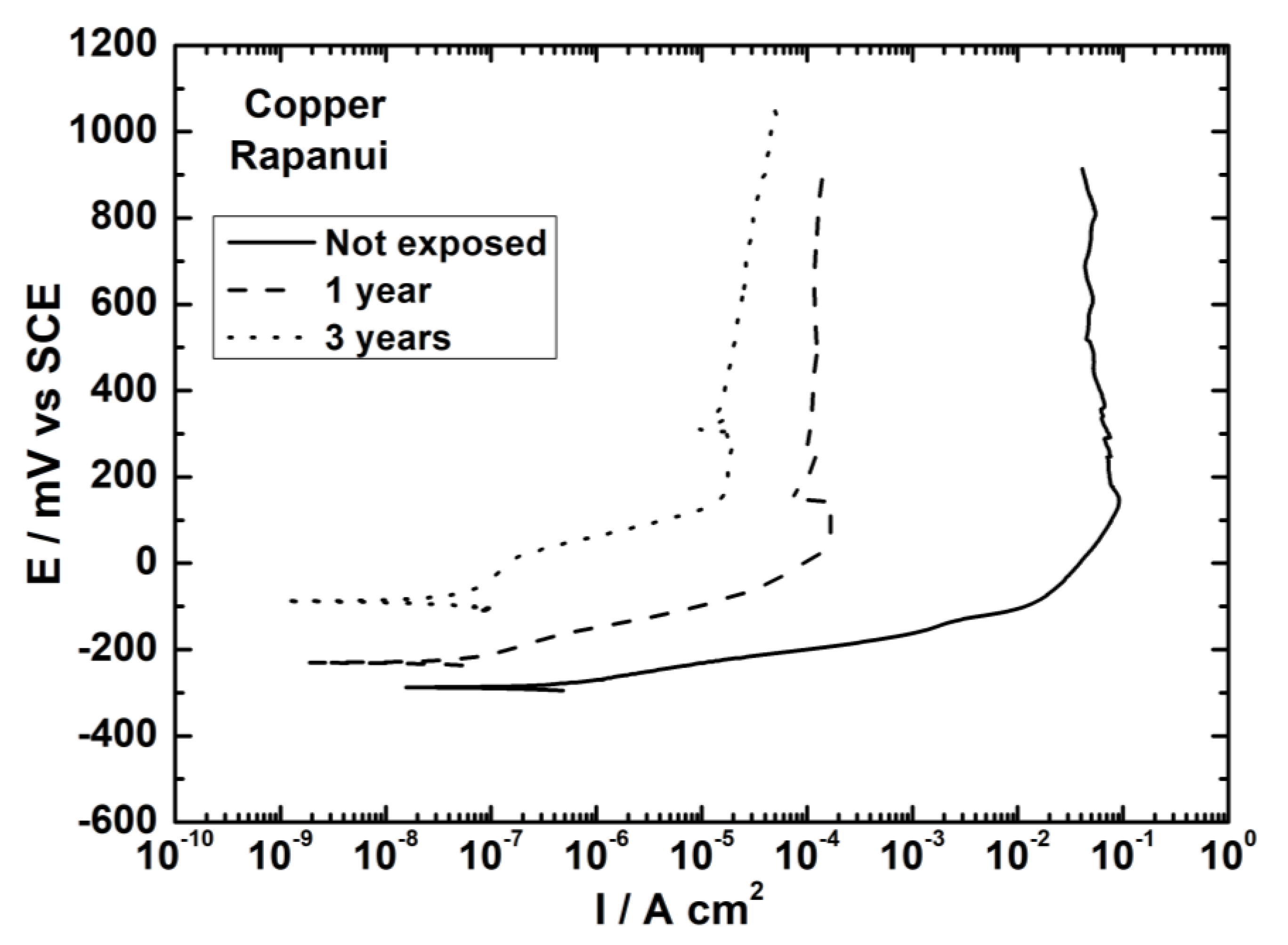
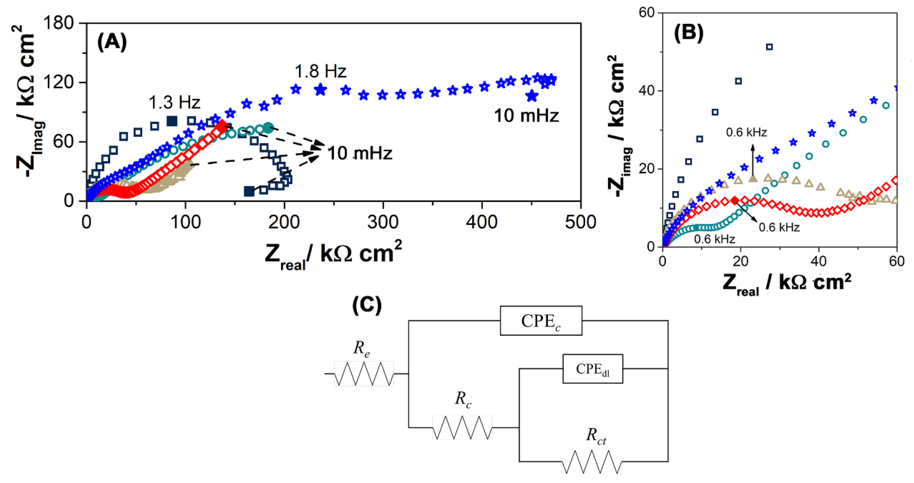
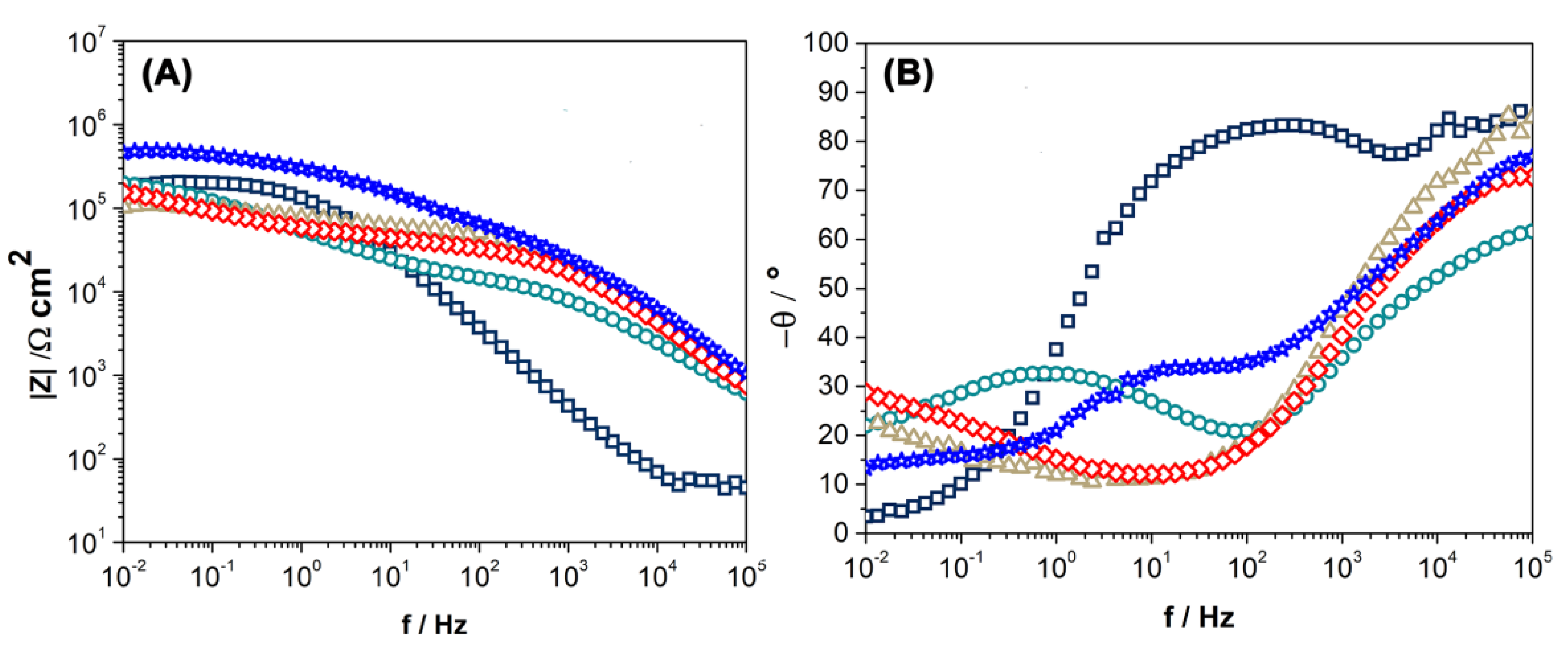
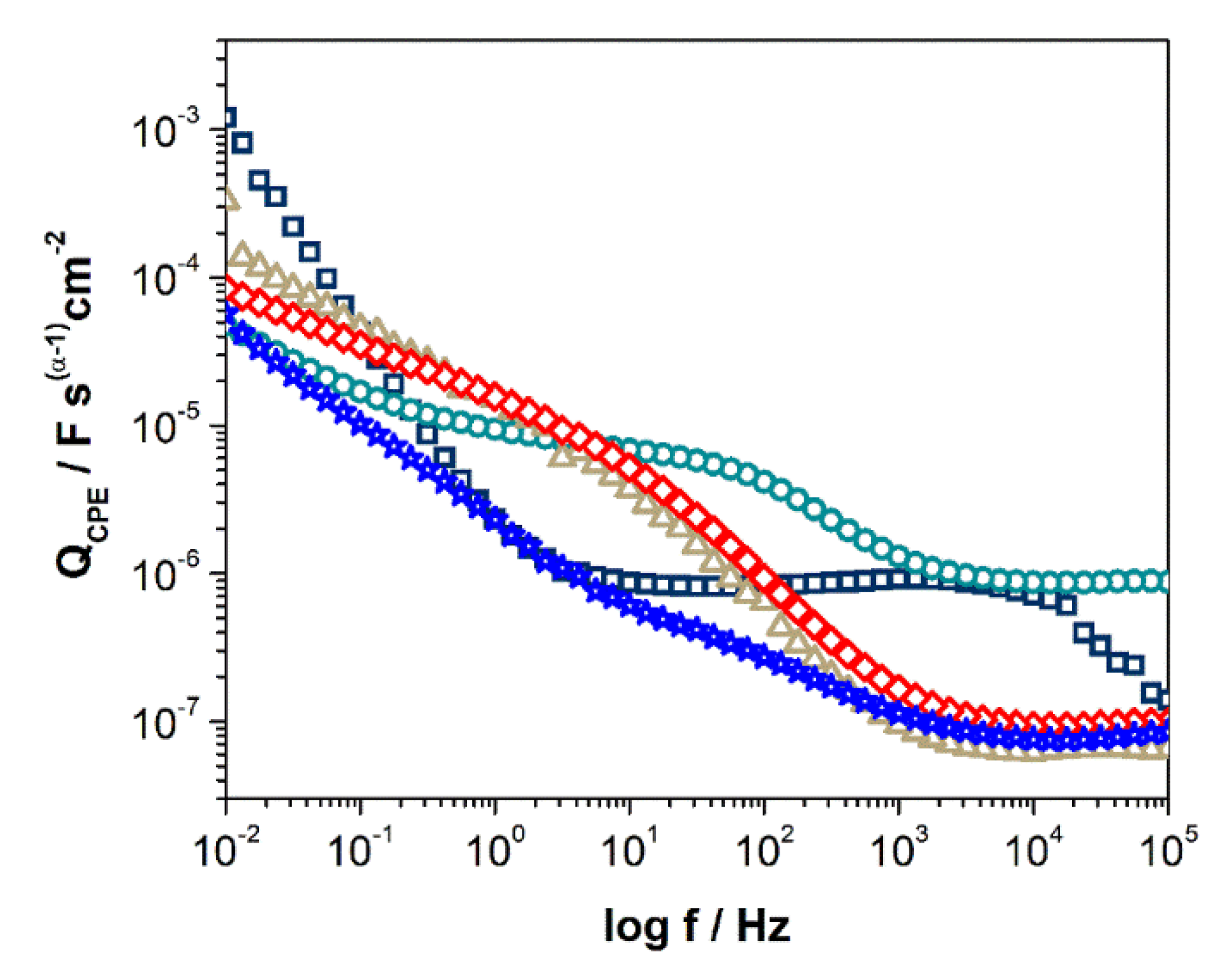
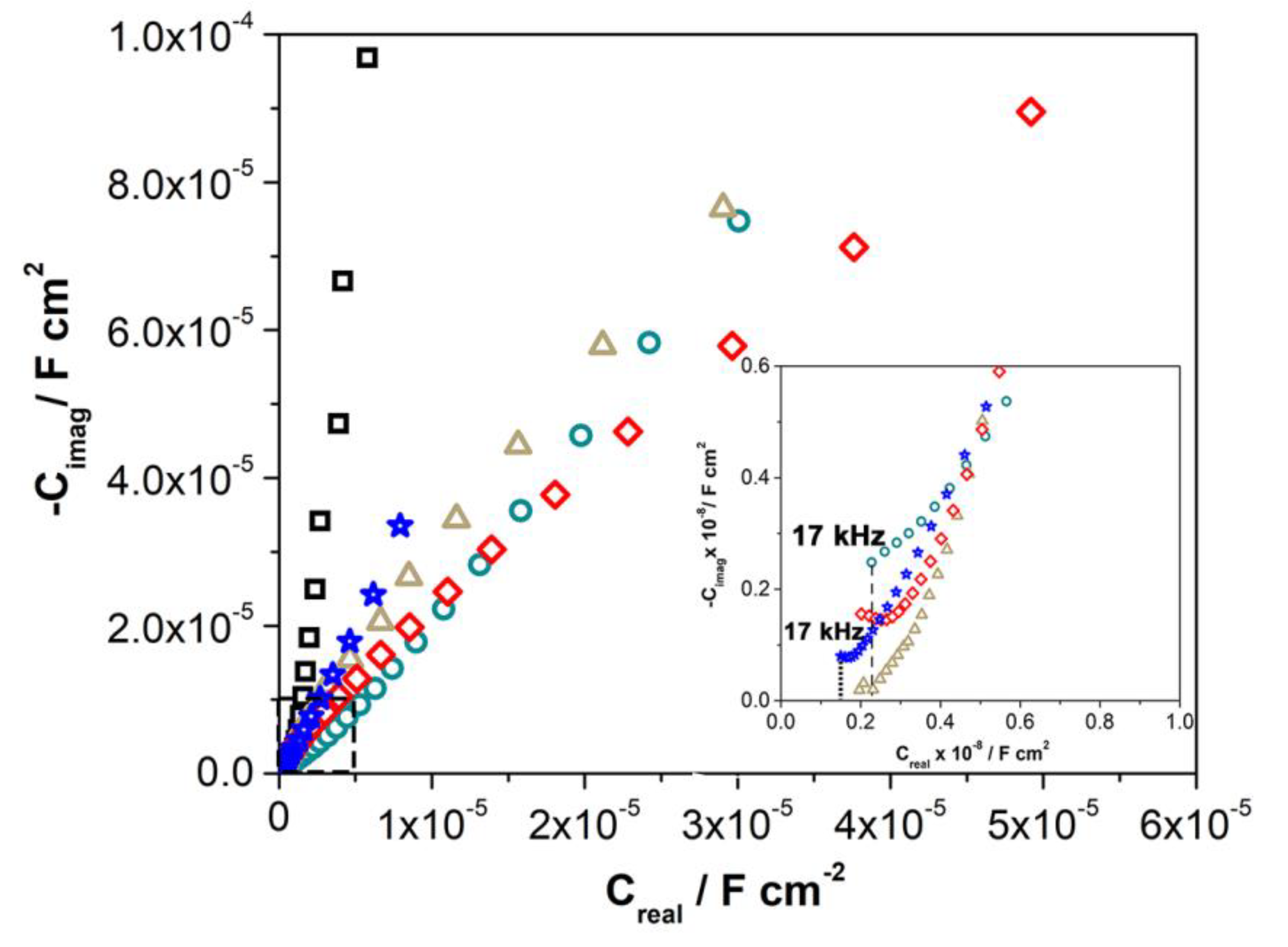
3.3. Electrochemical Measurements

The protective capability of corrosion products on the copper was analyzed by plotting the respective anodic curves in a 0.1 M Na₂SO₄ solution for unexposed and environmentally exposed probes (back and front sides) after one and three years. Figure 11 shows a general increase in corrosion potential and a decrease in active and passive dissolution zone current density as a function of exposure time. The corrosion potential of the bare metal began at −288.9 mVsce and moved, after one year of exposure, to −230.5 mVsce, increasing by 58.4 mVsce. After three years, the corrosion potential was −92.7 mVsce; with respect to unexposed copper, an increase of 196.2 mVsce; and, to copper corrosion products after one year, of 137.8 mVsce. The increased corrosion potential corroborated the formation of a corrosion product layer that increased in thickness as a function of exposure time (Figure 9).

These variations further confirm that cuprite formation in marine environments resulted in porous, cracked, and nonuniformly distributed morphology on the surface of the metal, i.e., characteristics that reduced the protection capabilities. This allowed a corrosion attack from chloride to continue on copper, increasing the thickness of the layer; however, the Raman analysis in year three detected the presence of Cu₂Cl(OH)₃, which, in accordance with the results from previous studies on basic chlorides [1,45,49], may have sealed the cuprite pores and achieved more protective properties. This was indeed the case, corroborated by anode plots that showed a decrease in the current as a function of exposure time. Measurements showed an anodic current of 6.08 × 10⁻² A cm⁻² for unexposed copper, 1.13 × 10⁻⁴ A cm⁻² for copper exposed for one year, and 1.69 × 10⁻⁵ A cm⁻² for three years exposure time. This plot further shows that the active dissolution zone of the unexposed copper decreased with increased thickness (and, thus, protective character) of the corrosion product layer formed during the exposure time.

Figure 12 shows the Nyquist plot response in 0.1 M Na₂SO₄ solution of copper samples exposed to the environment after three years (front side). All samples showed nonideal capacitive behavior at full frequencies due to their current and potential distribution over the surface [49], which revealed a constant phase element (CPE) behavior that can be represented by CPE parameters Q_CPE and α. Figure 12C shows the proposed equivalent circuit, where CPE_C and CPE_dl correspond to the capacitances of the oxide and the electrical double layer, respectively. In addition, Re represents the electrolyte resistance, R_C corresponds to the oxide resistance, and Rct represents the resistance to the charge transfer occurring at the oxide/metal interface.

The Bode diagram, presented in Figure 13, suggests the formation of an oxide layer, which increased with the exposure time, showing a higher modulus (Figure 13A) at 36 months of exposure. However, the decrease in the phase constant after 24 months of exposure (Figure 13B) suggests that the layer loses protectiveness with time, which could be due to a loss of homogeneity in the film.

The CPE parameters related to the corrosion product properties, estimated by the graphic method, are summarized in

Table 3. Impedance parameters of copper samples at different exposure times.

t (months)	Re (Ωcm2)	−αHF	${\mathbf{Q}}_{\mathbf{eff},\mathbf{HF}}\times {10}^{-8} \left(\mathbf{F}{\mathbf{S}}^{\left(\mathit{\alpha }-1\right)}\mathbf{c}{\mathbf{m}}^{-2}\right)$	${\mathbf{C}}_{\text{∞}}\times {10}^{-9}$$(\mathbf{F}\mathbf{c}{\mathbf{m}}^{-2})$
0	338	0.89	89.1	12.1
3	188	0.55	87.1	1.35
12	245	0.73	6.2	2.16
24	336	0.71	9.6	1.38
36	244	0.69	7.4	1.17

. The CPE behavior associated with the oxide film in the high frequency (HF) zones at 3 months of exposure presented a value of around 0.55 and a Q_CPE coefficient close to 8.71 × 10⁻⁷ (F·s^(α−1)·cm⁻²), which—although of a higher frequency—was very similar to that of the unexposed copper sample (8.91 × 10⁻⁷ (F·s^(α−1)·cm⁻²)). This continues to suggest the formation of the cuprite oxide layer, in agreement with behaviors for the estimated constant phase element (CPE) values as the exposure time increased [50,51].

Figure 14 shows how parameter Q_eff decreased more than tenfold after a year of exposure, which suggests an increase in the protective capacity of the oxide film formed on the surface [51]. However, as shown in Table 3, Q_eff values denoted lost protectiveness at 2 and 3 years, which suggests that the oxide film was not homogeneous, nor compact, as in Xiao Lu et al. [45].

The infinite capacitances (C_∞) were estimated from the Cole–Cole diagram [52,53] for copper samples exposed to the environment for up to 36 months, as shown in Figure 15. The segmented lines represent the criteria used in the determination of C_∞, giving by extrapolation the real capacitance (C_real) using the slope of the complex capacitance at HF. In addition, Figure 15 shows the variation of C_∞ obtained from the extrapolation line with a positive slope for all the evaluated systems, revealing that the highest value of C_∞ was presented by pure copper samples before exposure, while those exposed at different times decrease by orders of magnitude. From C_∞, the oxide thickness was estimated as previously described by A. S. Nguyen [53], and B. Tribollet [52].

$${\mathrm{C}}_{\infty }=\frac{{\mathsf{\epsilon }\mathsf{\epsilon }}_0}{\mathrm{d}}$$

(2)

where C_∞ is the capacitance in F∙cm⁻², d is the oxide thickness in cm, ε₀ is the vacuum permittivity (ε₀ = 8.8542 × 10⁻¹⁴ F cm⁻¹), and ε is the dielectric constant of the Copper I (Cu₂O) oxide layer corresponding to ε = 7.6 [52].

The oxide film thickness estimations from the GD-OES, SEM, and impedance analysis after exposure to the electrolyte are summarized in

Table 4. Variations of copper oxide thicknesses on the exposed metal surface.

Exposure Condition, Months	3	12	24	36
Thickness (µm) by GD-OES	1.6	---	---	6.3
Thickness (µm) by SEM	3.5	5.2	8.3	9.1
Thickness (µm), Graphically	4.9	3.1	4.9	5.8

. The differences are broadly attributable to technique precision, and the SEM analysis was performed locally and so may have been strongly influenced by the lack of film homogeneity. At 36 months of exposure, all techniques showed increased film thickness, independent of the irregularity or porosity presented by the copper oxide film formed (Figure 9D), as has been previously reported on typical cuprite behavior [45]. Notwithstanding, the impedance analysis suggested that the copper oxide film thickness was 3.1 < d < 5.8 μm. The thickness was almost constant up to 24 months and increased after 36 months, which may be since defects, porosity, cracks, and irregularities of the film through 12 months of exposure to 24 months were lesser, therefore favoring the migration of ions to the metal–oxide interface (Figure 9D).

4. Conclusions

Twenty-two years after the MICAT project on Rapa Nui Island, this study updates the behavior of copper against corrosion, considering the changes in global warming and in the contents of pollutants, and shows that the copper corrosion rate increased by 11.0% in spite of the higher elevation and greater coastal distance of the exposure zone in this study. Additionally, the environmental SO₂ deposition was three times higher than 22 years ago, mainly associated with the increased local population and continuous tourist presence on the island. In both study periods, the corrosion rate of exposed copper in Rapa Nui was classified in corrosivity category C4.

The main compound present in copper patinas was found to be cuprite (Cu₂O), with porous, nonhomogeneous, and thin morphology results similar to those obtained in research carried out 22 years ago. In this study, after 36 months of exposure, a minor amount of atacamite (Cu₂Cl(OH)₃) was also detected. The exposed sides of the copper probes presented greater, more homogeneously distributed corrosion products than on the nonexposed sides, which presented a brittle corrosion product.

The electrochemical results showed that anodic polarization curves from the front (exposed) faces have a higher corrosion potential and decreased current density in the active and passive dissolution zones as a function of the exposure time. Although this corroborates increases in the corrosion product layer thickness as a function of exposure time, this thin layer of copper oxide (Cu₂O) was shown to lose its protective capacity after its maximum at a year of exposure time due to increased irregularities.

References

1. Morcillo, M.; Almeida, E.; Rosales, B.; Uruchurtu, J.; Marrocos, M. Corrosion y Proteccion de Metales En Las Atmosferas de Iberoamerica, Parte I; CYTED: Cambridge, UK, 1998; ISBN 8493044814. [Google Scholar]
2. Morcillo, M.; Díaz, I.; Cano, H.; Chico, B.; de la Fuente, D. Atmospheric Corrosion of Weathering Steels. Overview for Engineers. Part I: Basic Concepts. Constr. Build. Mater. 2019, 213, 723–737. [Google Scholar] [CrossRef]
3. Morcillo, M.; Díaz, I.; Cano, H.; Chico, B.; de la Fuente, D. Atmospheric Corrosion of Weathering Steels. Overview for Engineers. Part II: Testing, Inspection, Maintenance. Constr. Build. Mater. 2019, 222, 750–765. [Google Scholar] [CrossRef]
4. Morcillo, M.; Chico, B.; de la Fuente, D.; Almeida, E.; Joseph, G.; Rivero, S.; Rosales, B. Atmospheric Corrosion of Reference Metals in Antarctic Sites. Cold Reg. Sci. Technol. 2004, 40, 165–178. [Google Scholar] [CrossRef] [Green Version]
5. Morcillo, M.; Chico, B.; de la Fuente, D.; Simancas, J. Looking Back on Contributions in the Field of Atmospheric Corrosion Offered by the MICAT Ibero-American Testing Network. Int. J. Corros. 2012, 2012, 1–24. [Google Scholar] [CrossRef] [Green Version]
6. Morcillo, M.; Chico, B.; Díaz, I.; Cano, H.; de la Fuente, D. Atmospheric Corrosion Data of Weathering Steels. A Review. Corros. Sci. 2013, 77, 6–24. [Google Scholar] [CrossRef] [Green Version]
7. Morales, J.; Díaz, F.; Hernández-Borges, J.; González, S. Atmospheric Corrosion in Subtropical Areas: XRD and Electrochemical Study of Zinc Atmospheric Corrosion Products in the Province of Santa Cruz de Tenerife (Canary Islands, Spain). Corros. Sci. 2006, 48, 361–371. [Google Scholar] [CrossRef]
8. Vidal, F.; Vicente, R.; Mendes Silva, J. Review of Environmental and Air Pollution Impacts on Built Heritage: 10 Questions on Corrosion and Soiling Effects for Urban Intervention. J. Cult. Herit. 2019, 37, 273–295. [Google Scholar] [CrossRef]
9. de la Fuente, D.; Alcántara, J.; Chico, B.; Díaz, I.; Jiménez, J.A.; Morcillo, M. Characterisation of Rust Surfaces Formed on Mild Steel Exposed to Marine Atmospheres Using XRD and SEM/Micro-Raman Techniques. Corros. Sci. 2016, 110, 253–264. [Google Scholar] [CrossRef]
10. Alcántara, J.; Chico, B.; Simancas, J.; Díaz, I.; de la Fuente, D.; Morcillo, M. An Attempt to Classify the Morphologies Presented by Different Rust Phases Formed during the Exposure of Carbon Steel to Marine Atmospheres. Mater. Charact. 2016, 118, 65–78. [Google Scholar] [CrossRef]
11. Vera, R.; Rosales, B.M.M.; Tapia, C. Effect of the Exposure Angle in the Corrosion Rate of Plain Carbon Steel in a Marine Atmosphere. Corros. Sci. 2003, 45, 321–337. [Google Scholar] [CrossRef]
12. Vera, R.; Rincón, O.T.; Ramirez, J.; Valverde, B.; Díaz-Gómez, A.; Sánchez-González, R. Effect of Height on the Corrosion of Steel and Galvanized Steel in Nontropical Coastal Marine Environments. Mater. Corros. 2020, 71, 1125–1137. [Google Scholar] [CrossRef]
13. Vera, R.; Puentes, M.; Araya, R.; Rojas, P.; Carvajal, A. Mapa de Corrosión Atmosférica de Chile : Resultados Después de Un Año de Exposición. Revista de la Construcción 2012, 11, 61–72. [Google Scholar] [CrossRef] [Green Version]
14. Vera, R.; Delgado, D.; Araya, R.; Puentes, M.; Guerrero, I.; Rojas, P.; Cabrera, G.; Erazo, S.; Carvajal, A.M. Construcción de Mapas de Corrosión Atmosférica de Chile: Resultados Preliminares. Rev. Latinoam. Metal. y Mater. 2012, 32, 269–276. [Google Scholar]
15. Carvajal, M.; Winckler, P.; Garreaud, R.; Igualt, F.; Contreras-López, M.; Averil, P.; Cisternas, M.; Gubler, A.; Breuer, W.A. Extreme Sea Levels at Rapa Nui (Easter Island) during Intense Atmospheric Rivers. Nat. Hazards 2021, 106, 1619–1637. [Google Scholar] [CrossRef]
16. An, S.-I.; Park, H.-J.; Kim, S.-K.; Shin, J.; Yeh, S.-W.; Kug, J.-S. Intensity Changes of Indian Ocean Dipole Mode in a Carbon Dioxide Removal Scenario. npj Clim. Atmos. Sci. 2022, 5, 20. [Google Scholar] [CrossRef]
17. Rull, V. Contributions of Paleoecology to Easter Island’s Prehistory: A Thorough Review. Quat. Sci. Rev. 2021, 252, 106751. [Google Scholar] [CrossRef]
18. Castañeda, A.; Valdés, C.; Corvo, F. Atmospheric Corrosion Study in a Harbor Located in a Tropical Island. Mater. Corros. 2018, 69, 1462–1477. [Google Scholar] [CrossRef]
19. Corvo, F.; Perez, T.; Dzib, L.R.; Martin, Y.; Castañeda, A.; Gonzalez, E.; Perez, J. Outdoor–Indoor Corrosion of Metals in Tropical Coastal Atmospheres. Corros. Sci. 2008, 50, 220–230. [Google Scholar] [CrossRef]
20. de la Fuente, D.; Díaz, I.; Simancas, J.; Chico, B.; Morcillo, M. Long-Term Atmospheric Corrosion of Mild Steel. Corros. Sci. 2011, 53, 604–617. [Google Scholar] [CrossRef] [Green Version]
21. Santana, J.J.; Ramos, A.; Rodriguez-Gonzalez, A.; Vasconcelos, H.C.; Mena, V.; Fernández-Pérez, B.M.; Souto, R.M. Shortcomings of International Standard Iso 9223 for the Classification, Determination, and Estimation of Atmosphere Corrosivities in Subtropical Archipelagic Conditions—The Case of the Canary Islands (Spain). Metals 2019, 9, 1105. [Google Scholar] [CrossRef] [Green Version]
22. Lo, C.M.; Tsai, L.H.; La, H.H.; Wu, W.T.; Lin, M.D. A Study on the Metallic Corrosion Characteristics under Atmospheric Environment in Taiwan: Taking Taichung Harbor as an Example. Mater. Corros. 2018, 69, 251–265. [Google Scholar] [CrossRef]
23. Vera, R.; Araya, R.; Bagnara, M.; Díaz-Gómez, A.; Ossandón, S. Atmospheric Corrosion of Copper Exposed to Different Environments in the Region of Valparaiso, Chile. Mater. Corros. 2017, 68, 316–328. [Google Scholar] [CrossRef]
24. Lopesino, P.; Alcántara, J.; de la Fuente, D.; Chico, B.; Jiménez, J.; Morcillo, M. Corrosion of Copper in Unpolluted Chloride-Rich Atmospheres. Metals 2018, 8, 866. [Google Scholar] [CrossRef] [Green Version]
25. Rosales, B.M.; Vera, R.M.; Hidalgo, J.P. Characterisation and Properties of Synthetic Patina on Copper Base Sculptural Alloys. Corros. Sci. 2010, 52, 3212–3224. [Google Scholar] [CrossRef]
26. Franey, J.P.; Davis, M.E. Metallographic Studies of the Copper Patina Formed in the Atmosphere. Corros. Sci. 1987, 27, 659–668. [Google Scholar] [CrossRef]
27. Chang, T.; Wallinder, I.O.; de la Fuente, D.; Chico, B.; Morcillo, M.; Welter, J.M.; Leygraf, C. Analysis of Historic Copper Patinas. Influence of Inclusions on Patina Uniformity. Materials 2017, 10, 298. [Google Scholar] [CrossRef] [PubMed] [Green Version]
28. Zhang, X.; Odnevall Wallinder, I.; Leygraf, C. Mechanistic Studies of Corrosion Product Flaking on Copper and Copper-Based Alloys in Marine Environments. Corros. Sci. 2014, 85, 15–25. [Google Scholar] [CrossRef] [Green Version]
29. Morcillo, M.; Chang, T.; Chico, B.; de la Fuente, D.; Odnevall Wallinder, I.; Jiménez, J.A.; Leygraf, C. Characterisation of a Centuries-Old Patinated Copper Roof Tile from Queen Anne’s Summer Palace in Prague. Mater. Charact. 2017, 133, 146–155. [Google Scholar] [CrossRef]
30. Pan, C.; Lv, W.; Wang, Z.; Su, W.; Wang, C.; Liu, S. Atmospheric Corrosion of Copper Exposed in a Simulated Coastal-Industrial Atmosphere. J. Mater. Sci. Technol. 2017, 33, 587–595. [Google Scholar] [CrossRef]
31. Mendoza, A.R.; Corvo, F.; Gómez, A.; Gómez, J. Influence of the Corrosion Products of Copper on Its Atmospheric Corrosion Kinetics in Tropical Climate. Corros. Sci. 2004, 46, 1189–1200. [Google Scholar] [CrossRef]
32. ISO 9223:2012; Corrosion of Metals and Alloys. Corrosivity of Atmospheres. Classification, Determination and Estimation. International Organization for Standardization: Geneva, Switzerland, 2008.
33. ISO 9224:2012; Corrosion of Metals and Alloys-Corrosivity of Atmospheres-Guiding Values for the Corrosivity Categories. International Organization for Standardization: Geneva, Switzerland, 2012.
34. ISO 9225:2012; Corrosivity of Atmospheres-Measurement of Environmental Parameters Affecting Corrosivity of Atmospheres. International Organization for Standardization: Geneva, Switzerland, 2012.
35. ISO 9226:2012; Corrosion of Metals and Alloys-Corrosivity of Atmospheres-Determination of Corrosion Rate of Standard Specimens for the Evaluation of Corrosivity. International Organization for Standardization: Geneva, Switzerland, 2012.
36. ASTM G1−03; Standard Practice for Preparing, Cleaning, and Evaluating Corrosion Test Specimens. ASTM Special Technical Publication: West Conshohocken, PA, USA, 2017; pp. 505–510.
37. ASTM G50-20; Standard Practice for Conducting Atmospheric Corrosion Tests on Metals. ASTM Special Technical Publication: West Conshohocken, PA, USA, 2020; Volume 1, pp. 1–6.
38. Chilean Navy Hydrographic and Oceanografic Service. Available online: http://www.shoa.cl/php/index.php (accessed on 22 April 1999 and 15 May 2015).
39. Schindelholz, E.; Kelly, R.G.; Cole, I.S.; Ganther, W.D.; Muster, T.H. Comparability and Accuracy of Time of Wetness Sensing Methods Relevant for Atmospheric Corrosion. Corros. Sci. 2013, 67, 233–241. [Google Scholar] [CrossRef]
40. Panchenko, Y.M.; Marshakov, A.I.; Igonin, T.N.; Kovtanyuk, V.V.; Nikolaeva, L.A. Long-Term Forecast of Corrosion Mass Losses of Technically Important Metals in Various World Regions Using a Power Function. Corros. Sci. 2014, 88, 306–316. [Google Scholar] [CrossRef]
41. Kreislova, K.; Geiplova, H. Prediction of the Long-Term Corrosion Rate of Copper Alloy Objects. Mater. Corros. 2016, 67, 152–159. [Google Scholar] [CrossRef]
42. Panchenko, Y.M.; Marshakov, A.I. Long-Term Prediction of Metal Corrosion Losses in Atmosphere Using a Power-Linear Function. Corros. Sci. 2016, 109, 217–229. [Google Scholar] [CrossRef]
43. Ma, X.Z.; Meng, L.D.; Cao, X.K.; Zhang, X.X.; Dong, Z.H. Investigation on the Initial Atmospheric Corrosion of Mild Steel in a Simulated Environment of Industrial Coastland by Thin Electrical Resistance and Electrochemical Sensors. Corros. Sci. 2022, 204, 110389. [Google Scholar] [CrossRef]
44. Gießgen, T.; Mittelbach, A.; Höche, D.; Zheludkevich, M.; Kainer, K.U. Enhanced Predictive Corrosion Modeling with Implicit Corrosion Products. Mater. Corros. 2019, 70, 2247–2255. [Google Scholar] [CrossRef]
45. Lu, X.; Liu, Y.; Zhao, H.; Pan, C.; Wang, Z. Corrosion Behavior of Copper in Extremely Harsh Marine Atmosphere in Nansha Islands, China. Trans. Nonferrous Met. Soc. China 2021, 31, 703–714. [Google Scholar] [CrossRef]
46. Liao, X.; Cao, F.; Zheng, L.; Liu, W.; Chen, A.; Zhang, J.; Cao, C. Corrosion Behaviour of Copper under Chloride-Containing Thin Electrolyte Layer. Corros. Sci. 2011, 53, 3289–3298. [Google Scholar] [CrossRef]
47. Wang, X.; Xie, Y.; Feng, C.; Ding, Z.; Li, D.; Zhou, X.; Wu, T. Atmospheric Corrosion of Tin Coatings on H62 Brass and T2 Copper in an Urban Environment. Eng. Fail. Anal. 2022, 141, 106735. [Google Scholar] [CrossRef]
48. Becker, J.; Pellé, J.; Rioual, S.; Lescop, B.; Le Bozec, N.; Thierry, D. Atmospheric Corrosion of Silver, Copper and Nickel Exposed to Hydrogen Sulphide: A Multi-Analytical Investigation Approach. SSRN Electron. J. 2022, 209, 110726. [Google Scholar] [CrossRef]
49. Sun, B.; Ye, T.; Feng, Q.; Yao, J.; Wei, M. Accelerated Degradation Test and Predictive Failure Analysis of B10 Copper-Nickel Alloy under Marine Environmental Conditions. Materials 2015, 8, 6029–6042. [Google Scholar] [CrossRef] [PubMed]
50. Muñoz, L.; Sancy, M.; Guerra, C.; Flores, M.; Molina, P.; Muñoz, H.; Bruna, T.; Arcos, C.; Urzúa, M.; Encinas, M.V.; et al. Comparison of the Protective Efficiency of Polymethacrylates with Different Side Chain Length for AA2024 Alloy. J. Mater. Res. Technol. 2021, 15, 7125–7135. [Google Scholar] [CrossRef]
51. Tribollet, B.; Vivier, V.; Orazem, M.E. EIS Technique in Passivity Studies: Determination of the Dielectric Properties of Passive Films; Elsevier Inc.: Amsterdam, The Netherlands, 2018; ISBN 9780128098943. [Google Scholar]
52. Amand, S.; Musiani, M.; Orazem, M.E.; Pébère, N.; Tribollet, B.; Vivier, V. Constant-Phase-Element Behavior Caused by Inhomogeneous Water Uptake in Anti-Corrosion Coatings. Electrochim. Acta 2013, 87, 693–700. [Google Scholar] [CrossRef] [Green Version]
53. Nguyen, A.S.; Causse, N.; Musiani, M.; Orazem, M.E.; Pébère, N.; Tribollet, B.; Vivier, V. Determination of Water Uptake in Organic Coatings Deposited on 2024 Aluminium Alloy: Comparison between Impedance Measurements and Gravimetry. Prog. Org. Coat. 2017, 112, 93–100. [Google Scholar] [CrossRef]
Figure 1. Main climate systems of the South Pacific: ITCZ, Intertropical Convergence Zone; SPCZ, South Pacific Convergence Zone; SPA, South Pacific Anticyclone; ST, Storm Tracks. Colors indicate precipitation gradients from <100 (black) to >1200 (red) mm per year, 1987–2003. Rapa Nui (Easter Island) is represented by a red dot [17].
Metals 12 02082 g001
Figure 2. (A) Frame containing the copper specimens on Rapa Nui, (B) candles for the determination of SO2, and (C) candles for the determination of chlorides.
Metals 12 02082 g002
Figure 3. Variation of temperature, relative humidity, and wetting time during exposure (3 years).
Metals 12 02082 g003
Figure 4. Environmental chloride (A) and sulfur dioxide (B) contents in the study period.
Metals 12 02082 g004
Figure 5. (A) Rainfall and (B) wind speed during the study period.
Metals 12 02082 g005
Figure 6. Corrosion rate (A) and thickness loss (B) of copper as a function of exposure time.
Metals 12 02082 g006
Figure 7. Surface appearance of the patina of copper exposed in Rapa Nui for different periods. 3 months (A,E), 12 months (B,F), 24 months (C,G), and 36 months (D,H).
Metals 12 02082 g007
Figure 8. SEM of copper after 0 (A,F), 3 (B,G), 12 (C,H), 24 (D,I), and 36 (E,J) months of exposure, magnification 1000 × .
Metals 12 02082 g008
Figure 9. SEM of copper at different exposure times, magnification 100 × : (A) 3 months, (B) 12 months, (C) 24 months, and (D) 36 months. Front side.
Metals 12 02082 g009
Figure 10. (A) Raman spectra of the copper samples at 1 and 3 years, recorded with a 532-nm laser line. (B) FTIR spectra of the corrosion product extracted from the sample at 3 years of exposure, recorded in KBr.
Metals 12 02082 g010
Figure 11. Anodic curves for unexposed copper at 1 and 3 years of exposure. Front side.
Metals 12 02082 g011
Figure 12. Impedance response of copper samples at different exposure times to the environment, measured in 0.1 M Na2SO4 solution at E = OCP. (A) Nyquist plot and (B) zoom of Nyquist plot. Exposure at 0 months (□), 3 months (○), 12 months (△), 24 months (◇), and 36 months (☆). (C) Equivalent circuit models.
Metals 12 02082 g012
Figure 13. Bode diagrams of copper samples after different environmental exposure times were measured in a 0.1 M Na2SO4 solution at E = OCP. (A) Modulus and (B) phase were corrected by the electrolyte. Exposure at 0 months (□), 3 months (○), 12 months (△), 24 months (◇), and 36 months (☆).
Metals 12 02082 g013
Figure 14. Impedance matching parameters using copper CPE parameters. Exposure at 0 months (□), 3 months (○), 12 months (△), 24 months (◇), and 36 months (☆).
Metals 12 02082 g014
Figure 15. Cole–Cole plots of copper after exposure in 0.1 M Na2 SO4 solution at E = OCP. No exposure (□), 3 months (○), 12 months (△), 24 months (◇), and 36 months (☆).
Metals 12 02082 g015