Optimal Design of Three-Stress Accelerated Degradation Test Plan for Motorized Spindle with Poor Prior Information

Abstract

Accurate optimal design for the test plan with limited prior information is impossible since the optimal design method of a three-stress accelerated degradation test plan for a motorized spindle is based on the determination of model parameters. In order to optimize the test plan with poor prior information, a “dynamic” optimal design method is proposed in this article. Firstly, a three-stress accelerated degradation model with a stress coupling term is established based on the correlation of the degradation rate of the motorized spindle, and the parameters in the model are regarded as variables to represent the deviation between the prior information and the true value of the motorized spindle when the prior information is poor. Then, based on the information theory and the sequential design method, an optimal design method of the three-stress accelerated degradation test plan of the motorized spindle with the information entropy as the objective function is proposed to realize the “dynamic” optimization of the test plan. Finally, the usability of the proposed method is verified by taking a Chinese model spindle as an example, and the validity of the method is verified by checking the model accuracy of the accelerated degradation model of the motorized spindle after the test.

1. Introduction

As the workhorse of the manufacturing industry, the reliability of Computer numerical control (CNC) machine tools directly affects the productivity of various industries [1]. In order to ensure the productivity of enterprises, scholars have carried out research related to improving the reliability of CNC machine tools for the whole machine, and have achieved certain research results in digital twin [2], machining quality evaluation method [3], reliability allocation method [4] and fault diagnosis method [5], etc. Cheng et al. [6] found that the reliability of the screw directly affects the reliability level of the whole machine through the research of the screw in the CNC machine tool, and then concluded that the reliability level of the functional parts directly determines the reliability level of the whole machine tool. As a key functional component of CNC machine tools, the reliability of the motorized spindle has a crucial impact on the reliability level of CNC machine tools. However, due to the complexity of the motorized spindle’s own structure and its high mean time between failures (MTBF) under normal stress levels, the accelerated degradation test (ADT) has become the most important means to expose its weaknesses and improve its reliability level [7].

ADT was first proposed by Nelson in 1981 [8], who investigated how to evaluate the reliability of the tested products using degradation data and concluded that ADT has higher test efficiency compared to accelerated life test (ALT) and normal stress reliability test through the analysis of examples. Meeker et al. [9] based on Nelson’s research, investigated the ADT method for highly reliable, structurally complex products, and proposed the corresponding modeling and data analysis methods to extend the application of ADT. Although ADT is more efficient than the ALT and normal stress tests in reliability tests of products such as motorized spindles, a complete test still requires a large number of test resources. Therefore, in order to save test resources and further improve the test efficiency of ADT, the test plan is usually optimized before the test based on the established test objectives. Park J. and Yu B. [10] were the first to carry out optimization design research on ADT. On the premise that the failure mechanism of the product is unchanged, they proposed an optimal design method of the test plan with the objective of minimizing the asymptotic variation of the maximum likelihood estimator of the mean life at the use condition and determined the number of stress levels, the sample ratio under each stress level and the number of tests under each stress level. In recent years, with the widespread application of ADT in engineering, scholars have carried out research on corresponding optimal design methods for different application needs. Amini M. et al. [11] proposed an optimal design method that does not require constant performance testing of the test product during the test in order to minimize the test cost. Moreover, they determined the optimal threshold, sample size, measurement frequency, and termination time in the optimal plan with the objective of minimizing the asymptotic variance of the estimated quantile of the life distribution. Wang H. et al. [12] proposed an optimal design criterion that applies constant stress ADT (CSADT) and focuses on the equivalence of the product degradation mechanism in order to maximize the usability of the test results in engineering. Numerical examples were also performed to verify the validity of the proposed criterion, and the combination of stress levels and the number of samples assigned to each stress level in the optimal solution were determined. Hu C. et al. [13] proposed an optimal design method to maximize the efficiency of ADT tests at multiple stress levels and verified the effectiveness of the method with an example. Tseng S. et al. [14] studied the optimal design method of a step-stress ADT (SSADT) plan for products whose degradation process is a Gamma process. They proposed an optimal design method to minimize the approximate variance of the estimated mean time to failure (MTTF) for the product life distribution as the optimization objective and the sample size, measurement frequency, and termination time as the optimal design variables, in addition, the validity of the method is verified by example analysis. Lim H. [15] also studied the optimal design method of the ADT plan for products whose degradation process is a gamma process. Different from reference [14], he studied the optimal plan selection method in the case where there is no analytical solution. Based on this method, he also proposed a test method for the degradation mechanism of products in the test. As a supplement to references [14] and [15], reference [16] proposes a bivariate ADT optimal design method for the gamma process and a Monte Carlo (MC) method for analyzing the sensitivity of the ADT test plan. Duan F. and Wang G. [17] proposed an optimal design method for ADT of products subject to the inverse Gaussian process. The proportional degradation rate model is used to describe the relationship between the degradation and stress of the product in the test, and the optimal method with the maximum estimation accuracy of the life characteristic is proposed. Since most of the degradation processes of complex products are nonlinear, in order to optimize the test plan of ADT for such products, Chen Z. et al. [18] conducted a study on the problem of optimizing the design of ADT plans for complex products obeying the Wiener process. A method for building a nonlinear Wiener process model considering the effects of stress levels, inter-product variability, and measurement errors was proposed, and an optimal design method with the highest estimation accuracy as the optimization objective was proposed. Finally, the validity of the method is verified by an example. Pan Z. and sun Q. [19] proposed a multi-feature quantity evaluation method for the situation where the number of samples could not meet the evaluation requirements, and proposed the corresponding optimization design method of the test plan under the constraint of the total test cost. Limon S. et al. [20] proposed an optimal design method considering multi-stress interactions. An optimal design model with the decision variables of a measurement interval, measurement frequency, stress level, and sample allocation for each stress level and the optimization objective of minimizing the asymptotic variance of the maximum likelihood estimate of the lifetime at a normal stress level was constructed by the mechanism of action. Finally, the optimized design of the ADT plan for carbon film resistors is used as an example to verify the effectiveness of the method.

The above references have carried out a lot of research on the optimal design of ADT and proposed optimal design methods applicable to different occasions. However, these optimal design methods are applied under the condition of sufficient prior information, i.e., these optimal design methods cannot be applied when the prior information is poor (insufficient a priori information). Therefore, scholars have conducted research on the corresponding optimal design methods to solve the optimal design problem of ADT when it is poor in prior information. Li X. et al. [21] proposed an optimal design method based on the Bayesian optimization design method considering three optimization objectives of relative entropy, quadratic loss function, and Bayesian D-optimality under the condition of poor prior information, and realized rapid optimization of the method by using Markov chain Monte Carlo (MCMC) and surface fitting. Finally, the effectiveness of the method is verified by an example application and sensitivity analysis. Li X. et al. [22] proposed an optimization design method to solve the problem that there is no accurate prior value of model parameters when the prior information is poor. This method adopts the reverse order stress application method to quickly collect the degradation information in the test and modifies the remaining test plans based on the sequential design and Bayesian D-optimality, which greatly improves the test efficiency. Finally, the effectiveness of the proposed method is verified by an example of an electrical connector’s ADT plan optimization design. Yu y. et al. [23] proposed an improved Bayesian D-optimality to correct the uncertainty of the model and model parameters caused by the lack of prior information. The robustness of the objective function in the proposed method was analyzed through an example. The analysis results show that the proposed method can effectively deal with the uncertainty of the model and model parameters. Balakrishnan N. and Qin C. [24] also studied the model parameter deviation caused by poor prior information. Different from reference [23], reference [24] discussed the non-parametric optimal design method so that the optimal design no longer depends on prior information, and theoretically effectively solved the problem.

Although references [21,22,23,24] have proposed some ADT plan optimization design methods that can be applied when the prior information is poor, the applied objects are basically electronic products and simple mechanical products, and there are no complex electromechanical products such as motorized spindles. Unlike simple mechanical products and electronic components, which only have a single characterization when they are degraded, motorized spindles will have a variety of physical phenomena when they are degraded. When the bearing system of the motorized spindle is degraded, the motorized spindle may have a temperature rise [25] or radial runout [26], but the temperature rise may also be caused by damage to the cooling system of the electric spindle. This leads to the problem of adaptability when these methods are applied to the optimization design of the ADT plan of the motorized spindle when the prior information is poor, which leads to the inability to carry out an accurate optimization design. Therefore, we need to solve the issue of how to carry out the optimal design of the three-stress ADT plan of the motorized spindle accurately when the prior information is poor. Based on the information entropy theory, this article proposes an optimal design method including two stages of optimization before and during the test, which realizes the “dynamic” adjustment of the test plan and eliminates the deviation caused by the poor prior information to the maximum extent. Because of the existing optimal design methods and reliability analysis methods, most of them regard the model parameters as a certain constant, while the method proposed in this article regards the model parameters as a random variable. Therefore, it is not recommended to combine the method proposed in this article with other existing reliability analysis methods.

The following chapters of the article are arranged as follows. In Section 2, the three-stress accelerated degradation model of the motorized spindle with stress coupling term is established, and the specific expression of the prior distribution of each model parameter is determined based on the conjugate prior distribution and kernel function theory. In Section 3, based on information entropy, the optimal design method of the three-stress ADT plan of the motorized spindle with poor prior information is proposed, and the constraint conditions and the value space of the test plan are determined. In Section 4, in order to correct the deviation between the optimization results before the test and the “optimal” plan due to the lack of prior information, the sequential design is added to the proposed optimal design method to realize the “dynamic” adjustment of the test plan in the test. In Section 5, the detailed optimization steps and the complete optimization process of the proposed method are given. In Section 6, taking the optimization design of the three-stress ADT plan of a certain type of motorized spindle made in China in the absence of prior information as an example, the availability of the method is verified, and the accuracy of the model obtained after the test is verified, which proves the effectiveness of the method. The conclusions are provided in Section 7.

2. Accelerated Degradation Model of Motorized Spindle

2.1. Accelerated Model

According to the research results of reference [27], when the acceleration stress is the cutting force S₁, spindle speed S₂ and cutting power S₃, the acceleration model of the motorized spindle can be expressed as:

$$\mu =a\times S_1^b\times S_2^c\times \exp (d/S_3),$$

(1)

where µ is the performance degradation rate, which is the selected performance index degradation rate of the motorized spindle in the test, which in reference [27] is the radial runout degradation rate; and a, b, c, d are constants independent of the test and stress. Logarithmically transform Equation (1) to obtain:

$$\ln (\mu )=\ln a+b\ln S_1+c\ln S_2+d/S_3.$$

(2)

Let lna = ${\gamma }_0$, lnb = ${\gamma }_1$, lnc = ${\gamma }_2$, lnd = ${\gamma }_3$ in Equation (2) to obtain:

$$\ln (\mu )={\gamma }_0+{\gamma }_1\ln S_1+{\gamma }_2\ln S_2+{\gamma }_3(1/S_3).$$

(3)

However, reference [27] assumes that various stresses are independent of each other when establishing the acceleration model, and there is no interaction between stresses. However, if taking the cutting power S₃ (kW) of the motorized spindle of the machining center as an example, there are two calculation methods:

$$S_3=S_1\times v\times {10}^{-6},$$

(4)

$$S_3=P_z\times \eta \times K,$$

(5)

where, in Equation (4), v is the cutting speed; in Equation (5), $\eta$ is the main transmission coefficient, K is the total power coefficient of the feeding system, and P_z is the motor power of the motorized spindle.

The corresponding expressions of cutting force S₁ and spindle speed S₂ are substituted into Equation (4) and Equation (5) to obtain:

$$S_3=S_1\times S_2\times 60\times \pi \times D\times {10}^{-9},$$

(6)

$$S_3=S_2\times T\times \eta \times K/9550.$$

(7)

According to the specific expressions of Equations (6) and (7), there is a strong interaction between cutting power S₃, cutting force S_1, and spindle speed S₂. Therefore, the premise assumption of establishing the acceleration model in reference [27] is not tenable. In order to make the established acceleration model of the motorized spindle conform to the real stress condition of the motorized spindle, according to Equations (6) and (7), change Equation (3) to:

$$\ln (\mu )={\gamma }_0+{\gamma }_1\ln S_1+{\gamma }_2\ln S_2+{\gamma }_3(1/S_3)+{\gamma }_4\times \phi (S_1,S_2,S_3)+{\gamma }_5\times \phi (S_2,S_3),$$

(8)

where, ${\gamma }_4$, ${\gamma }_5$ are constants independent of test and stress; $\phi (S_1,S_2,S_3)$ is the coupling function of cutting force S₁, spindle speed S_2, and cutting power S₃; $\phi (S_2,S_3)$ is the coupling function of spindle speed S₂ and cutting power S₃.

In order to determine the specific functional expressions of $\phi (S_1,S_2,S_3)$ and $\phi (S_2,S_3)$, the Pearson correlation coefficient (Equation (9) is used to calculate the correlation coefficient r between the potential expressions of $\phi (S_1,S_2,S_3)$ and $\phi (S_2,S_3)$ and $\ln (\mu )$. The expression with the highest correlation with $\ln (\mu )$ is shown in

Table 1. The expression of $\phi (S_1,S_2,S_3)$ and $\phi (S_2,S_3)$.

Function	Expression	Correlation Coefficient Value
$\phi (S_1,S_2,S_3)$	$\frac{S_2^2\ast \exp {(1/S_3)}^2}{S_1^2}$	0.9985016
$\phi (S_2,S_3)$	$\frac{\sqrt{S_3}}{S_2}$	0.993449

.

$$r=\frac{{\displaystyle \sum _{e=1}^E(A_e-\overline{A})(B_e-\overline{B})}}{\sqrt{{\displaystyle \sum _{e=1}^E{(A_e-\overline{A})}^2}}\sqrt{{\displaystyle \sum _{e=1}^E{(B_e-\overline{B})}^2}}},$$

(9)

where, $A_{\mathrm{e}}$ is the value of alternative expression e of $\phi (S_1,S_2,S_3)$ or $\phi (S_2,S_3)$, e = 1, …, E; $\overline{A}$ is the mean value of all alternative expression values; $B_{\mathrm{e}}$ is the logarithmic performance degradation rate corresponding to alternative expression e, but the performance degradation rate does not change with the alternative expression, that is, $B_e=B=\ln \mu$; $\overline{B}$ is the mean value of all logarithmic performance degradation rates.

Based on the above analysis and calculation, the empirical acceleration model expression of the motorized spindle considering stress coupling is obtained as follows:

$$\ln (\mu )={\gamma }_0+{\gamma }_1\ln S_1+{\gamma }_2\ln S_2+{\gamma }_3(1/S_3)+{\gamma }_4\frac{S_2^2\times \exp {(1/S_3)}^2}{S_1^2}+{\gamma }_5\frac{\sqrt{S_3}}{S_2}.$$

(10)

2.2. Degenerate Model

The performance degradation track of the BT40 motorized spindle is drawn based on the radial runout degradation rate in the previous data [28], as shown in Figure 1.

According to the radial runout degradation track in Figure 1, the recorded working conditions, the characteristics of each degradation model [29], and the scope of application, it is obtained that the performance degradation model of the motorized spindle under continuous stress conditions may be a nonlinear model, a continuous degradation quantity model, or a Wiener process model. Because the performance degradation process of the motorized spindle related to radial runout is a slow process, the degradation amount obtained by detection is usually small, and the collected performance degradation data is usually accompanied by detection errors due to the accuracy of the detection device. The nonlinear degradation model cannot identify the detection error. When establishing the model, the detection error is regarded as the degradation data, which leads to the low accuracy of the established model. Therefore, the nonlinear degradation model is not suitable for describing the degradation process of the motorized spindle. For this reason, the range of possible models of spindle performance degradation is reduced to the Wiener process in the random process model and continuous degradation model.

In order to determine the degradation model of the motorized spindle, Akaike information criterion (AIC) is used to test the goodness of fit of the possible degradation models. The calculation formula is shown in Equation (11). When the value of AIC is smaller, it indicates that the goodness of fit of this model is higher.

$$\mathrm{AIC}=-2\ln (Max(\mathrm{L}\mathrm{n}L))+2k\left(\ast \right),$$

(11)

where $\mathrm{L}\mathrm{n}L$ is the log maximum likelihood function, $k\left(\ast \right)$ is the number of unknown parameters in the model.

Put the data into the corresponding degradation model, and the corresponding AIC values are shown in

Table 2. AIC value of each degradation model based on previous data.

Degradation Model	Normal Distribution	Weibull Distribution	Wiener Process
AIC value	668.1443	2327.7	66.7398

.

According to the calculation results in Table 3, the Wiener process is selected as the degradation model of the motorized spindle. According to the generalized path model in reference [8] and the properties of the Wiener process $Y\left(t\right)$ [29], the mathematical description of the degradation process of the motorized spindle is obtained:

$$y_{ljk}\left(t_k\right)=\sigma B\left(t_k\right)+{\mu }_l\times t_k+y_0,$$

(12)

where, $y_{ljk}\left(t_k\right)$ is the performance degradation value of the j-th sample under the l-th stress level of the motorized spindle at time $t_k$ (l is the stress level, l = 1, 2, …, L, L is the number of maximum stress levels. j = 1, 2, …, J_l, J_l is the number of the sample under the l-th stress level, k = 1, 2, …, m_l, m_l is the number of sample measurements at the l-th level of stress S_i, i is the type number of stress, i = 1, 2, …, I, I is the maximum type number of stress); $B\left(t_k\right)$ is standard Brownian motion, $B(t_k)~N(0,t_k)$; $\sigma$ is the diffusion coefficient, it is used to describe the difference caused by the sample, operation and environmental conditions, $\sigma$ does not change with stress and time; ${\mu }_l$ is the drift coefficient, which is also the performance degradation rate in the acceleration model; $y_0$ is the initial corresponding performance value of the sample, that is, the starting point of the Wiener process.

According to Equation (12) and the properties of the Wiener process, the degradation model of the motorized spindle is obtained:

$$\Delta Y~N\left({\mu }_l\left(\Delta t_k\right),{\sigma }^2\left(\Delta t_k\right)\right),$$

(13)

where $\Delta Y$ is the all incremental data $\Delta y_{ljk}$ of performance degradation of the motorized spindle obtained from the test, $\Delta y_{ljk}=y_{ljk}-y_{lj(k-1)}$, $\Delta y_{ljk}$ is the degradation increment data between the k-th and (k−1)-th performance degradation measurements of the j-th sample of the motorized spindle at the l-th stress level; $\Delta t_k=t_k-t_{k-1}$, which is the interval between two adjacent degradation measurements. In order to adapt to the complex failure mechanism of the motorized spindle, the linear Brownian motion in Equation (13) is transformed into nonlinear Brownian motion, and the $\Delta t_k$ in Equation (13) is transformed into $\Delta t_k^{\partial }$ [30], $\partial =1.506$.

Based on Equations (10) and (13), the accelerated degradation model of the motorized spindle is obtained:

$$\begin{array}{c}\ln ({\mu }_l)={\gamma }_0+{\gamma }_1\ln S_{1l}+{\gamma }_2\ln S_{2l}+{\gamma }_3(1/S_{3l})+{\gamma }_4\frac{S_{2l}^2\times \exp {(1/S_{3l})}^2}{S_{1l}^2}+{\gamma }_5\frac{\sqrt{S_{3l}}}{S_{2l}}\\ \Delta Y~N\left({\mu }_l\left(\Delta t_k^{1.506}\right),{\sigma }^2\left(\Delta t_k^{1.506}\right)\right)\end{array}.$$

(14)

2.3. Prior Distribution of Model Parameters

Based on Equation (14) and the drift theory of the Wiener process, the probability density function of independent increment is:

$$f(\Delta y)=\frac{1}{\sigma \sqrt{2\pi \Delta t^{1.506}}}\exp \left\{-\frac{{\left[\Delta y_{ljk}-{\mu }_l\times \Delta t^{1.506}\right]}^2}{2{\sigma }^2\Delta t^{1.506}}\right\}.$$

(15)

The following likelihood function is established according to Equation (15):

$$L(\mathit{\gamma },{\sigma }^2)={\displaystyle \prod _{l=1}^L{\displaystyle \prod _{j=1}^{J_l}{\displaystyle \prod _{k=1}^{m_l}\left\{\frac{1}{\sigma \sqrt{2\pi \Delta t^{1.506}}}\exp \left\{\frac{{\left[\Delta y_{ljk}-{\mu }_l\times \Delta t^{1.506}\right]}^2}{-2{\sigma }^2\Delta t^{1.506}}\right\}\right\}}}},$$

(16)

where, $\mathit{\gamma }={\gamma }_0,{\gamma }_1,{\gamma }_2,{\gamma }_3,{\gamma }_4,{\gamma }_5$, ${\mu }_l$ is exp (Equation (10)).

Take logarithm of both ends of Equation (16):

$$\ln L(\mathit{\gamma },{\sigma }^2)=-\frac{1}{2}{\displaystyle \sum _{l=1}^L{\displaystyle \sum _{j=1}^{J_l}{\displaystyle \sum _{k=1}^{m_l}\left\{\left[\ln (2\pi \Delta t^{1.506})+\ln ({\sigma }^2)\right]+\frac{{\left[\Delta y_{ljk}-{\mu }_l\times \Delta t^{1.506}\right]}^2}{{\sigma }^2\Delta t^{1.506}}\right\}}}}.$$

(17)

The specific values of each model parameter in Equation (14) can be obtained based on Equation (17), the prior data in reference [28], and the maximum likelihood estimation method. Since the prior data in reference [28] contains different types of machining center motor spindles (BT30, BT40, and BT50, etc.), it is obvious that it is not consistent with the actual situation if only a determined set of model parameters obtained using them is used to represent the accelerated degradation model for each type of motor spindle in the a priori information. Moreover, the prior data of a single model of the motor spindle in reference [26] cannot be used to find the specific values of model parameters, i.e., the prior information of a single model of motor spindle belongs to the case of poor prior information. Therefore, to show the deviation of the model parameters due to the poor prior information, each parameter in the accelerated degradation model of the motorized spindle is considered a random variable obeying some distribution, and its prior distribution is determined using Bayes statistical theory [31]. The parameters in Equation (14) were combed for the relationship, and the results are shown in Figure 2.

According to the parameter relations in Figure 2 and the expression form of the likelihood function (Equation (17), the parameter complex relations of the accelerated degradation model of the motorized spindle contain three layers, and the ordinary Bayes model can no longer describe its functional relations, so the Bayes hierarchical model [31] is used to describe its functional relations, and the following relations are obtained:

$$\begin{array}{c}\begin{array}{cc}\mathrm{Population} \mathrm{distribution}:\hfill & \Delta y\left|{\mu }_l, {\sigma }^2~\pi (\Delta y\left|{\mu }_l,{\sigma }^2\right.)=N\left({\mu }_l\left(\Delta t_k^{1.506}\right),{\sigma }^2\left(\Delta t_k^{1.506}\right)\right)\right.\end{array}\\ \mathrm{First} \mathrm{layer} \mathrm{prior} \mathrm{distribution}: {\mu }_l\left|{\gamma }_i~{\pi }_1({\mu }_l\left|{\gamma }_i\right.), {\sigma }^2\left|{\gamma }^{\sigma }\right.~{\pi }_2({\sigma }^2\left|{\gamma }^{\sigma }\right.)\right.\hfill \\ \mathrm{Sec}\mathrm{ond} \mathrm{layer} \mathrm{prior} \mathrm{distribution}: {\gamma }_i~{\pi }_3({\gamma }_i)\hfill \end{array},$$

(18)

where, degradation data increment $\Delta y\in \Delta Y$, parameter ${\mu }_l\in \mathit{\mu }$, and hyperparameter ${\gamma }_i\in \mathit{\gamma }$; Since $\Delta t_k^{1.506}$ is a constant, the population distribution expression of Equation (18) contains two parameters ${\mu }_l$ and $\sigma$.

According to the derivation of the properties of the Wiener process by conjugate prior distribution theory [31] and reference [32] it is assumed that the prior distribution of the variance ${\sigma }^2\left(\Delta t_k^{1.506}\right)$ of the population distribution is an inverse gamma distribution, which is denoted as $IGa(a_Z,b_Z)$. According to Bayes theory:

$$\pi \left({\sigma }^2\left(\Delta t_k^{1.506}\right)\left|\Delta y\right.\right)=\frac{L\left(\Delta y\left|{\sigma }^2\right.\left(\Delta t_k^{1.506}\right)\right){\pi }_2\left({\sigma }^2\left(\Delta t_k^{1.506}\right)\right)}{{\pi }_Z(\Delta y)},$$

(19)

where $\pi \left({\sigma }^2\left(\Delta t_k^{1.506}\right)\left|\Delta y\right.\right)$ is the posterior probability density function of variance ${\sigma }^2\left(\Delta t_k^{1.506}\right)$; $L\left(\Delta y\left|{\sigma }^2\right.\left(\Delta t_k^{1.506}\right)\right)$ is the likelihood function under the condition that ${\sigma }^2\left(\Delta t_k^{1.506}\right)$ is known, ${\pi }_Z(\Delta y)$ is the prior distribution of $\Delta y$, ${\pi }_2\left({\sigma }^2\left(\Delta t_k^{1.506}\right)\right)$ is equal to ${\sigma }^2\left|{\gamma }^{\sigma }\right.~{\pi }_2({\sigma }^2\left|{\gamma }^{\sigma }\right.)$ in the first layer prior distribution of Equation (18), is the prior distribution of ${\sigma }^2\left(\Delta t_k^{1.506}\right)$.

The expression of variance ${\sigma }^2\left(\Delta t_k^{1.506}\right)$ is obtained as follows:

$$\pi \left({\sigma }^2\left(\Delta t_k^{1.506}\right)\right)=\frac{{(b_Z)}^{a_Z}}{\Gamma (a_Z)}{\left(\frac{1}{{\sigma }^2\left(\Delta t_k^{1.506}\right)}\right)}^{a_Z+1}{e}^{-\frac{b_Z}{{\sigma }^2\left(\Delta t_k^{1.506}\right)}},$$

(20)

substituting it into the distribution expression of $\Delta y$, get:

$$\pi \left({\sigma }^2\left(\Delta t_k^{1.506}\right)\left|\Delta y\right.\right)=\frac{L\left(\Delta y\left|{\sigma }^2\right.\left(\Delta t_k^{1.506}\right)\right){\pi }_2\left({\sigma }^2\left(\Delta t_k^{1.506}\right)\right)}{{\displaystyle {\int }_0^{+\infty }L\left(\Delta y\left|{\sigma }^2\right.\left(\Delta t_k^{1.506}\right)\right){\pi }_2\left({\sigma }^2\left(\Delta t_k^{1.506}\right)\right)d}\left({\sigma }^2\left(\Delta t_k^{1.506}\right)\right)}.$$

(21)

Substituting each expression into Equation (21):

$$\begin{array}{c}\pi \left({\sigma }^2\left(\Delta t_k^{1.506}\right)\left|\Delta y\right.\right)=\frac{{\left(b_Z+\left(1/2\right)\ast {\displaystyle \sum _{l=1}^L}{\displaystyle \sum _{j=1}^{J_l}}{\displaystyle \sum _{k=1}^{m_l}}{(\Delta y_{ljk}-{\mu }_l\times \Delta t^{1.506})}^2\right)}^{\frac{L+J_l+m_l}{2}+a_Z}}{\Gamma \left(\frac{L+J_l+m_l}{2}+a_Z\right)}\times \left(\frac{1}{{\sigma }^2\left(\Delta t_k^{1.506}\right)}\right)\hfill \\ \begin{array}{ccc}\begin{array}{ccc}& & \end{array}& & \end{array}\times {\left(\frac{1}{{\sigma }^2\left(\Delta t_k^{1.506}\right)}\right)}^{\frac{L+J_l+m_l}{2}+a_Z}{\left(b_Z+\left(1/2\right)\times {\displaystyle \sum _{l=1}^L}{\displaystyle \sum _{j=1}^{J_l}}{\displaystyle \sum _{k=1}^{m_l}}{(\Delta y_{ljk}-{\mu }_l\times \Delta t^{1.506})}^2\right)}^{\frac{L+J_l+m_l}{2}+a_Z}\hfill \end{array}.$$

(22)

The posterior distribution of the population distribution ${\sigma }^2\left(\Delta t_k^{1.506}\right)$ follows:

$${\sigma }^2\left(\Delta t_k^{1.506}\right)~IGa\left(\frac{L+J_l+m_l}{2}+a_Z,b_Z+(1/2){\displaystyle \sum _{l=1}^L{\displaystyle \sum _{j=1}^{J_l}{\displaystyle \sum _{k=1}^{m_l}{(\Delta y_{ljk}-{\mu }_l\times \Delta t^{1.506})}^2}}}\right).$$

(23)

From Equation (23) and the previous hypothesis, it can be concluded that the prior distribution and the posterior distribution of ${\sigma }^2\left(\Delta t_k^{1.506}\right)$ belong to the same distribution family and meet the conjugate prior theory. Therefore, the previous hypothesis is true. So $1/\left({\sigma }^2\left(\Delta t_k^{1.506}\right)\right)~Ga(a_{\sigma },b_{\sigma })$, according to the expansion and contraction characteristics of the gamma distribution, $1/{\sigma }^2~Ga\left(a_{\sigma },b_{\sigma }/\left(\Delta t_k^{1.506}\right)\right)$. Let the reciprocal of ${\sigma }^2$ be $\omega$, then $\omega =1/{\sigma }^2~Ga\left(a_{\sigma },b_{\sigma }/\left(\Delta t_k^{1.506}\right)\right)$, and name $\omega$ precision.

To determine the appropriate prior distribution of parameters ${\gamma }_0$, ${\gamma }_1$, ${\gamma }_2$, ${\gamma }_3$, ${\gamma }_4$, ${\gamma }_5$, the prior distribution of parameters ${\gamma }_0$, ${\gamma }_1$, ${\gamma }_2$, ${\gamma }_3$, ${\gamma }_4$, ${\gamma }_5$ were calculated using Jeffreys criterion [31], which is given by:

$${\pi }_3(\mathit{\gamma })=\sqrt{\det I(\mathit{\gamma })},$$

(24)

where ${\pi }_3(\mathit{\gamma })$ is the second layer prior distribution in Equation (18), $\mathit{\gamma }=$ ${\gamma }_0$,${\gamma }_1$,${\gamma }_2$,${\gamma }_3$,${\gamma }_4$,${\gamma }_5$, and $I(\mathit{\gamma })$ is the information matrix of $\mathit{\gamma }$. Since the information matrix is derived from the log-likelihood function, according to Equation (17), the information matrix in this article should be $I(\mathit{\gamma },{\sigma }^2)$. The expression is:

$$I(\mathit{\gamma },{\sigma }^2)=\left[\begin{array}{ccccccc}{I}_{11}& I_{12}& I_{13}& I_{14}& I_{15}& I_{16}& I_{17}\\ I_{21}& I_{22}& I_{23}& I_{24}& I_{25}& I_{26}& I_{27}\\ I_{31}& I_{32}& I_{33}& I_{34}& I_{35}& I_{36}& I_{37}\\ I_{41}& I_{42}& I_{43}& I_{44}& I_{45}& I_{46}& I_{47}\\ I_{51}& I_{52}& I_{53}& I_{54}& I_{55}& I_{56}& I_{57}\\ I_{61}& I_{62}& I_{63}& I_{64}& I_{65}& I_{66}& I_{67}\\ I_{71}& I_{72}& I_{73}& I_{74}& I_{75}& I_{76}& I_{77}\end{array}\right].$$

(25)

Since the specific expression of Equation (25) is too cumbersome, the specific form of the information matrix and the expressions of the elements in the matrix are given in Appendix A.

If the prior probability density function of the parameter ${\gamma }_0$ in the parameter vector $\mathit{\gamma }$ is first solved, the information matrix of ${\gamma }_0$ is equal to the element I₁₁ in Equation (25), where:

$$\begin{array}{l}\frac{\partial {\mu }_l}{\partial {\gamma }_0}=\exp \left({\gamma }_0+{\gamma }_1\ln S_{1l}+{\gamma }_2\ln S_{2l}+{\gamma }_3(1/S_{3l})+{\gamma }_4\frac{S_{2l}^2\times \exp {(1/\sqrt{S_{3l}})}^2}{S_{1l}^2}+{\gamma }_5\frac{\sqrt{S_{3l}}}{S_{2l}}\right)\\ \begin{array}{cc}& \end{array}=\exp ({\gamma }_0)\exp \left({\gamma }_1\ln S_{1l}+{\gamma }_2\ln S_{2l}+{\gamma }_3(1/S_{3l})+{\gamma }_4\frac{S_{2l}^2\times \exp {(1/\sqrt{S_{3l}})}^2}{S_{1l}^2}+{\gamma }_5\frac{\sqrt{S_{3l}}}{S_{2l}}\right)\end{array}.$$

(26)

Let $\exp ({\gamma }_1\ln S_{1l}+{\gamma }_2\ln S_{2l}+{\gamma }_3(1/S_{3l})+{\gamma }_4\frac{S_{2l}^2\times \exp {(1/\sqrt{S_{3l}})}^2}{S_{1l}^2}+{\gamma }_5\frac{\sqrt{S_{3l}}}{S_{2l}})={\mu }_{{\gamma }_0}^{\prime }$ in Equation (25), then the element I₁₁ in Equation (25) can be expressed as:

$$I_{11}=\frac{1}{{\sigma }^2}{\displaystyle \sum _{l=1}^L{({\mu }_{{\gamma }_0}^{\prime })}^2{J}_l{m}_l\Delta t^{1.506}\times {(\exp ({\gamma }_0))}^2}.$$

(27)

Thus the prior probability density function ${\pi }_3({\gamma }_0)$ for parameter ${\gamma }_0$ based on Jeffreys criterion is:

$${\pi }_3({\gamma }_0)=\frac{1}{\sigma }\sqrt{{\displaystyle \sum _{l=1}^L{({\mu }_{{\gamma }_0}^{\prime })}^2{J}_l{m}_l\Delta t^{1.506}}}\times \exp ({\gamma }_0).$$

(28)

For the definition of the partial derivative function, when the partial derivative is found for the parameter ${\gamma }_0$, then the other parameters are considered as constants. The number of samples $J_l$, the number of detections $m_l$, and the detection interval $\Delta t^{1.506}$ are also constants, so ${\pi }_3({\gamma }_0)\propto \exp ({\gamma }_0)$. In addition, $\exp ({\gamma }_0)$ is the kernel of the exponentially distributed density function or the normally distributed density function [33], and ${\gamma }_0$, ${\gamma }_1$, ${\gamma }_2$, ${\gamma }_3$, ${\gamma }_4$, ${\gamma }_5$ are in a normal regression model. According to the conclusions in the literature [34] for the normal regression model it can be assumed that the parameters in the model obey a normal distribution, therefore, the prior distribution of the parameters ${\gamma }_0$, ${\gamma }_1$, ${\gamma }_2$, ${\gamma }_3$, ${\gamma }_4$, ${\gamma }_5$ are assumed to be normal.

In turn, the prior distribution of each parameter in the accelerated degradation model of the motorized spindle is obtained, and the specific expression is shown as follows.

$$\begin{array}{c}{\gamma }_0~N\left({{\mu }^{″}}_0,{\left({{\sigma }^{″}}_0\right)}^2\right)\\ {\gamma }_1~N\left({{\mu }^{″}}_1,{\left({{\sigma }^{″}}_1\right)}^2\right)\\ {\gamma }_2~N\left({{\mu }^{″}}_2,{\left({{\sigma }^{″}}_2\right)}^2\right)\\ \begin{array}{c}{\gamma }_3~N\left({{\mu }^{″}}_3,{\left({{\sigma }^{″}}_3\right)}^2\right)\\ {\gamma }_4~N\left({{\mu }^{″}}_4,{\left({{\sigma }^{″}}_4\right)}^2\right)\\ \begin{array}{c}{\gamma }_5~N\left({{\mu }^{″}}_5,{\left({{\sigma }^{″}}_5\right)}^2\right)\\ 1/{\sigma }^2=\omega ~Ga(a^{″},b^{″})\end{array}\end{array}\end{array}.$$

(29)

3. Optimal Design of Three-Stress ADT Plan of Motorized Spindle Based on Information Entropy

3.1. Objective Function

The accelerated degradation model usually evaluates the reliability of the motorized spindle under different stress levels. When the prior information is poor, there is a large deviation between the prior value and the true value of the parameters of the accelerated degradation model, which affects the accuracy of the reliability evaluation results of the motorized spindle under different stress levels. Therefore, how to improve the posterior accuracy of the model parameters is the main objective of the test plan optimization when the prior information is poor. Since the model parameters are regarded as random variables in this article, the posterior accuracy of the parameters is the accuracy of the posterior distribution of the model parameters. In addition, the posterior distribution of each model parameter is inferred from the prior distribution and the sample information collected in the test, and the prior distribution of each model parameter has been derived in Section 2.3. Therefore, the amount of sample information collected in the test becomes a key factor to determine the accuracy of the posterior distribution.

In reference [31], the distance between the prior distribution and the posterior distribution is expressed in terms of information entropy, which represents the information gain (IG) obtained from the sample, denoted by IG, and the specific expression is:

$$IG(\zeta )=I_1-I_0,$$

(30)

where $\zeta$ is the selected test plan; I₁ is the amount of information at the end of the test, i.e., the a posteriori information; and I₀ is the prior information.

For any accelerated degradation test plan $\zeta$ for a motorized spindle, the prior information contains the information I₀ is:

$$\begin{array}{cc}\hfill I_0=& {\displaystyle \int {\displaystyle \int {\pi }_2(\omega )\log \left({\pi }_2(\omega )\right){\pi }_3(\mathit{\gamma })\log \left({\pi }_3(\mathit{\gamma })\right)d\omega d}}\mathit{\gamma }\hfill \\ & ={{\rm E}}_{\omega }\left(\log \left({\pi }_2(\omega )\right)\right)\times E_{\mathit{\gamma }}\left(\log \left({\pi }_3(\mathit{\gamma })\right)\right)\hfill \end{array}$$

(31)

where ${{\rm E}}_{\omega }$ is the expectation with respect to the parameter $\omega$ and $E_{\mathit{\gamma }}$ is the expectation with respect to the parameter $\mathit{\gamma }$.

The posterior information quantity I₁, which incorporates the information from the test, can be expressed as:

$$I_1={\displaystyle \int {\displaystyle \int {\pi }_2(\omega \left|\Delta y\right.)\log \left({\pi }_2(\omega \left|\Delta y\right.)\right){\pi }_3(\mathit{\gamma }\left|\Delta y\right.)\log \left({\pi }_3(\mathit{\gamma }\left|\Delta y\right.)\right)d\omega d}}\mathit{\gamma },$$

(32)

where ${\pi }_2(\omega \left|\Delta y\right.)$ and ${\pi }_3(\mathit{\gamma }\left|\Delta y\right.)$ are the posterior distribution probability density functions of the parameters of the accelerated degradation model of the motorized spindle.

Traditionally, the optimization design of the ADT plan of a motorized spindle is usually performed before the test. Therefore, in order to obtain the most accurate posterior distribution of the model parameters, i.e., to obtain the maximum amount of information in the test, the maximum Expected Information Gain (EIG) is chosen as the optimization objective function for the optimal design of the ADT plan of the motorized spindle. According to reference [22], EIG can be expressed as:

$$\begin{array}{cc}\hfill EIG(\zeta ,\Delta y,\omega ,\mathit{\gamma })=& E_{\Delta y,\omega ,\mathit{\gamma }\left|\zeta \right.}[I_1-I_0]\hfill \\ & =E_{\Delta y,\omega ,\mathit{\gamma }\left|\zeta \right.}\left[\log L\left(\Delta y\left|\omega ,\mathit{\gamma }\right.\right)\right]-E_{\Delta y\left|\zeta \right.}\left[\log L\left(\Delta y\right)\right]\hfill \end{array}$$

(33)

where $L\left(\Delta y\right)$ is the marginal likelihood function, which is a constant and can be expressed as:

$$L\left(\Delta y\right)={\displaystyle \int {\displaystyle \int L\left(\Delta y\left|\omega ,\mathit{\gamma }\right.\right)}{\pi }_2(\omega ){\pi }_3(\mathit{\gamma })d\omega d\mathit{\gamma }},$$

(34)

where $L\left(\Delta y\left|\omega ,\mathit{\gamma }\right.\right)$ is the likelihood function under the condition that the parameters $\omega$, $\mathit{\gamma }$ are known.

For the calculation of information entropy, the unit of information quantity is different when the base of the log in the calculation Equations (31)–(33) take different values. For example, when the log base is 2, the unit is bit; when the log base is e, the unit is (nat). Although different values of the log base will lead to different units of information quantity, as long as the base of the log is greater than 1, it can indicate the size of information entropy. Since the expression of the log-likelihood function (Equation (17) in the previous article is with e as the base the log in Equations (31)–(34) are the logarithm with e as the base, i.e., log = ln, in order to keep the consistency of the expression before and after the article and to reduce the calculation process.

Therefore, the optimization objective based on information entropy is $\max EIG(\zeta ,\Delta y,\omega ,\mathit{\gamma })$, which can be expressed as:

$$\max EIG(\zeta ,\Delta y,\omega ,\mathit{\gamma })=\max \left(E_{\Delta y,\omega ,\mathit{\gamma }\left|\zeta \right.}\left[\ln L\left(\Delta y\left|\omega ,\mathit{\gamma }\right.\right)\right]-E_{\Delta y\left|\zeta \right.}\left[\ln L\left(\Delta y\right)\right]\right).$$

(35)

3.2. Constraint Condition

The constraints of the ADT of motorized spindles with three-stresses can be divided into constraints on the test cost and constraints on the actual range of values of the test variables.

The constraints on the test cost consist of the cost of the sample and the cost of implementing the test. The cost of the sample is the product of the unit price of the sample and the number of samples. The cost of implementing the test includes the cost of test equipment and performance measurement, the depreciation of test equipment, and the consumption of resources such as manpower and electricity, which can be expressed as the product of the cost per unit time of the test and the test time. Therefore, the test cost constraint expression is:

$$C_1\ge n·C_d+C_0·{\displaystyle \sum }_{l=1}^L{m}_l\times \Delta t,$$

(36)

where C₁ is the total cost of the test, and C_d is the unit price of the tested spindle. C₀ is the cost of the test per unit time (including inspections cost).

The constraints on the actual range of values of the test variables include mainly the stress level, the number of tests, and the number of samples at each stress level, where:

• $S_{i0}<S_{i1}<S_{i2}<S_{i3}···<S_{iL}<S_{i\max }$ (i = 1, 2, 3), S_i0 is the normal stress when the motorized spindle works. S_i1 is the first stress level of the accelerated degradation test of the motorized spindle. In order to ensure the extrapolation accuracy and the acceleration of the test, S_i1 should be slightly greater than the normal stress S_i0. S_imax is the ultimate stress when the motorized spindle works, which can be obtained through the technical index of the motorized spindle, and then select the highest stress S_iL according to the ultimate stress and stress boundary decision theory.
• The degradation of the motorized spindle is a slow process, and in order to ensure the accuracy of the regression fitting of the degradation amount during the evaluation. The number of inspections under each stress level should not be less than 10; the degradation rate of the motorized spindle accelerates with the increase of stress, and in order to collect enough degradation information under each stress level so as to ensure the extrapolation accuracy of the radial runout degradation rate of the motorized spindle, the number of monitoring under low-stress level needs to be higher than that of high-stress level. Thus the following constraint is obtained: $m_1\ge m_2\ge ···\ge m_l\ge 10$, $m_1\ge m/l$, ${\displaystyle \sum m_l=m}$.
• In order to ensure that the information obtained in the test is statistically significant, the test sample should be no less than five; and in order to save the cost of the test, it is proposed to use the step stress ADT for the motorized spindle, and according to the nature of the step stress test, $J_l=n$,$n\ge 5$.

Summing up the constraints, the test plan constraints are:

$$s.t.\hspace{1em}\begin{array}{c}{C}_1\ge n·C_d+C_0·{{\displaystyle \sum }}_{l=1}^L{m}_l\times \Delta t\\ S_{i0}<S_{i1}<S_{i2}<S_{i3}···<S_{iL}<S_{i\max }\\ m_1\ge m_2\ge ···\ge m_l\ge 10, m_1\ge \frac{m}{l}\\ n\ge 5\end{array}.$$

(37)

3.3. Test Plan Value Space

The sample size n and the total number of inspections m can be determined from the total test cost C₁ in the constraint. At the same time, according to the performance of the tested motorized spindle and the stress boundary determination theory, the range of values of cutting force S₁, spindle speed S_2, and cutting power S₃ can be determined. The decision variables to be optimized are S_1l, S_2l, and S_3l at each stress level and the number of detections m_l at each stress level. If we let ${\mathit{S}}_1$, ${\mathit{S}}_2$, ${\mathit{S}}_3$ test stress vectors, then ${\mathit{S}}_1$, ${\mathit{S}}_2$, ${\mathit{S}}_3$ contain L elements each, L is a positive integer, each element represents a stress level of a stress, S_il (i = 1, 2, 3) represents the l-th stress level. Let M denote the inspection count vector, then M = $\left[m_1,m_2\dots m_L\right]$. Let n denote the sample number vector of the test; thus the value space of the test plan (also called the set of test plans) D consists of the test stress vector, the number of inspections vector and the sample number vector, and the expression is shown in Equation (38). $\left(n_{\zeta },{\mathit{S}}_{il}^{\zeta },{\mathit{m}}_{il}^{\zeta }\right)$ is a certain plan $\zeta$ of the value space of test plan D.

$$\mathit{D}=\mathit{n}\times {\mathit{S}}_1\times {\mathit{S}}_2\times {\mathit{S}}_3\times \mathit{M}.$$

(38)

4. Sequential Design of a Three-Stress ADT Plan for Motorized Spindles

Since the pre-test optimization is performed with poor prior information, the optimization result usually deviates from the “true value” of the optimal solution. However, as the test progresses, the a posteriori distribution of the model parameters tends to be close to the true value of the sample under test, which may lead to an unnecessary waste of resources if the test is continued according to the established test plan. Therefore, in order to maximize the test efficiency and save the test resources, the sequential design method is used to optimize the design of the test plan, so that “dynamic” adjust the test plan to eliminate the optimization bias caused by the poor prior information.

Sequential design is a method of designing a test plan by changing the test plan while testing and statistics. When the statistical analysis results of the previous stress level meet the pre-set truncation basis, the next stress level is tested. Until all stress levels reach the truncation basis, the test is stopped. In this article, based on the objective function established by information entropy, the following truncation basis is established considering the test time and test objectives:

• Comparison determination based on information entropy: in order to collect enough information at each stress level of the test and to avoid some unnecessary waste of test resources, the test should be stopped (the current stress level) when the actual information gain (IG) is greater than the expected information gain (EIG) and the next test (the next stress level) should be conducted.
• The posterior distribution of the parameters is determined: when the posterior distribution of the parameters changes less and tends to be stable, it means that the current step test has collected enough information and the current step test should be stopped, then proceed to the next test step.
• Determination of the number of inspections in the plan: Since this design requires the collection of performance degradation information at each stress level, it cannot “stay” for too long at a certain stress level. When the actual number of inspections is ≥the preset number of inspections in the plan, and the actual IG and posterior distribution truncation requirements are not met, the test should be stopped and the next test should be conducted.

In summary, the basis of the truncation can be expressed as follows: in order to improve the test efficiency and quickly collect information on the performance degradation at each stress level. When a step of the test collects enough information (the actual information gain is sufficient, and the a posteriori parameter changes tend to be smooth) or the number of tests reaches a certain number, the current step test should be stopped and the next test should be conducted.

Based on the above-established basis for determining the truncation of the motorized spindle ADT plan and the nature of the sequential design method, the general flow of the sequential design of the ADT plan for motorized spindles is shown in Figure 3.

5. The Optimized Design Flow of the Three-Stress ADT Plan for Motorized Spindles under Poor Prior Information

According to the descriptions in Section 3 and Section 4, an optimal design method different from the traditional optimal design method is proposed in this article to solve the problem that the three-stress ADT plan of the motorized spindle cannot be accurately optimized when the prior information is poor. This method requires two optimizations of the test plan, i.e., pre-test optimization and in-test optimization.

• Pre-test optimization

It is necessary to select the test plan with the largest objective function value from the value space of the test plan D as the test application solution according to the optimization objective function (Equation (35)), aiming to eliminate the bias of the model parameters due to the poor prior information. However, due to the large space of values of the constituent elements of various test solutions, resulting in the value space of the test plan D usually contains tens of thousands of alternative solutions, in order to quickly obtain the optimal test solution, it is necessary to use intelligent algorithms to solve the solution set. The genetic algorithm as an intelligent algorithm born in 1967 [35] has been developed for more than half a century with high efficiency in solving complex constrained optimization problems, and the genetic algorithm is based on probabilistic rules rather than deterministic rules, which makes the influence of parameters on its search effect negligible. Since the research context of this section is the case of insufficient or missing a priori information, the model parameters obtained usually deviate from the true values, the genetic algorithm is chosen as the intelligent algorithm for solving the optimal solution of the pre-test optimization in this section.

2.

In-test optimization

The in-test optimization is a sequential design of the test plan, aiming to eliminate the optimization bias due to poor a priori information. Since the collection of information on the degradation of the motorized spindle accelerates with increasing stress levels, the stress levels in the test plan obtained from pre-test optimization are applied in the test in reverse order in order to obtain stable a posteriori distributions of the motorized spindle accelerated degradation model parameters quickly and to save test resources.

Combining the above specific descriptions of pre-test optimization and in-test optimization, the specific optimization process of the three-stress ADT plan for motorized spindles with poor a priori information is shown in Figure 4, and the specific optimization steps are shown below:

Step 1: Initialization setting, input the elements n, S₁, S₂, S₃, M contained in the value space of the test plan D and the corresponding value space, constraint conditions, and expression of objective function EIG.

Step 2: For each test plan in D, parameters B and C are extracted R₁ times by simulation, and the performance degradation increment data $\Delta y_r$ is generated from the sampling distribution (Equation (15)) by using ${\omega }_r$, ${\mathit{\gamma }}_r$ (r = 1, 2, ... R₁) obtained by each simulation.

Step 3: Initialize the population, get the first generation population G, and set the maximum number of iterations T, that is, the maximum evolution algebra of the population.

Step 4: Calculate the objective function value of each individual in the population.

Step 5: Judgement whether the stopping criteria are met. If yes, go to step 10; if not, go to step 6.

Step 6: The selection operator is applied to the population, and the appropriate plan with a large objective function value is selected.

Step 7: Randomly match the selected plans, and exchange part of the chromosomes between them with the crossing probability, that is, part of the positions of the coding bit string.

Step 8: For each plan in population G, the gene value at one or some loci is changed to other allele values with the probability of variation.

Step 9: The population evolves to the next generation G = G + 1, and goes to step 4.

Step 10: Stop the iterative optimization calculation of genetic algorithm, and output the optimal individual, i.e., the optimal test plan $\zeta$ and the corresponding objective function value $EIG\left(\zeta \right)$.

Step 11: The prior distributions ${\pi }_2(\omega )$ and ${\pi }_3(\mathit{\gamma })$ of parameters $\omega$ and $\mathit{\gamma }$ are determined based on prior information.

Step 12: According to the optimum test plan $\zeta$ optimized before the test, the test under the highest stress level S_iL is carried out and the performance degradation increment data $\Delta y_L$ of the motorized spindle under this stress level is recorded.

Step 13: Whether to proceed with the next test according to the truncation basis in Section 4 for each collection of performance degradation data.

Step 14: If the truncation basis is not met, proceed with the test until it is met; if the basis is met, the posteriori distribution $p({\omega }_L\left|\Delta y_L\right.)$ and $p({\mathit{\gamma }}_L\left|\Delta y_L\right.)$ of parameters $\omega$ and $\mathit{\gamma }$ are calculated based on the performance degradation incremental data $\Delta y_L$. The posteriori distribution is used as a prior distribution of parameters $\omega$ and $\mathit{\gamma }$ under stress level S_i(L−1) and tested.

Step 15: Repeat step 13 and 14; the number of repetitions is equal to the preset stress level L before the test.

Step 16: Calculate the posteriori distribution $p({\omega }_1\left|\Delta y_1\right.)$ and $p({\mathit{\gamma }}_1\left|\Delta y_1\right.)$ of parameters $\omega$ and $\mathit{\gamma }$ according to the performance degradation incremental data $\Delta y_1$.

Step 17: Output and record the posteriori distribution of the obtained parameters $\omega$ and $\mathit{\gamma }$, record them as $p({\omega }_1\left|\Delta y\right.)$ and $p({\mathit{\gamma }}_1\left|\Delta y\right.)$. Organize and output the whole test process.

Step 18: Stop, end the test.

In addition, since the EIG needs to be calculated for each alternative test plan in step 4, but the accelerated degradation model of the motorized spindle established in this article contains seven parameters, the calculation of the display expression for the EIG is very difficult, so the Laplace-Metropolis algorithm [36] is used to calculate $L\left(\Delta y\right)$ in the EIG solution expression. The equation is:

$$L\left(\Delta y\right)\approx {\left(2\pi \right)}^{d_c/2}{\left|{\Sigma }_c\right|}^{1/2}L\left(\Delta y\left|\overline{\omega },\overline{\mathit{\gamma }}\right.\right)\times p\left(\overline{\omega }\right)\times p\left(\overline{\mathit{\gamma }}\right),$$

(39)

where $\pi$ is the circumference, $p\left(\overline{\omega }\right)$, $p\left(\overline{\mathit{\gamma }}\right)$ are the posterior distribution of parameters $\omega$ and $\mathit{\gamma }$, $\overline{\omega }$ and $\overline{\mathit{\gamma }}$ are the mean value of the parameters obtained from the simulated R₁ times degenerate incremental data, and ${\Sigma }_c$ is the variance and covariance matrix of the posterior of the parameters.

Therefore, the solution equation of EIG can be expressed as:

$$EIG=\frac{1}{R_1}{\displaystyle \sum _{r=1}^{R_1}\left[\ln L\left(\Delta y_r\left|{\omega }_r,{\mathit{\gamma }}_r\right.\right)\right]}-\frac{1}{R_1}\left(\frac{d_c}{2}\right.\ln (2\pi )+\left.\frac{1}{2}\ln \left|{\Sigma }_c\right|+\ln L\left(\Delta y\left|\overline{\omega },\overline{\mathit{\gamma }}\right.\right)+\ln p\left(\overline{\omega }\right)+\ln p\left(\overline{\mathit{\gamma }}\right)\right)$$

(40)

6. Example Analysis

To verify the practicality of the proposed method, the optimal design of a three-stress ADT plan for a model of the motorized spindle manufactured in China was used as the research object, and the specific technical indicators of the tested motorized spindle are shown in Table 3. Using the data in reference [28] as the prior data for the example study, the accelerated degradation model of this model of the motorized spindle is Equation (14). The parameters in the model are solved by using the traditional model parameter solving method, and the specific values and 95% confidence intervals of each model parameter are obtained as shown in

Table 4. Prior value and 95% confidence interval of each model parameter.

Model Parameter	Priori Value	95% Confidence Interval
${\gamma }_0$	−25.37	[−26.2727, −24.4691]
${\gamma }_1$	0.3416	[0.0.3256, 0.3576]
${\gamma }_2$	1.3886	[1.2840, 1.4932]
${\gamma }_3$	2.1397	[1.7377, 2.5417]
${\gamma }_4$	−2.3797 × 10−7	[−2.7793 × 10−7, −1.9801 × 10−7]
${\gamma }_5$	2709.46	[2469.46, 2949.46]
$\sigma$	0.0310	[0.0214, 0.0378]

. According to the specific values in Table 4 and the form of the prior distribution of each model parameter in Equation (29), the specific prior distribution of each model parameter (Equation (41)) is obtained. The spindle 300 radial runout was used as the performance monitoring index.

$$\begin{array}{c}{\gamma }_0~N\left(-25.37,{\left(0.4509\right)}^2\right)\\ {\gamma }_1~N\left(0.3416,{\left(0.008\right)}^2\right)\\ {\gamma }_2~N\left(1.3886,{\left(0.0523\right)}^2\right)\\ \begin{array}{c}{\gamma }_3~N\left(2.1397,{\left(0.201\right)}^2\right)\\ {\gamma }_4~N\left(-2.3797\times {10}^{-7},{\left(1.998\times {10}^{-8}\right)}^2\right)\\ \begin{array}{c}{\gamma }_5~N\left(2709.46,{\left(120\right)}^2\right)\\ 1/{\sigma }^2=\omega ~Ga(1145.87,1.1)\end{array}\end{array}\end{array}.$$

(41)

Table 3. The technical indicators of the tested motorized spindle.

Technical Indicators	Value
Spindle speed	0–8000 r/min
Motor power	7.5 kW
Bearing type	7014CTYNLP4 × 4 7011CTYNLP4 × 2
Radial runout of inner cone diameter of spindle	$\le 2 \mathsf{\mu }\mathrm{m}$
Radial runout at 300 of spindle	$\le 7 \mathsf{\mu }\mathrm{m}$
Tool type	BT40
Broach force	8000 N ± 10%
Torque	48 N·m
Lubrication mode	Grease lubrication
Cooling mode	External circulation cooling

Table 3. The technical indicators of the tested motorized spindle.

Technical Indicators	Value
Spindle speed	0–8000 r/min
Motor power	7.5 kW
Bearing type	7014CTYNLP4 × 4 7011CTYNLP4 × 2
Radial runout of inner cone diameter of spindle	$\le 2 \mathsf{\mu }\mathrm{m}$
Radial runout at 300 of spindle	$\le 7 \mathsf{\mu }\mathrm{m}$
Tool type	BT40
Broach force	8000 N ± 10%
Torque	48 N·m
Lubrication mode	Grease lubrication
Cooling mode	External circulation cooling

6.1. Pre-Test Optimization

According to the constraints in Section 3.2, the main constraint in the optimal design of the plan is the test cost constraint, and the design variables are the number of samples n, the specific value of each stress level S_iL, the number of tests m_l at each stress level, and the test interval $\Delta t$. However, since the constraint has averaged the single test cost into the unit implementation test cost C₀ and the implementation time of the test at each stress level is m_l$\times$$\Delta t$, only one of m_l and $\Delta t$ needs to be used as design a variable to complete the optimal solution under the constraint. According to engineering experience, m_l is chosen as the design variable and $\Delta t$ is a constant, taking the value of 10 h, i.e., the optimized variables for pre-test optimization are $\left\{n,S_{il},m_l\right\}$.

Based on Equation (37), the technical indicators of the tested motorized spindle, and the corresponding actual test equipment (Figure 5), the specific values of the elements in the cost constraint were obtained, as shown in

Table 5. Expected test cost and ADT cost.

Item	Expenses (10,000 yuan)
Expected test cost (total cost of the test) $C_1$	30
The unit price of the tested spindle Cd	3.5
The cost of the test per unit time C0	0.005/h

.

C₀ in Table 4 includes an electricity cost of 0.00195 (10,000 yuan)/h and a water cost of 0.001 (10,000 yuan)/h for motorized spindle cooling water.

Reference [37] determined the limit values of cutting force S₁ and spindle speed S₂ of machining center motorized spindle as 580 N and 10,000 rpm through the study, in order to save test resources, this conclusion was used as the reference for the maximum test stress value of the motorized spindle test in this subsection. However, the limit speed of the tested motorized spindle in reference [37] is 10,000 rpm, while the limit speed S₂max of the tested motorized spindle in this article is 8000 rpm. Because the two motorized spindle models are different, there are also differences in the motorized spindle’s ability to withstand stresses. So in order to avoid changes in the motorized spindle failure mechanism, the values of cutting force S₁ and spindle speed S₂ maximum test stresses were selected as S_1L = 500 N and S_2L = 7500 rpm. For the cutting power S₃, the long-term full-load output of the motorized spindle under sufficient coolant does not change its own failure mechanism [27]. However, since it is the first time that the power is used as a stress to carry out a study of ADT of the motorized spindle under consideration of stress coupling, the maximum test stress S_3L of the cutting power S3 is chosen to be 7.0 kW for safety reasons. According to the information on working conditions in the preliminary data, this model of the motorized spindle is used in a factory in Guangdong when processing the metal shells of cell phones. The spindle speed is 3000 rpm during normal operation, and the cutting force and cutting power fluctuate around 30 N and 2.1 kW, respectively, so the normal stress level of this motorized spindle is (30 N, 3000 rpm, 2.1 kW). Based on the above analysis, the value space of the test plan D of the motorized spindle is determined as shown in

Table 6. The value space of the test plan D of the motorized spindle.

$\mathit{n}$	$\mathit{m}$	${\mathit{S}}_1 \left(\mathbf{N}\right)$	${\mathit{S}}_2 \left(\mathbf{rpm}\right)$	${\mathit{S}}_3 \left(\mathbf{kW}\right)$
5	250	[30, 500]	[3000, 7500]	[2.1, 7.0]
6	180
7	110

.

In order to ensure the exact analytical solution of the accelerated degradation model and the extrapolation accuracy of the solved model, the stress level L in the test should be larger than or equal to the number of model parameters in the accelerated model. 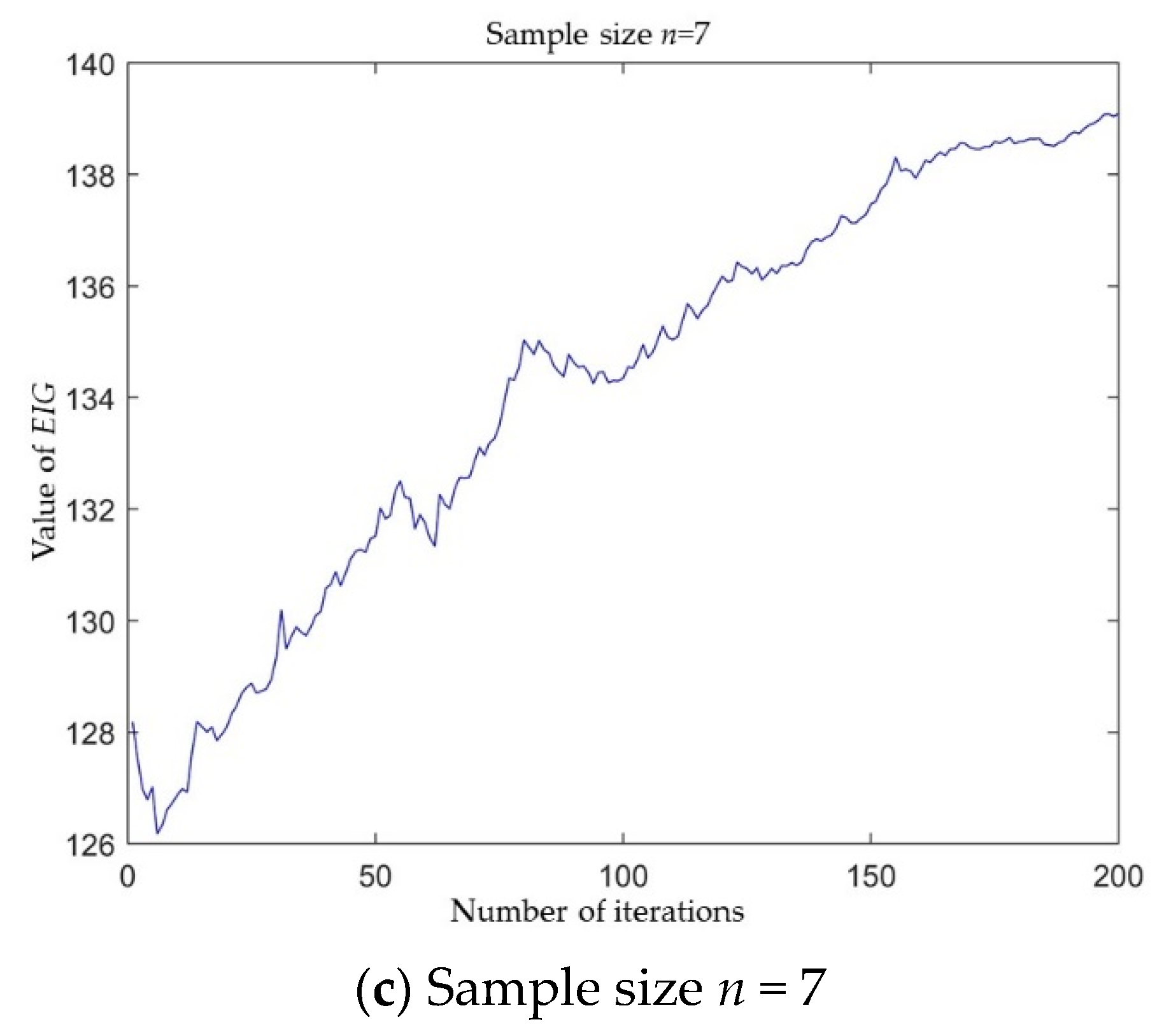Taking into account the cost of the test and the number of model parameters in the established motorized spindle accelerated model, the number of stress levels L in the test is chosen to be 7. The alternative solutions with different sample numbers are solved by genetic algorithm, the iterative process is shown in Figure 6, and the optimal solutions are shown in

Table 7. The optimal test plan of pre-test optimization (n = 5, n = 6).

n = 5		n = 6
$\mathit{m}$	(39, 38, 37, 36, 35, 33, 32)	$\mathit{m}$	(29, 28, 27, 26, 25, 23, 22)
${\mathit{S}}_1$	(30, 69, 153, 217, 304, 461, 500)	${\mathit{S}}_1$	(30, 72, 169, 213, 305, 463, 500)
${\mathit{S}}_2$	(3000, 3520, 4330, 4950, 5710, 6190, 7500)	${\mathit{S}}_2$	(3000, 3510, 4340, 4930, 5720, 6210, 7500)
${\mathit{S}}_3$	(2.10, 3.13, 3.90, 4.69, 5.43, 6.44, 7.00)	${\mathit{S}}_3$	(2.10, 3.16, 3.91, 4.69, 5.46, 6.47, 7.00)
EIG	205.5740	EIG	174.4615

and

Table 8. The optimal test plan of pre-test optimization(n = 7).

n = 7
$\mathit{m}$	(19, 18, 17, 16, 15, 13, 12)
${\mathit{S}}_1$	(30, 73, 172, 217, 308, 466, 500)
${\mathit{S}}_2$	(3000, 3540, 4340, 4970, 5760, 6200, 7500)
${\mathit{S}}_3$	(2.10, 3.17, 3.88, 4.71, 5.47, 6.48, 7.00)
EIG	139.0895

.

From the comparison of the optimal solutions in Table 6 and Table 7, it can be concluded that the smaller the number of samples, the larger the value of EIG for the same test cost. This is because as the number of samples decreases, the cost required for the test samples decreases, allowing more test costs to be spent on the implementation of the test. Conducting the test over a long period of time and collecting more degradation data of the tested motorized spindle, allows the obtaining of a stable posterior distribution of the model parameters. Moreover, the stress levels of the three optimal plans all fluctuate within the same range, indicating that the stress levels in the table are the sensitive stress levels for the accelerated degradation test of the spindle under this objective function, i.e., the optimal test stress levels for this model of the motorized spindle. Although the values of each stress level of the three optimal plans fluctuate in the same range, the values of the low sample size stress levels are all slightly lower than the values of the high sample size stress levels. That is because fewer resources are used to implement the test in the high sample size solution, and the high-stress level values can obtain the degradation information of the motorized spindle faster and thus obtain larger objective function values. The reason for the lower stress values in the low sample size optimal plan is, the closer to the normal stress level of the motorized spindle, the smaller the fluctuation of the a posteriori distribution of the obtained model parameters or even reaches stability, thus making the objective function reach its theoretical maximum.

Based on the above analysis, it is concluded that under the condition that the cost constraint is the main constraint, the sample size of the test should be minimized and the test time should be maximized to obtain a more accurate posterior distribution of the model parameters. Therefore, the optimal test plan with n = 5 in Table 6 is chosen as the initial plan of the test, and the values of each stress level and the EIG at this stress level of this plan are shown in

Table 9. EIG obtained for each stress level in the n = 5 optimal test plan.

Number of Stress Levels	The Value of Stress	Inspections	EIG
1	(30 N, 3000 rpm, 2.10 kW)	39	19.8843
2	(69 N, 3520 rpm, 3.13 kW)	38	21.7920
3	(153 N, 4330 rpm, 3.90 kW)	37	24.5134
4	(217 N, 4950 rpm, 4.69 kW)	36	28.0621
5	(304 N, 5710 rpm, 5.43 kW)	35	32.2650
6	(461 N, 6190 rpm, 6.44 kW)	33	35.4401
7	(500 N, 7500 rpm, 7.5 kW)	32	43.6171
		Total EIG	205.5740

.

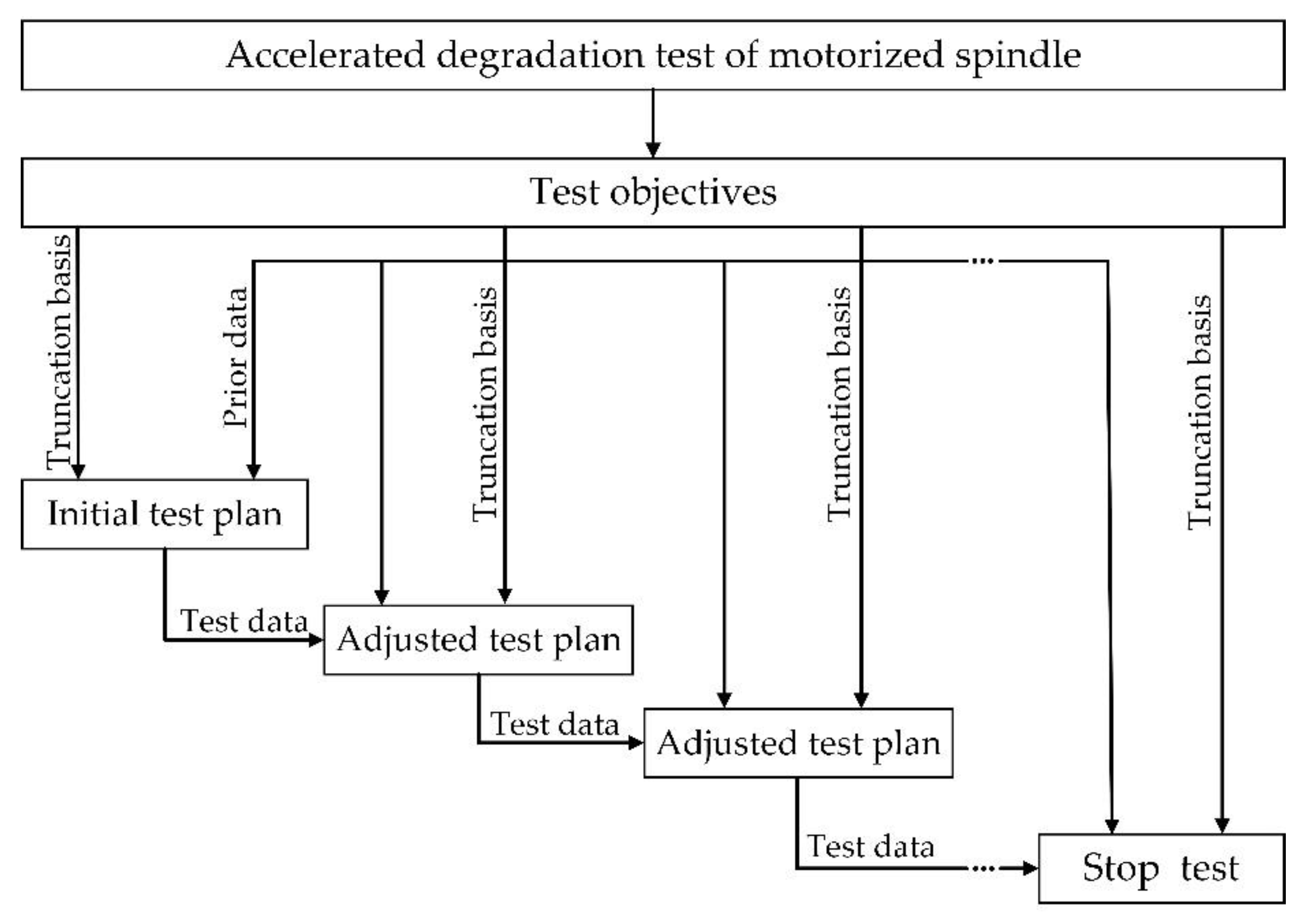
6.2. In-Test Optimization

According to the test plan obtained from pre-test optimization and the Optimization process of the test in Section 5, the test was performed on the tested motor spindle at the highest stress level S_i7, and the test equipment is shown in Figure 5. The posterior distribution of the parameters was calculated based on the obtained performance degradation increment data $\Delta y_7$. The updated probability density function of the posterior distribution of the model parameters with the number of inspections was obtained, as shown in Figure 7.

From Figure 7, it can be obtained that there is a certain deviation between the prior distribution probability density functions of the model parameters based on the prior data of different models of machining center motorized spindles and the tested motorized spindles. In addition, the posterior probability density function of each model parameter generally has the phenomenon of peak shift and variance increase of the distribution graph with the increase in the number of inspections. This is because the posterior distribution probability density function of each model parameter obtained by solving at m₇ = 8 has a certain chance due to the small amount of data, and usually has a certain distance between the true value of the parameter. As the number of tests increases (i.e., the amount of data increases), the chance of the probability density function is gradually eliminated, and the probability density function of the posterior distribution of the model parameters is gradually closer to the true value. At the end of this stress level test, IG = 117.3 > EIG = 43.1671, which satisfies the sequential truncation basis, and the next stress level test is carried out.

The posterior distribution probability density function of each model parameter obtained at m₇ = 32 is used as the prior distribution probability density of each model parameter at stress level l = 6. The process of updating the posterior distribution of each model parameter with the increment data $\Delta y_6$ of performance degradation is shown in Figure 8.

At the end of the test for stress level l = 6, IG = 101.248 > EIG = 35.4401, which satisfies the sequential truncation basis. It can also be seen from Figure 8 that the shifting of the probability density function is weakened compared with the previous stress level. Nevertheless, the posterior distribution probability density function of each model parameter still has large variations, some of which are the shifting of the mean value of the model parameter and some of which are the fluctuations of the variance. This indicates that there are still deviations between the posterior distribution probability density of each model parameter and the true value at this stage, and the chance of the probability density function has not been completely eliminated, so it is necessary to continue the test.

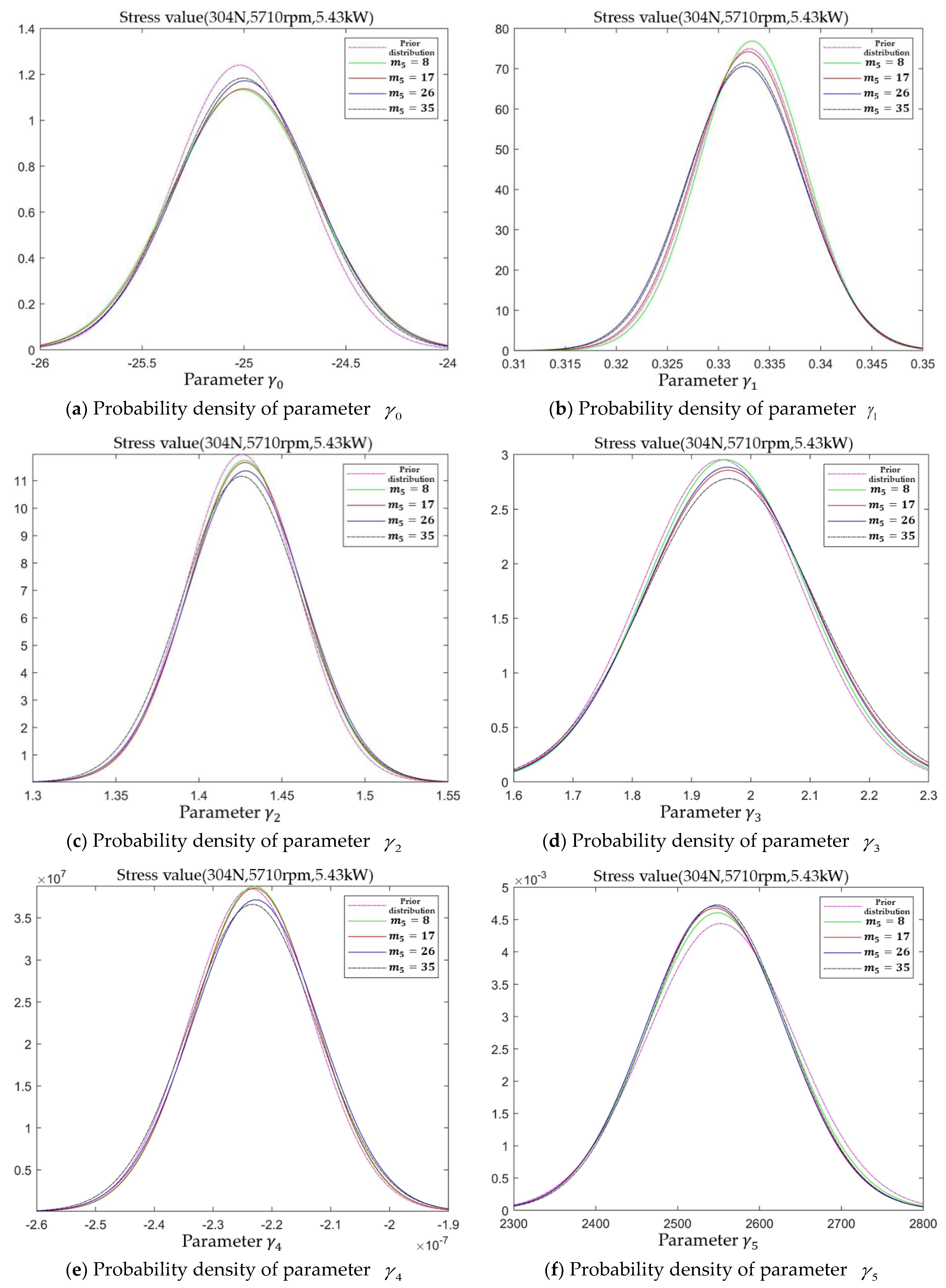
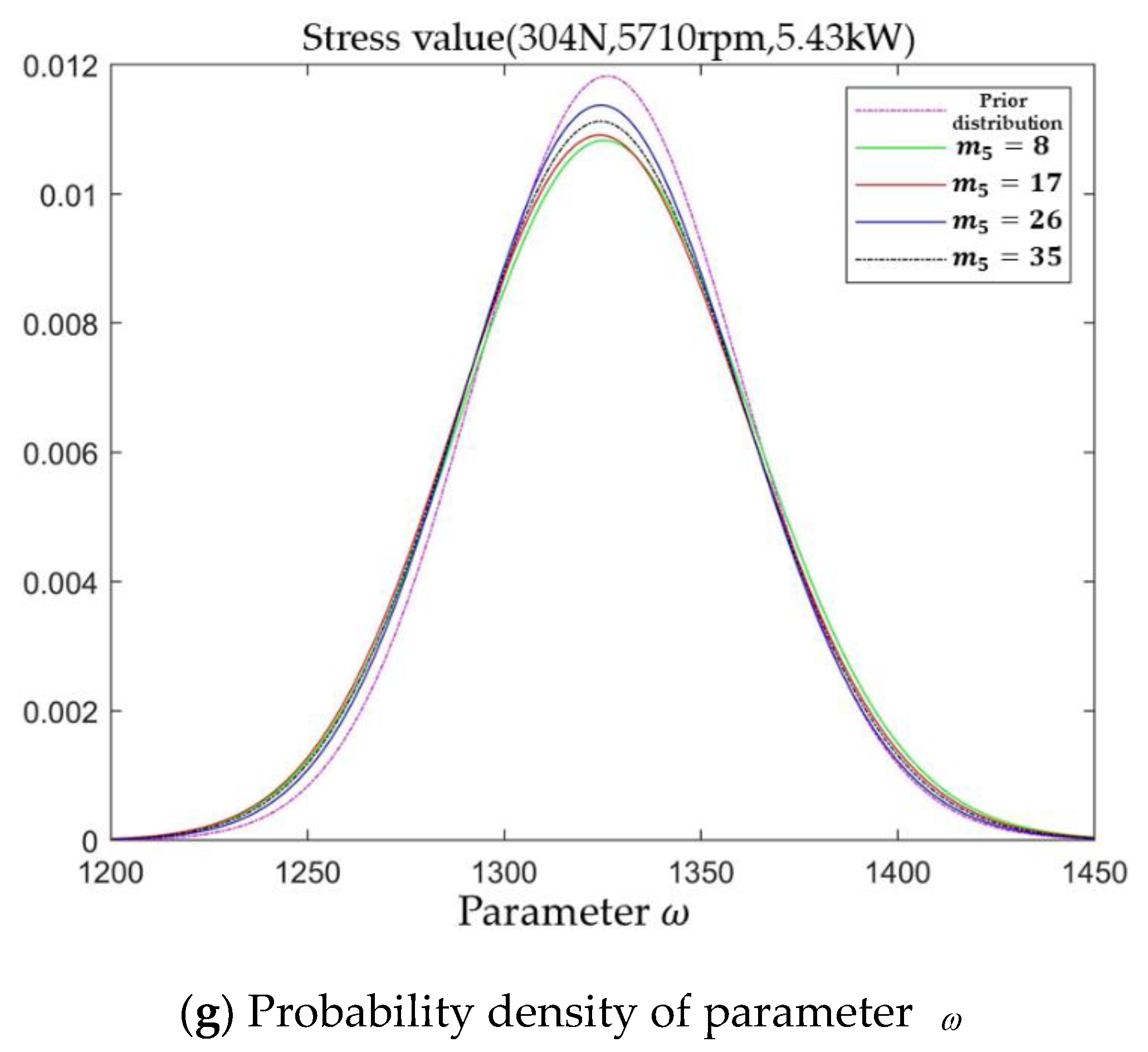
According to the selected test protocol, the test was conducted at stress level l = 5, and the posterior distribution probability density of each model parameter was calculated based on the performance degradation increment data $\Delta y_5$. The updated posterior distribution probability density of each model parameter at stress level l = 5 is shown in Figure 9.

Compared with the probability density function plots of the posterior distribution of model parameters at the first two stress levels, the shifting of the probability density function of the posterior distribution of each model parameter in Figure 9 is basically eliminated, and the fluctuations are mainly the up and down fluctuations of the function images, i.e., the changes of the variance of the posterior distribution. It indicates that the mean value of the posterior distribution has been close to the true value of the model parameters, but it is necessary to continue the test because the function graph is not stable. When the stress level l = 5 ends, IG = 87.661 > EIG = 32.2650, which satisfies the sequential truncation basis for the next stress level, the test of stress level l = 4 is carried out according to the selected test plan. In addition, the variation of the probability density of the posterior distribution of each model parameter with the performance degradation increment data $\Delta y_4$ under this stress level is shown in Figure 10.

At the end of this stress level, IG = 71.918 > EIG = 28.0621, which satisfies the sequential truncation basis, and there are only minor fluctuations in the mean and variance of the posterior distribution probability density functions of the model parameters in Figure 10. This indicates that the posterior distribution of each model parameter is close to the true value of the model parameters; especially the probability density function of the prior distribution of parameter ${\gamma }_0$ at this stress level basically coincides with the probability density function of the posterior distribution. However, because the accelerated model needs to be extrapolated to assess the reliability of the spindle at the normal stress level when evaluating the reliability of the spindle, some of the evaluation accuracy is lost. Therefore, although the fluctuation of the posterior distribution probability density of each model parameter is small at this time, the fluctuation of the posterior distribution probability density function needs to be completely eliminated in order to ensure the evaluation accuracy at the normal stress level, so the test at the next stress level is also required. 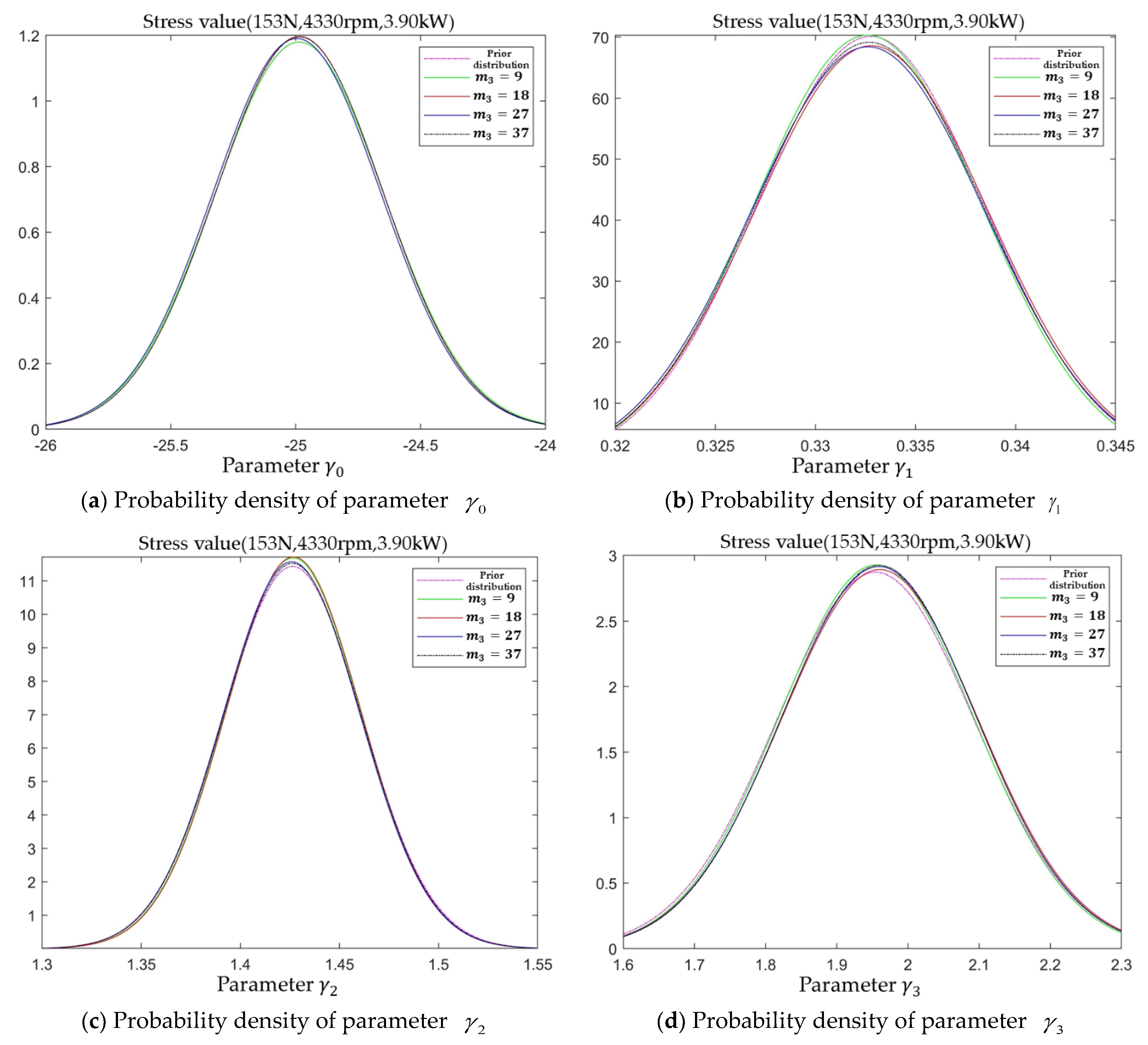According to the selected test plan, the test of stress level l = 3 was conducted, and the posterior distribution of each model parameter is shown in Figure 11.

Compared with Figure 10, the posterior distribution probability density functions of the model parameters in Figure 11 only have small fluctuations in the variance, especially the posterior distribution probability densities obtained for parameters ${\gamma }_0$ and ${\gamma }_4$ at each number of inspections at this stress level almost overlap. Although the variances of the posterior distributions of parameters ${\gamma }_1$, ${\gamma }_5$ and $\omega$ still have more obvious variations, the mean values have not changed significantly. Moreover, the value of IG obtained in the test is 437.589, which is already larger than the EIG = 205.5740 of the test plan. In addition, if the test efficiency is maximized, termination of the test can be considered according to the sequential design method. However, at this time, the distribution of the model parameters, for the first time, appears to stabilize, and in order to eliminate the chance of the test and thus ensure the scientific nature of the study, the next level of the test is conducted to verify it. At the end of this stress level, IG = 59.462 > EIG = 24.5134, which satisfies the sequential truncation basis for the next stress level. 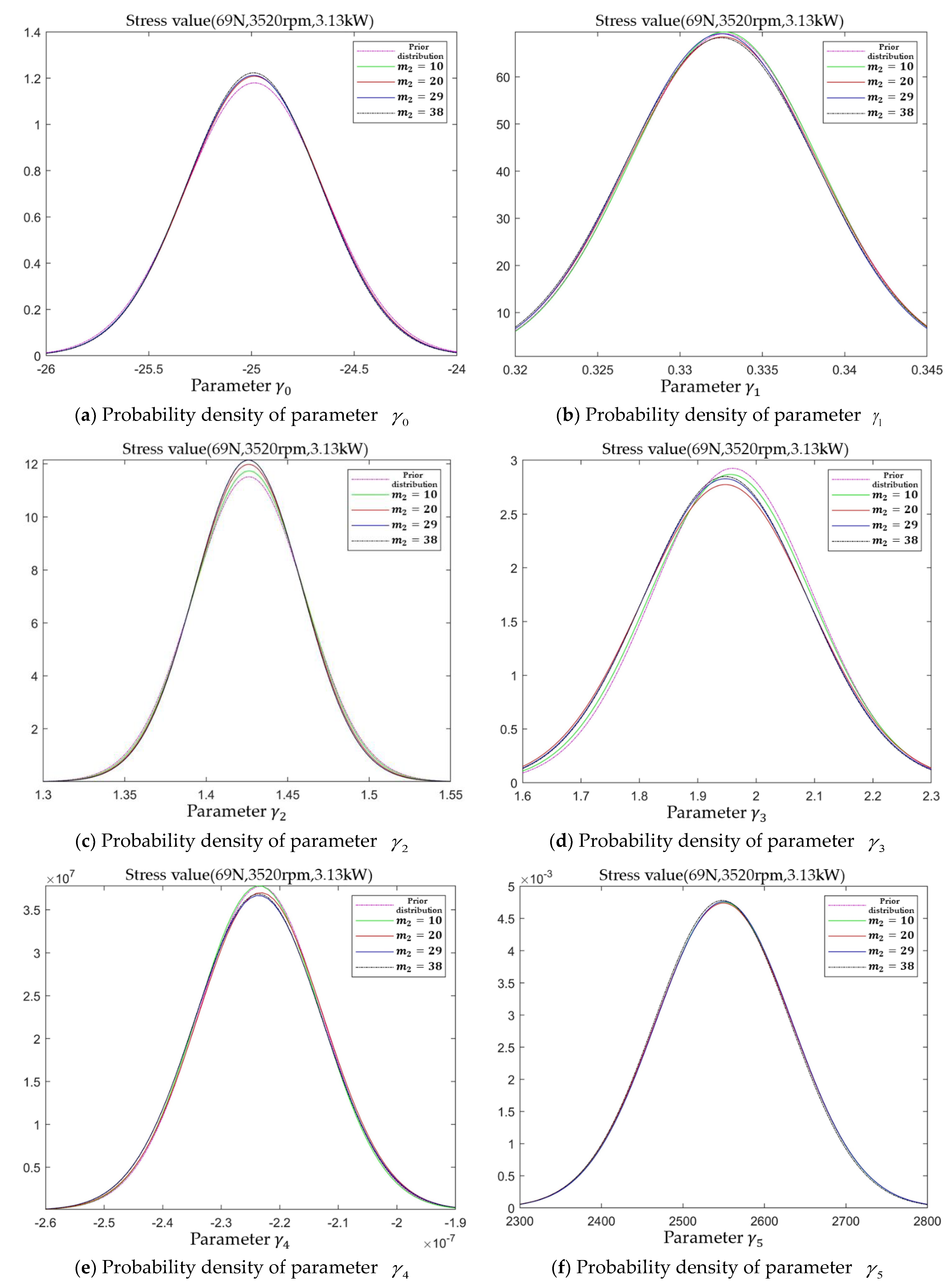According to the selected test plan, the test for stress level l = 2 was conducted, and the procedure is shown in Figure 12.

In Figure 12 there is a significant change between the posterior distribution probability density functions of parameters ${\gamma }_0$, ${\gamma }_2$, ${\gamma }_3$ and ${\gamma }_4$ the prior probability density functions, where ${\gamma }_0$, ${\gamma }_2$ and ${\gamma }_4$ are variance fluctuations and ${\gamma }_3$ is the mean shift. In particular, the posterior distribution of parameter ${\gamma }_0$ at the previous two stress levels has converged to a steady state, but the variance of the experimental parameter ${\gamma }_0$ at this stress level again appears to fluctuate significantly. The above changes in the posterior probability density functions of the parameters indicate that after incorporating the incremental degradation data of the motorized spindle under this stress level, the steady state of the probability density function of each model parameter distribution after the end of the previous stress level is “breaks”. According to the analysis, the changes in the posterior distribution of ${\gamma }_0$, ${\gamma }_2$ and ${\gamma }_4$ are because the randomness of the motorized spindle under this stress level is different from the previous stress level. The change of ${\gamma }_3$ is because the value reaches the false true value at the previous stress level, and continues to approach the true value under this stress level. The change of parameters ${\gamma }_0$, ${\gamma }_2$, ${\gamma }_3$ and ${\gamma }_4$ prove the necessity of continuing the test. However, as the number of inspections at this stress level increases, the change in the probability density function of the posterior distribution of the model parameters gradually decreases. This indicates that with the incorporation of the degradation increment data at this stress level, the posterior distribution of the model parameters at the performed stress level has converged to the true value, i.e., the model can be used to evaluate the reliability of the spindle within the performed stress level. However, there is a certain span between this stress level and the normal stress level. 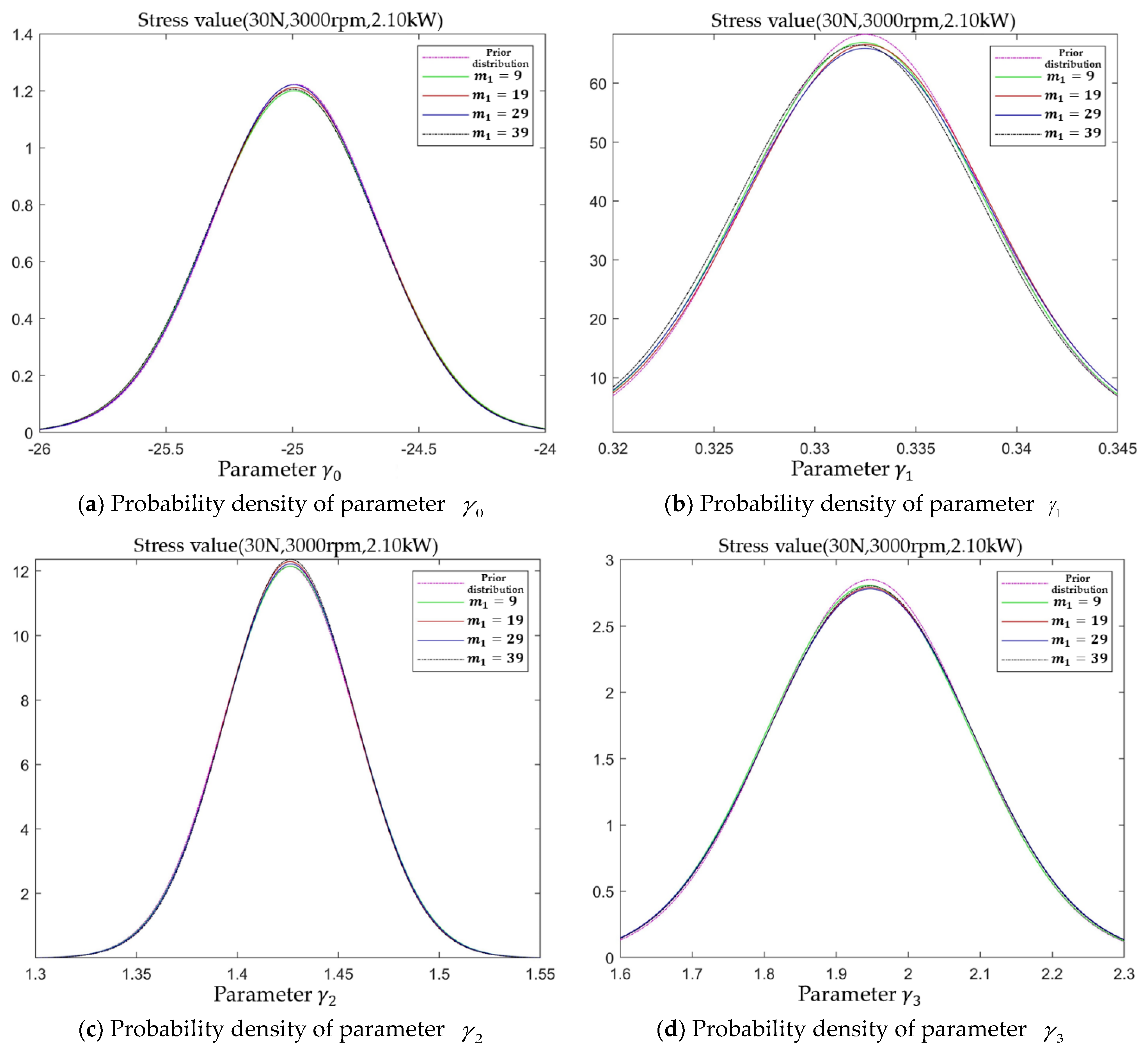In order to avoid the recurrence of this phenomenon after incorporating the data at the normal stress level, and to ensure the extrapolation accuracy of the model at the normal stress level, a test at the normal stress level (l = 1) is required. According to the test plan, the test of normal stress level (l = 1) is implemented, and the probability density of the posterior distribution of each model parameter is shown in Figure 13.

According to Figure 13, it can be seen that the posterior distribution probability density of the model parameters also appears to fluctuate after incorporating the degradation increment data at normal levels. However, compared with Figure 12, the fluctuations have diminished and there are basically no more fluctuations in the model parameters after incorporating some normal stress level data. It can also be concluded from Figure 13 that the fluctuations of model parameters in Figure 13 are mainly variance fluctuations. This fluctuation is mainly caused by the degradation randomness of samples of different motorized spindles at this stress level. In addition, according to the nature of sequential design, the test can be stopped after 19 data tests (m₁ = 19), and although the IG < EIG at this time, the posterior distribution has not changed significantly. In addition, according to the complete test process of the stress level l = 1, the posterior distribution of the model parameters in the subsequent test has tended to the steady state (as shown in

Table 10. The posterior distribution of each model parameter at stress level l = 1.

		${\gamma }_0$	${\gamma }_1$	${\gamma }_2$	${\gamma }_3$	${\gamma }_4$	${\gamma }_5$	$\mathit{\sigma }$
m1 = 9	${\mu }_{\gamma }$	−24.9932	0.3325	1.4263	1.9448	−2.2386 × 10−7	2549.04	$a_{\sigma }$: 1374.23
	${\sigma }_{\gamma }$	0.33246	0.0058	0.0329	0.1421	1.0858 × 10−8	83.4086	$b_{\sigma }$: 0.9618
m1 = 19	${\mu }_{\gamma }$	−24.9923	0.3324	1.4261	1.9472	−2.2376 × 10−7	2549.61	$a_{\sigma }$: 1412.52
	${\sigma }_{\gamma }$	0.3292	0.0060	0.0325	0.1429	1.0915 × 10−8	85.2801	$b_{\sigma }$: 0.9361
m1 = 29	${\mu }_{\gamma }$	−24.9936	0.3326	1.4263	1.9471	−2.2378 × 10−7	2549.59	$a_{\sigma }$: 1431.98
	${\sigma }_{\gamma }$	0.3268	0.0060	0.0326	0.1434	1.0928 × 10−8	84.9894	$b_{\sigma }$: 0.9238
m1 = 39	${\mu }_{\gamma }$	−24.9967	0.3322	1.4263	1.9472	−2.2396 × 10−7	2548.15	$a_{\sigma }$: 1432.45
	${\sigma }_{\gamma }$	0.3309	0.0060	0.0323	0.1423	1.0931 × 10−8	83.8724	$b_{\sigma }$: 0.9233

). So the probability density function of the posterior distribution of each model parameter at m₁ = 19 satisfies the second basis of the sequential truncation basis, and the end of the test can be stopped.

The complete test process was compiled as shown in

Table 11. The complete process of motorized spindle ADT.

		Initial Selection of Test Plan	Sequential Design Test Plan	Actual Test Plan
Stress level (l)	1	(30 N, 3000 rpm, 2.10 kW)	(30 N, 3000 rpm, 2.10 kW)	(30 N, 3000 rpm, 2.10 kW)
	2	(69 N, 3520 rpm, 3.13 kW)	(69 N, 3520 rpm, 3.13 kW)	(69 N, 3520 rpm, 3.13 kW)
	3	(153 N, 4330 rpm, 3.90 kW)	(153 N, 4330 rpm, 3.90 kW)	(153 N, 4330 rpm, 3.90 kW)
	4	(217 N, 4950 rpm, 4.69 kW)	(217 N, 4950 rpm, 4.69 kW)	(217 N, 4950 rpm, 4.69 kW)
	5	(304 N, 5710 rpm, 5.43 kW)	(304 N, 5710 rpm, 5.43 kW)	(304 N, 5710 rpm, 5.43 kW)
	6	(461 N, 6190 rpm, 6.44 kW)	(461 N, 6190 rpm, 6.44 kW)	(461 N, 6190 rpm, 6.44 kW)
	7	(500 N, 7500 rpm, 7.5 kW)	(500 N, 7500 rpm, 7.5 kW)	(500 N, 7500 rpm, 7.5 kW)
Inspections (mi)	1	39	39	39
	2	38	38	38
	3	37	37	37
	4	36	36	36
	5	35	35 (Test can be terminated)	35
	6	33	33 (If the test continues)	33
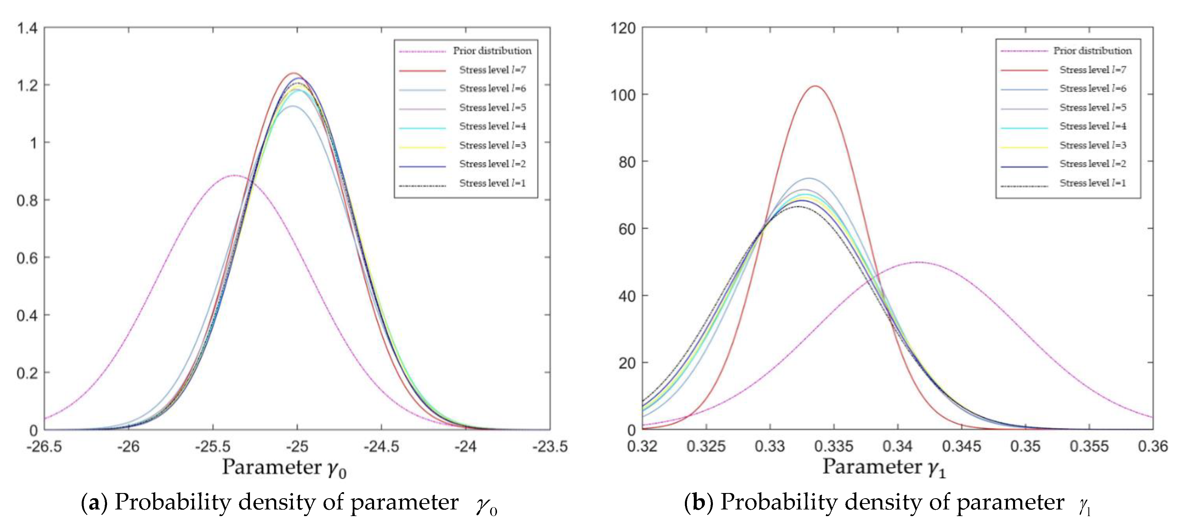
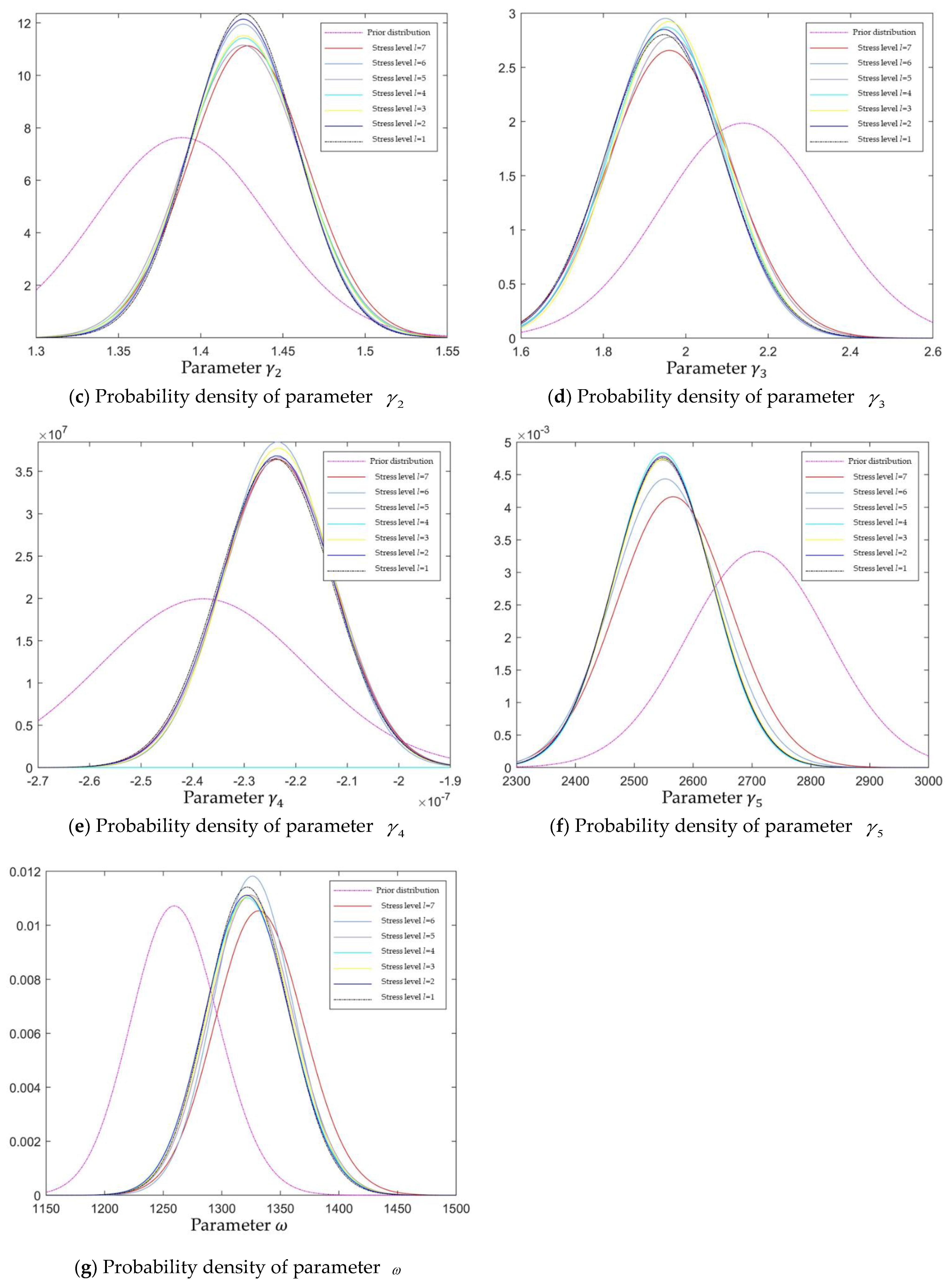
	7	32	19	32

, and the posterior distribution of each model parameter of the motorized spindle was shown in Equation (42), and its update process at each stress level was summarized as shown in Figure 14.

$$\begin{array}{c}{\gamma }_0~N\left(-24.9967,{\left(0.3309\right)}^2\right)\\ {\gamma }_1~N\left(0.3322,{\left(0.0060\right)}^2\right)\\ {\gamma }_2~N\left(1.4263,{\left(0.03227\right)}^2\right)\\ \begin{array}{c}{\gamma }_3~N\left(1.9472,{\left(0.1424\right)}^2\right)\\ {\gamma }_4~N\left(-2.2396\times {10}^{-7},{\left(1.0932\times {10}^{-8}\right)}^2\right)\\ \begin{array}{c}{\gamma }_5~N\left(2548.15,{83.8724}^2\right)\\ 1/{\sigma }^2=\omega ~Ga(1432.45,0.923321)\end{array}\end{array}\end{array}.$$

(42)

As can be seen in Figure 14, there is a large span between the posterior distribution probability density and the prior distribution probability density for each model parameter when the prior information is poor. There is also a large span between the posterior distribution probability density for the first stress level (l = 7) and the posterior distribution probability density for the seventh stress level (l = 1). This span illustrates that there is a large deviation between the prior parameter values and the true values in the presence of poor prior information, which in turn justifies the need for the research conducted in this article.

It can also be seen from Figure 14 that compared with the span of the prior distribution and the posterior distribution, the span of the posterior distribution and the posterior distribution after the first stress in the test is significantly reduced, which proves the necessity of dynamic adjustment of the test plan in the test when the prior information is poor. In addition, the probability density of the posterior distribution of the model parameters at the first few stress levels (l $\ge$ 4) is dominated by the shift of the mean, i.e., towards the true value of the model. The probability densities of the posterior distributions of the model parameters at the latter stress levels are dominated by the variance shifts, i.e., the distributions are adjusted according to the differences in the samples. In addition, the posterior probability densities of most of the model parameters have leveled off after the fifth stress level (l = 3). Especially after the seventh stress level has been carried out for a period of time, the posterior distribution probability densities of each model parameter almost do not change anymore, indicating that the parameters have reached the true values of the samples, which in turn proves the availability of the method in optimizing the test plan.

6.3. Validation of the Proposed Method Validity

The problem with the optimal design of a motorized spindle ADT plan when the prior information is poor is that deviations between the prior model parameter values and the true values make it impossible to carry out an accurate optimal design of the test plan using traditional optimization design methods. This is because in the traditional optimization design method, the model parameters are determined values, and the test scheme is optimized based on the determined model parameters. When the prior information is poor, there is a large deviation between the obtained model parameter value and the true value, so there is a large deviation between the obtained “optimal” plan and the real optimal plan. This leads to unsatisfactory test results and a waste of test resources. The optimal design method proposed in this article takes maximizing information entropy as the optimization objective and aims to correct the deviations between the prior model parameters and the true values of the model parameters, so in order to verify the validity of the method, the accuracy of the tested model also needs to be verified.

However, since the performance degradation data obtained in the example is accelerated degradation data, the accuracy of the model can only be verified based on this data. The data obtained at different stress levels are substituted into the degradation model, and if

$$\frac{\Delta y_{ljk}-{\mu }_l\times \Delta t^{\partial }}{\sqrt{{\sigma }^2\Delta t^{\partial }}}~N\left(0,1\right)$$

(43)

holds, then the model established is accurate, where ${\mu }_l$, ${\sigma }^2$ can be found by taking the value of each stress level in the test and the mean value of each model parameter in Equation (42).

To facilitate the statistics of the test results, the conversion results of the data at each stress level are represented in the form of a Quantile-Quantile plot, as shown in Figure 15.

It can be seen in Figure 15 that the distributions of degradation data and model permutation results under each stress level basically obey the standard normal distribution, and the models under each stress level can obey the standard normal distribution well. This indicates that the acceleration model has high extrapolation accuracy, i.e., the model parameters obtained have high accuracy, which in turn proves the validity of the proposed optimal design method in solving the problem of optimal design of the three-stress ADT plan for motorized spindles when the prior information is poor.

7. Conclusions

This article addresses the problem that the current optimization design method cannot accurately optimize the design of the three-stress ADT plan for motorized spindles when the prior information is poor and carries out the corresponding optimal design method research. The specific research work is as follows:

• In order to solve the problem of the deviation between the prior parameter value and the “true value” of the three-stress accelerated degradation model of the motorized spindle when the prior information is poor, a random variable is used to replace the traditional determined value. Based on the conjugate prior distribution and kernel function, the specific expression of the prior distribution of each model parameter of the three-stress accelerated degradation model of the motorized spindle with stress coupling term is determined.
• To eliminate the deviation between the prior model parameters and the “true value” caused by the poor prior information to the maximum extent, the corresponding optimization design method is proposed based on the information entropy, and the constraint conditions and the value space of the test plan are determined.
• Incorporating sequential design into the optimal design method to realize the “dynamic” adjustment of the test plan in the test, so as to eliminate the optimization deviation caused by the poor prior information.
• Introducing a genetic algorithm to improve the speed of solving the pre-test optimization, and sorting out the proposed optimization method to give a complete optimization step and optimization process.
• The optimized design of the three-stress ADT plan with poor prior information was carried out for a model of motorized spindle made in China, to verify the usability of the method. In addition, the accuracy of the tested model was checked to verify the validity of the method.

References

1. Yang, Z.; Chen, C.; Chen, F.; Li, G. Progress in the Research of Reliability Technology of Machine Tools. J. Mech. Eng. 2013, 49, 130–139. [Google Scholar] [CrossRef]
2. Zhang, Y.; Zhang, C.; Yan, J.; Yang, C.; Liu, Z. Rapid construction method of equipment model for discrete manufacturing digital twin workshop system. Robot. Comput. Integr. Manuf. 2022, 75, 102309–102327. [Google Scholar] [CrossRef]
3. Zhang, Z.; Cheng, Q.; Qi, B.; Tao, Z. A general approach for the machining quality evaluation of S-shaped specimen based on POS-SQP algorithm and Monte Carlo method. J. Manuf. Syst. 2021, 60, 553–568. [Google Scholar] [CrossRef]
4. Li, G.; Zhong, Y.; Chen, C.; Jin, T.; Liu, Y. Reliability allocation method based on linguistic neutrosophic numbers weight Muirhead mean operator. Expert Syst. Appl. 2022, 193, 116504. [Google Scholar] [CrossRef]
5. Jin, T.; Yan, C.; Chen, C.; Yang, Z.; Tian, H.; Guo, J. New domain adaptation method in shallow and deep layers of the CNN for bearing fault diagnosis under different working conditions. Int. J. Adv. Manuf. Technol. 2021, 1–13. [Google Scholar] [CrossRef]
6. Cheng, Q.; Qi, B.; Liu, Z.; Zhang, C.; Xue, D. An accuracy degradation analysis of ball screw mechanism considering time-varying motion and loading working conditions. Mech. Mach. Theory 2019, 134, 1–23. [Google Scholar] [CrossRef]
7. Zhao, H.; Yang, Z.; Chen, C.; Tian, H.; Chen, L.; Ying, J.; Jia, X. Development of Reliability Test System Based on Working Principle and Fault Analysis of Motorized Spindle. In Proceedings of the 2018 3rd International Conference on System Reliability and Safety (ICSRS), Barcelona, Spain, 23–25 November 2018. [Google Scholar]
8. Nelson, W. Analysis of Performance-Degradation Data from Accelerated Tests. IEEE Trans. Reliab. 1981, R-30, 149–155. [Google Scholar] [CrossRef]
9. Meeker, W.Q.; Escobar, L.A.; Lu, C.J. Accelerated Degradation Tests: Modeling and Analysis. Technometrics 1998, 40, 89–99. [Google Scholar] [CrossRef]
10. Park, J.; Yum, B. Optimal design of Accelerated Degradation Tests for estimating mean lifetime at the use condition. Eng. Optim. 1997, 28, 199–230. [Google Scholar] [CrossRef]
11. Amini, M.; Shemehsavar, S.; Pan, Z. Optimal Design for Step-Stress Accelerated Test with Random Discrete Stress Elevating Times Based on Gamma Degradation Process. Qual. Reliab. Eng. Int. 2016, 32, 2391–2402. [Google Scholar] [CrossRef]
12. Wang, H.; Zhao, Y.; Ma, X.; Wang, H. Optimal design of constant-stress accelerated degradation tests using the M-optimality criterion. Reliab. Eng. Syst. Saf. 2017, 164, 45–54. [Google Scholar] [CrossRef]
13. Hu, C.; Lee, M.; Tang, J. Optimum step-stress accelerated degradation test for Wiener degradation process under constraints. Eur. J. Oper. Res. 2015, 241, 412–421. [Google Scholar] [CrossRef]
14. Tseng, S.; Balakrishnan, N.; Tsai, C. Optimal Step-Stress Accelerated Degradation Test Plan for Gamma Degradation Processes. IEEE Trans. Reliab. 2009, 58, 611–618. [Google Scholar] [CrossRef]
15. Lim, H. Optimum accelerated degradation tests for the gamma degradation process case under the constraint of total cost. Entropy 2015, 17, 2556–2572. [Google Scholar] [CrossRef] [Green Version]
16. Tsai, T.-R.; Sung, W.-Y.; Lio, Y.L.; Chang, S.I.; Lu, J.-C. Optimal Two-Variable Accelerated Degradation Test Plan for Gamma Degradation Processes. IEEE Trans. Reliab. 2016, 65, 459–468. [Google Scholar] [CrossRef]
17. Duan, F.; Wang, G. Optimal step-stress accelerated degradation test plans for inverse Gaussian process based on proportional degradation rate model. J. Stat. Comput. Simul. 2018, 88, 305–328. [Google Scholar] [CrossRef]
18. Chen, Z.; Li, S.; Pan, E. Optimal Constant-Stress Accelerated Degradation Test Plans Using Nonlinear Generalized Wiener Process. Math. Probl. Eng. 2016, 2016, 9283295. [Google Scholar] [CrossRef] [Green Version]
19. Pan, Z.; Sun, Q. Optimal design for step-stress accelerated degradation test with multiple performance characteristics based on gamma processes. Commun. Statistics. Simul. Comput. 2014, 43, 298–314. [Google Scholar] [CrossRef]
20. Limon, S.; Rezaei, E.; Yadav, O.P. Designing an accelerated degradation test plan considering the gamma degradation process with multi-stress factors and interaction effects. Qual. Technol. Quant. Manag. 2019, 17, 544–560. [Google Scholar] [CrossRef]
21. Li, X.; Hu, Y.; Zio, E.; Kang, R. A Bayesian Optimal Design for Accelerated Degradation Testing Based on the Inverse Gaussian Process. IEEE Access 2017, 5, 5690–5701. [Google Scholar] [CrossRef]
22. Li, X.; Hu, Y.; Sun, F.; Kang, R. A Bayesian optimal design for sequential accelerated degradation testing. Entropy 2017, 19, 325. [Google Scholar] [CrossRef] [Green Version]
23. Yu, Y.; Hu, C.; Si, X.; Zhang, J. Modified Bayesian D-Optiality for Accelerated Degradation Test Design With Model Uncertainty. IEEE Access 2019, 7, 42181–42189. [Google Scholar] [CrossRef]
24. Balakrishnan, N.; Qin, C. Nonparametric optimal designs for degradation tests. J. Appl. Stat. 2020, 47, 624–641. [Google Scholar] [CrossRef] [PubMed]
25. Zivkovic, A.; Zeljkovic, M.; Tabaković, S.; Milojević, Z. Mathematical modeling and experimental testing of high-speed spindle behavior. Int. J. Adv. Manuf. Technol. 2015, 77, 1071–1086. [Google Scholar] [CrossRef]
26. Yang, Z.; Li, X.; Chen, C.; Zhao, H.; Yang, D.; Guo, J.; Luo, W. Reliability assessment of the spindle systems with a competing risk model. Proc. Inst. Mech. Engineers. Part O J. Risk Reliab. 2019, 233, 226–234. [Google Scholar] [CrossRef]
27. Li, X. Research on Multiple-Stress Reliability Accelerated Model of Spindle System in Machining Centers. Ph.D. Thesis, University of Jilin, Changchun, China, 2019. [Google Scholar]
28. Bao, J. Reliability Modeling of Motorized Spindle Based on Step-Stress Accelerated Degradation Test with Two Accelerating Stresses. Master’s Thesis, University of Jilin, Changchun, China, 2019. [Google Scholar]
29. Jin, G. Reliability Technology Based on Degradation—Model, Method and Application; National Defense Industry Press: Beijing, China, 2014. [Google Scholar]
30. Cai, Z.; Chen, Y.; Zhang, Z.; Xiang, H. Reliability assessment method of nonlinear step-stress accelerated degradation data. J. Beijing Univ. Aeronaut. Astronaut. 2016, 42, 576–582. [Google Scholar]
31. Han, M. Bayesian Statistics—Application Based on R and Bugs; Tongji University Press: Shanghai, China, 2017. [Google Scholar]
32. Xu, T.; Wang, H.; Zhang, X. Application of EM algorithm to estimate hyper parameters of the random parameters of Wiener process. Xi Tong Gong Cheng Yu Dian Zi Ji Shu 2015, 37, 707–712. [Google Scholar]
33. Dong, C.; Lu, H.; Wang, S. Application of kernel of probability density function in statistical calculation. J. Xinjiang Norm. Univ. (Nat. Sci. Ed.) 2020, 39, 29–33. [Google Scholar]
34. Ntzoufras, I. Bayesian Modeling Using WinBUGS; John Wiley and Sons: New York, NY, USA, 2009. [Google Scholar]
35. Holland, J. Adaptation in Natural and Artificial Systems; MIT Press: Cambridge, MA, USA, 1992. [Google Scholar]
36. Lewis, S.M.; Raftery, A.E. Estimating Bayes Factors via Posterior Simulation with the Laplace-Metropolis Estimator. J. Am. Stat. Assoc. 1997, 92, 648–655. [Google Scholar]
37. Guo, J. Multi-Objective Optimization Design Method of Accelerated Degradation Test for Motorized Spindle with Uncertain Model. Ph.D. Thesis, University of Jilin, Changchun, China, 2021. [Google Scholar]
Figure 1. The performance degradation track of motorized spindle.
Metals 12 01996 g001
Figure 2. Relationship of model parameters.
Metals 12 01996 g002
Figure 3. General flow of sequential design for ADT plan of motorized spindle.
Metals 12 01996 g003
Figure 4. Optimization process of three-stress ADT plan of motorized spindle with poor prior information.
Metals 12 01996 g004
Figure 5. The Actual test equipment of motorized spindle.
Metals 12 01996 g005
Figure 6. Iterative process of the optimal solution of pre-test optimization.
Metals 12 01996 g006aMetals 12 01996 g006b
Figure 7. The update process of probability density of each model parameter with the test (l = 7).
Metals 12 01996 g007aMetals 12 01996 g007b
Figure 8. The update process of probability density of each model parameter with the test (l = 6).
Metals 12 01996 g008aMetals 12 01996 g008b
Figure 9. The update process of probability density of each model parameter with the test (l = 5).
Metals 12 01996 g009aMetals 12 01996 g009b
Figure 10. The update process of probability density of each model parameter with the test (l = 4).
Metals 12 01996 g010aMetals 12 01996 g010b
Figure 11. The update process of probability density of each model parameter with the test (l = 3).
Metals 12 01996 g011aMetals 12 01996 g011b
Figure 12. The update process of probability density of each model parameter with the test (l = 2).
Metals 12 01996 g012aMetals 12 01996 g012b
Figure 13. The update process of probability density of each model parameter with the test (l = 1).
Metals 12 01996 g013aMetals 12 01996 g013b
Figure 14. The update process of the posterior distribution of each model parameter.
Metals 12 01996 g014aMetals 12 01996 g014b
Figure 15. The Quantile-Quantile plot of model and standard normal distribution.
Metals 12 01996 g015