Abstract
The present paper provides an accurate solution for finite plane strain bending under tension of a rigid/plastic sheet using a general material model of a strain-hardening viscoplastic material. In particular, no restriction is imposed on the dependence of the yield stress on the equivalent strain and the equivalent strain rate. A special numerical procedure is necessary to solve a non-standard ordinary differential equation resulting from the analytic treatment of the boundary value problem. A numerical example illustrates the general solution assuming that the tensile force vanishes. This numerical solution demonstrates a significant effect of the parameter that controls the loading speed on the bending moment and the through-thickness distribution of stresses.
1. Introduction
Bending is frequently used as a test for determining various material properties. A four-point bend apparatus was used in [1] for getting stress–strain curves in the tension and compression of three materials: beryllium, cast iron, and copper. No significant difference between these curves and the corresponding curves from the conventional uniaxial tension and compression tests was found. Papers [2,3] applied the same method for determining the stress–strain curves for annealed copper and cement-based composites, respectively. The theoretical solution proposed in [1] was modified in [4]. Then, the method was used for determining the stress–strain curves for pure magnesium and S45C steel. Paper [5] studied the elastic/plastic behavior and the failure of CLARE laminates in bending experimentally. An elastic/plastic material model was proposed using these experimental data. Lightweight-aggregate concrete beams were tested in bending to failure in [6]. This work emphasized the location of the neutral axis at failure. Adhesively bonded bending specimens were employed in [7] for determining the bilinear elastic/plastic shear stress–strain behavior of acrylic adhesives. Hybrid sandwich structures were tested in bending in [8] to construct failure mode maps.
Experimental data should be usually supplemented with theoretical solutions for identifying material models. Most semi-analytic solutions have dealt with strain hardening materials [9,10,11,12]. Paper [12] also accounted for plastic anisotropy and tension/compression asymmetry. The representation of strain or work hardening in the strain reversal region has been simplified in these works. Paper [13] developed a semi-analytic method to treat this region without any simplification. This method was combined with various constitutive equations to describe pure bending and bending under tension of wide sheets [14]. Under certain conditions, viscoplastic or strain-hardening viscoplastic constitutive equations are required to analyze bending processes adequately [15,16,17]. Many material models of this type are available in the literature [18,19,20,21,22,23,24]. For identifying constitutive equations, it is desirable to have a theoretical solution for a general material model. The motivation of the present paper is to provide a semi-analytic solution of the same level of complexity as available solutions but for quite a general material model. It is believed that such a solution is useful for identifying constitutive equations. The solution is based on the general method proposed in [13].
The solution found is facilitated by using the equivalent strain instead of the space coordinate as an independent variable. Similar changes of independent variables have been successfully used in several works [25,26,27]. In particular, the process of bending was analyzed in [26]. However, in all these cases, it has been assumed that the yield stress depends on the single kinematic quantity, the equivalent plastic strain. The novelty of the present solution is that the yield stress is an arbitrary function of the equivalent strain and the equivalent strain rate. An important property of the new solution is that process parameters depend on the loading speed. In addition, the solution shows that some assumptions used in simplified formulations are not valid and corresponding numerical results may lead to the misinterpretation of experimental data.
2. Statement of the Problem
What is considered is the process of bending under tension due to large strains under plane strain conditions in the classical formulation proposed in [28], where a model of rigid perfectly plastic material was adopted. A schematic diagram of the process is shown in Figure 1. The cross section of a sheet is rectangular at the initial instant. The initial thickness of the sheet is H. As the deformation proceeds, the initially straight lines and become circular arcs and , respectively. The initially straight lines and remain straight (lines and , respectively). The radii of circular arcs and are denoted as and , respectively. A Cartesian coordinate system is introduced. Its x-axis coincides with the axis of symmetry of the process. Its origin coincides with the intersection of the outer radius of the sheet and the axis of symmetry. Due to symmetry, it is sufficient to consider the domain . The orientation of line relative to the x-axis is . The actual distribution of stresses over is replaced with the bending moment M and the tensile force F. Both are per unit length. The surface is traction-free. Equilibrium requires that the tensile force is compensated with pressure over the surface . It is assumed that this pressure is uniformly distributed.
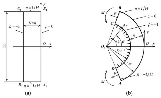
Figure 1.
Schematic diagram of the bending process: (a) initial configuration and (b) intermediate and final configurations.
Then,
The constitutive equations include an isotropic pressure-independent yield criterion (i.e., the linear invariant of the stress tensor does not affect plastic yielding) and its associated flow rule. The elastic portion of the strain tensor is neglected. The present paper assumes that the tensile yield stress is a function of the equivalent strain, , and the equivalent strain rate, , obtained by fitting any experimental data. Then, the plane-strain yield criterion can be represented as
Here and are the principal stresses, is a reference stress, and is an arbitrary function of its arguments. The associated flow rule is equivalent to the equation of incompressibility and the condition that the stress and strain rate tensors are coaxial. In the case under consideration, the equivalent strain rate is determined as
where and are the principal strain rates. The equivalent plastic strain is given by
here denotes the convected derivative.
3. Kinematics
The approach for solving plane-strain bending problems proposed in [13] consists of two major steps. The first step describes the kinematics of the process. This step is the same for all isotropic incompressible materials. The second step concerns the determination of the stresses, bending moment, and tensile force. This step depends on the constitutive equations chosen. The present section outlines the basic relations from the first step derived in [13]. These relations are necessary for the second step.
Let be the Lagrangian coordinate system satisfying the conditions and at the initial instant. Then, on and on throughout the process of deformation (Figure 1). The transformation equations between the and coordinate systems are
Here a is a time-like variable and s is a function of a. At the initial instant, . The function should be found from the solution. This function must satisfy the condition
at . The coordinate lines of the Lagrangian coordinate system coincide with principal strain rate trajectories [13]. Then, the coordinate lines of the Lagrangian coordinate system coincide with principal stress trajectories for the coaxial models. Therefore, the contour of the cross-section is free of shear stresses throughout the process of deformation.
It is convenient to introduce a cylindrical coordinate system by the transformation equations:
Equations (5) and (7) combine to give
Therefore, the radial, , and circumferential, , stresses are the principal stresses. In what follows, it is assumed that and . Accordingly, and . Here is the radial strain rate and is the circumferential strain rate. It follows from (8) that
It is straightforward to find the principal strain rates using (5). In particular,
Equations (3) and (10) combine to give
The equivalent strain rate vanishes at the neutral line. Therefore, it follows from (11) that the coordinate of the neutral line is
The neutral line moves through the material as the deformation proceeds. It is known that it moves towards CD in the case of strain-hardening materials. Assume that it is true in the case of the constitutive equations under consideration. Specific calculations below will verify this assumption. The initial condition for Equation (4) is
at . Let be the value of at . It is necessary to consider three regions for determining the equivalent strain. These regions are: (Region 1), (Region 2), and (Region 3). In Region 1, throughout the process of deformation. Therefore, one can substitute (11) into (4) and immediately integrate the resulting equation using (13) and (6) to get
In Region 3, throughout the process of deformation. Therefore, one can substitute (11) into (4) and immediately integrate the resulting equation using (13) and (6) to get
In Region 2, instantly. However, strain reversal occurs in this region. Consider any curve of Region 2. Let be the value of a at which this curve coincides with the neutral line and is the corresponding value of s. Evidently, both and are functions of . Then, the equivalent strain in Region 2 is given by
4. Stress Solution
The only stress equilibrium equation that is not satisfied automatically in the cylindrical coordinate system is
The yield criterion (2) can be represented as
Here and in what follows, in regions 1 and 2, and in region 3. Equations (17) and (18) combine to give
Using (8), one can replace differentiation with respect to r with differentiation with respect to . As a result,
One can rewrite Equation (11) as
Here , is a characteristic strain rate, and . Equations (14) and (15) can be rewritten as
One can eliminate in (21) using (22). As a result,
Using (22), one can replace differentiation with respect to with differentiation with respect to . Then, Equation (20) becomes
Using (23), one can represent the function as
Equations (24) and (25) combine to give
Since on surface AB, the distribution of the radial stress in region 1 is determined from (26) and (27) as
Here is a dummy variable of integration and denotes the function when in (23). The value of at is determined from (14) as
Then, the radial stress at is found from (28) in the form
Using (9), one can represent (1) as
where . It follows from (26), (31), and (32) that the distribution of the radial stress in region 3 is
Here denotes the function when in (23). The value of at is determined from (12) and (15) as
Then, the radial stress at is found from (33) in the form
In region 2, Equation (20) becomes
Here the function is determined by replacing and in with the right-hand sides of equations (16) and (21), respectively. The radial stress must be continuous at and . Therefore, using (35), one can represent the solution of Equation (36) as
Equations (30) and (37) combine to give
This equation connects a, s, and . Therefore, it can be considered an ordinary differential equation to find s as a function of a. Its solution must satisfy the condition (6).
Once Equation (38) has been solved, the distribution of the radial stress in all three regions is readily determined from (28), (33), and (37). Equations (28) and (33) should be used in conjunction with Equations (14) and (15), respectively. The distribution of the circumferential stress is found from (18). The bending moment is given by
Note that in the case of rigid perfectly plastic material if [28].
5. Numerical Method
It has been noted that Equation (38) is an ordinary differential equation. Several well-established methods are available for solving such equations numerically (see, for example, [29]). However, the form of the differential equation in Equation (38) is non-standard. Therefore, a special numerical method should be developed to solve this equation. The method below is a modification of the method developed in [30] for solving a system of partial differential equations.
Equation (38), together with Equation (6), constitutes the initial value problem. However, a difficulty is that the equation provides no information at the initial instant. In particular, each term of this equation vanishes at a = 0 since εeq = 0 everywhere. It is a consequence of rigid plasticity. Such difficulty does not arise in elastic/plastic solutions (see, for example, [31]). Below, the difficulty noted is resolved by finding the state of stress at the initial instant without using Equation (38) and developing a general iterative procedure.
Assume that and at , and and are known. Let be a small increment of a. Then, , and the value of s at can be approximated as
Here is the value of the derivative at , and its value is unknown. Using (27), (29), (31), (34), and (41), one can express the limits of integration involved in (38) in terms of and known quantities. Thus Equation (38) determines . The procedure above can be repeated for and subsequent values of a.
It remains to find s and at to start the iterative procedure above. The required value of s is given by (6). The initial cross-section of the sheet is shown in Figure 1a. The through-thickness stress vanishes at this instant. The equivalent strain vanishes everywhere. Equation (21) becomes
Here is the value of the derivative at . Equations (2) and (42) combine to give
The tensile force at the initial instant is determined as
Substituting (43) into (44) gives
This equation determines . In particular, if (pure bending). The dimensionless bending moment can be found using (40), where should be replaced with .
6. Numerical Example
The numerical results below are for pure bending. Several functions are available in the literature [18,19,20,21,22,23,24]. Since bending of strain-hardening materials, including quantitative results, has been investigated in many papers, the numerical example below emphasizes the effect of loading speed on process parameters.
In most cases, the function is represented as a product of two functions. One of these functions depends on the equivalent strain and the other on the equivalent strain rate. The illustrative example in this section assumes that is the product of Swift’s strain-hardening law and Herschel–Bulkley’s viscoplastic law. Then,
In all calculations, , , and . The characteristic strain rate is involved in the solution only through . In particular, one can rewrite (46) as
The numerical solution has been found using the procedure described in the previous section. It demonstrates the effect of on the through-thickness distribution of stresses and the bending moment. Figure 2 and Figure 3 depict the through-thickness distributions of the radial and circumferential stresses, respectively, at several process stages identified by the inner radius of the sheet. These distributions correspond to . In these figures,
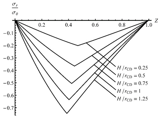
Figure 2.
Through-thickness distribution of the radial stress at γ = 0.1 and several process stages.
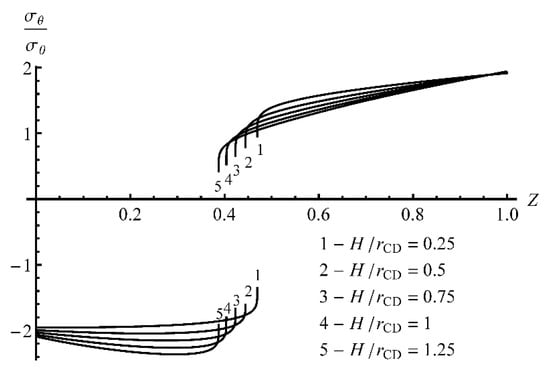
Figure 3.
Through-thickness distribution of the circumferential stress at γ = 0.1 and several process stages.
Thus corresponds to the inner radius of the sheet and to its outer radius. Using (8) and (9), one transforms Equation (48) to
At the final stage of the process, the inner radius of the sheet is rather small (smaller than the initial thickness of the sheet). Figure 4 and Figure 5 show the same distributions at . The circumferential stress is discontinuous at the neutral line. Figure 3 and Figure 5 show that the neutral line moves to the inner surface of the sheet as the deformation proceeds. Thus the assumption made in Section 3 has been confirmed. The magnitude of the radial stress is quite high near the neutral line, except at the very beginning of the process (see Table 1). Therefore, the assumption used in simplified solutions [32,33] that the radial stress is negligible is not valid. The rightmost points of the curves in Figure 2, Figure 3, Figure 4 and Figure 5 correspond to . Therefore, it is seen from these figures that the change in the thickness is negligible.
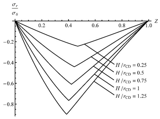
Figure 4.
Through-thickness distribution of the radial stress at γ = 1 and several process stages.
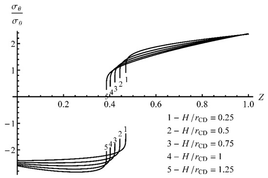
Figure 5.
Through-thickness distribution of the circumferential stress at γ = 1 and several process stages.

Table 1.
Radial stress at the neutral line.
Figure 6 demonstrates the effect of on the dimensionless bending moment. The broken line corresponds to the rate-independent material model (i.e., the material obeys Swift’s strain-hardening law). The bending moment increases as increases, which is in agreement with physical expectations. The increase in the bending moment is sharper for smaller values of . It is worthy of note that the bending moment is nearly constant for a given value of .
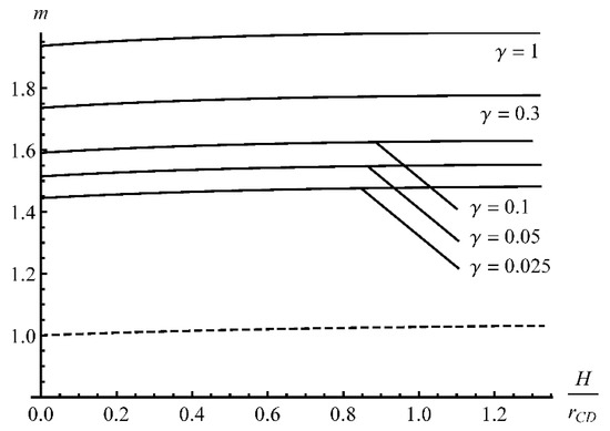
Figure 6.
Variation of the dimensionless bending moment as the deformation proceeds at several values of γ. The broken line corresponds to the rate-independent material.
7. Conclusions
An accurate rigid plastic solution for a general strain-hardening viscoplastic material model has been found. The solution describes the plane strain process of bending under tension due to large strains. The elastic portion of the strain tensor has been neglected. However, the effect of elasticity on the accuracy of solutions is negligible except at the beginning of the process [34].
The numerical solution reduces to an ordinary differential equation in a non-standard form. A special numerical procedure is required to solve this equation. The procedure is described in Section 5. It is used to determine the stress field and the bending moment in the pure bending of a sheet made of a material obeying Equation (46). This numerical solution is presented and discussed in detail in Section 6.
The solution presented may be considered a starting point for designing experiments to identify constitutive equations. It is advantageous in this respect that the general solution is not restricted to a specific function or even a class of functions but is valid for an arbitrary dependence of the yield stress on the equivalent strain and the equivalent strain rate.
The solution can be used as a benchmark problem for verifying numerical codes. This necessary step applies to different constitutive equations, including equations used in metal forming applications [35,36,37].
Author Contributions
Conceptualization and writing, S.A.; formal analysis and writing E.L. All authors have read and agreed to the published version of the manuscript.
Funding
This research was made possible by grant 20-69-46070 from the Russian Science Foundation.
Institutional Review Board Statement
Not applicable.
Informed Consent Statement
Not applicable.
Data Availability Statement
Not applicable.
Conflicts of Interest
The authors declare no conflict of interest.
References
- Mayville, R.A.; Finnie, I. Uniaxial stress-strain curves from a bending test. Exp. Mech. 1982, 22, 197–201. [Google Scholar] [CrossRef]
- Oldroyd, P.W.J. Tension-compression stress-strain curves from bending tests. J. Strain Anal. 1971, 6, 286–292. [Google Scholar] [CrossRef]
- Laws, V. Derivation of the tensile stress-strain curve from bending data. J. Mater. Sci. 1981, 16, 1299–1304. [Google Scholar] [CrossRef]
- Kato, H.; Tottori, Y.; Sasaki, K. Four-point bending test of determining stress-strain curves asymmetric between tension and compression. Exp. Mech. 2014, 54, 489–492. [Google Scholar] [CrossRef] [Green Version]
- Solyaev, Y.; Lurie, S.; Prokudin, O.; Antipov, V.; Rabinskiy, L.; Serebrennikova, N.; Dobryanskiy, V. Elasto-plastic behavior and failure of thick GLARE laminates under bending loading. Compos. Part B Eng. 2020, 200, 108302. [Google Scholar] [CrossRef]
- Bernardo, L.; Nepomuceno, M.; Pinto, H. Neutral axis depth versus ductility and plastic rotation capacity on bending in lightweight-aggregate concrete beams. Materials 2019, 12, 3479. [Google Scholar] [CrossRef] [Green Version]
- Alves, M.M.; Abreu, L.M.; Pereira, A.B.; De Morais, A.B. Determination of bilinear elastic-plastic models for an acrylic adhesive using the adhesively bonded 3-point bending specimen. J. Adhes. 2021, 97, 553–568. [Google Scholar] [CrossRef]
- Rupp, P.; Elsner, P.; Weidenmann, K.A. Failure mode maps for four-point-bending of hybrid sandwich structures with carbon fiber reinforced plastic face sheets and aluminum foam cores manufactured by a polyurethane spraying process. J. Sandw. Struct. Mater. 2019, 21, 2654–2679. [Google Scholar] [CrossRef]
- Dadras, P.; Majlessi, S.A. Plastic bending of work hardening materials. ASME. J. Eng. Ind. 1982, 104, 224–230. [Google Scholar] [CrossRef]
- Dadras, P. Plane strain elastic–plastic bending of a strain-hardening curved beam. Int. J. Mech. Sci. 2001, 43, 39–56. [Google Scholar] [CrossRef]
- Heller, B.; Kleiner, M. Semi-analytical process modelling and simulation of air bending. J. Strain Anal. Eng. Des. 2006, 41, 57–80. [Google Scholar] [CrossRef]
- Ahn, K. Plastic bending of sheet metal with tension/compression asymmetry. Int. J. Solids Struct. 2020, 204–205, 65–80. [Google Scholar] [CrossRef]
- Alexandrov, S.; Kim, J.-H.; Chung, K.; Kang, T.-J. An alternative approach to analysis of plane-strain pure bending at large strains. J. Strain Anal. Eng. Des. 2006, 41, 397–410. [Google Scholar] [CrossRef]
- Alexandrov, S.; Lyamina, E.; Hwang, Y.-M. Plastic bending at large strain: A review. Processes 2021, 9, 406. [Google Scholar] [CrossRef]
- Parsa, M.; Rad, M.; Shahhosseini, M.R.; Shahhosseini, M. Simulation of windscreen bending using viscoplastic formulation. J. Mater. Process. Technol. 2005, 170, 298–303. [Google Scholar] [CrossRef]
- Alvarez González, C.M.; Okabe, T. Application of multiplicative viscoplastic model to deformation analysis of creep bending test of structural steel. J. Struct. Constr. Eng. 2018, 83, 1343–1351. [Google Scholar] [CrossRef]
- Saito, N.; Fukahori, M.; Minote, T.; Funakawa, Y.; Hisano, D.; Hamasaki, H.; Yoshida, F. Elasto-viscoplastic behavior of 980 MPa nano-precipitation strengthened steel sheet at elevated temperatures and springback in warm bending. Int. J. Mech. Sci. 2018, 146–147, 571–582. [Google Scholar] [CrossRef]
- Perrone, N. A mathematically tractable model of strain-hardening, rate-sensitive plastic flow. ASME. J. Appl. Mech. 1966, 33, 210–211. [Google Scholar] [CrossRef]
- Shang, H.; Wu, P.; Lou, Y. Strain hardening of AA5182-O considering strain rate and temperature effect. In Forming the Future. The Minerals, Metals & Materials Series; Daehn, G., Cao, J., Kinsey, B., Tekkaya, E., Vivek, A., Yoshida, Y., Eds.; Springer: Cham, Switzerland, 2021; pp. 657–665. [Google Scholar] [CrossRef]
- De Angelis, F.; Cancellara, D.; Grassia, L.; D’Amore, A. The influence of loading rates on hardening effects in elasto/viscoplastic strain-hardening materials. Mech. Time-Depend. Mater. 2018, 22, 533–551. [Google Scholar] [CrossRef]
- Lomakin, E.; Fedulov, B.; Fedorenko, A. Strain rate influence on hardening and damage characteristics of composite materials. Acta Mech. 2021, 232, 1875–1887. [Google Scholar] [CrossRef]
- Li, Z.; Wang, J.; Yang, H.; Liu, J.; Ji, C. A modified Johnson–Cook constitutive model for characterizing the hardening behavior of typical magnesium alloys under tension at different strain rates: Experiment and simulation. J. Mater. Eng. Perform. 2020, 29, 8319–8330. [Google Scholar] [CrossRef]
- Heydarian, M.; Shafiei, E.; Ostovan, F. A phenomenological model utilizing Voce’s strain-hardening model describing high strain rate behavior of alloy 800H during hot working. J. Strain Anal. Eng. Des. 2020, 55, 271–276. [Google Scholar] [CrossRef]
- Ghazani, M.S.; Eghbali, B. Strain hardening behavior, strain rate sensitivity and hot deformation maps of AISI 321 austenitic stainless steel. Int. J. Miner. Metall. Mater. 2021. [Google Scholar] [CrossRef]
- Durban, D.; Baruch, M. Analysis of an elasto-plastic thick walled sphere loaded by internal and external pressure. Int. J. Non-Linear Mech. 1977, 12, 9–21. [Google Scholar] [CrossRef]
- Alexandrov, S.; Hwang, Y.-M. Plane strain bending with isotropic strain hardening at large strains. Trans. ASME J. Appl. Mech. 2010, 77, 064502. [Google Scholar] [CrossRef]
- Alexandrov, S.; Pirumov, A.; Jeng, Y.-R. Expansion/contraction of a spherical elastic/plastic shell revisited. Cont. Mech. Therm. 2015, 27, 483–494. [Google Scholar] [CrossRef]
- Hill, R. The Mathematical Theory of Plasticity; Clarendon Press: Oxford, UK, 1950. [Google Scholar]
- Atkinson, K.; Han, W.; Stewart, D. Numerical Solution of Ordinary Differential Equations; John Wiley & Sons: Hoboken, NJ, USA, 2009. [Google Scholar]
- Alexandrov, S.; Gelin, J.-C. Plane strain pure bending of sheets with damage evolution at large strains. Int. J. Solids Struct. 2011, 48, 1637–1643. [Google Scholar] [CrossRef] [Green Version]
- Alexandrov, S.; Manabe, K.; Furushima, T. A general analytic solution for plane strain bending under tension for strain-hardening material at large strains. Arch. Appl. Mech. 2011, 81, 1935–1952. [Google Scholar] [CrossRef]
- Yuen, W.Y.D. A generalised solution for the prediction of springback in laminated strip. J. Mater. Process. Technol. 1996, 61, 254–264. [Google Scholar] [CrossRef]
- Kagzi, S.A.; Gandhi, A.H.; Dave, H.K.; Raval, H.K. An analytical model for bending and springback of bimetallic sheets. Mech. Adv. Mater. Struct. 2016, 23, 80–88. [Google Scholar] [CrossRef]
- Alexandrov, S.; Lyamina, E.; Hwang, Y.-M. Finite pure plane strain bending of inhomogeneous anisotropic sheets. Symmetry 2021, 13, 145. [Google Scholar] [CrossRef]
- Roberts, S.M.; Hall, F.; Van Bael, A.; Hartley, P.; Pillinger, I.; Sturgess, E.N.; Van Houtte, P.; Aernoudt, E. Benchmark tests for 3-D, elasto-plastic, finite-element codes for the modelling of metal forming processes. J. Mater. Process. Technol. 1992, 34, 61–68. [Google Scholar] [CrossRef]
- Abali, B.E.; Reich, F.A. Verification of deforming polarized structure computation by using a closed-form solution. Contin. Mech. Thermodyn. 2020, 32, 693–708. [Google Scholar] [CrossRef]
- Yang, H.; Timofeev, D.; Abali, B.E.; Li, B.; Muller, W.H. Verification of strain gradient elasticity computation by analytical solutions. ZAMM 2021, 101, e202100023. [Google Scholar] [CrossRef]
Publisher’s Note: MDPI stays neutral with regard to jurisdictional claims in published maps and institutional affiliations. |
© 2022 by the authors. Licensee MDPI, Basel, Switzerland. This article is an open access article distributed under the terms and conditions of the Creative Commons Attribution (CC BY) license (https://creativecommons.org/licenses/by/4.0/).