A Novel Machine-Learning-Based Procedure to Determine the Surface Finish Quality of Titanium Alloy Parts Obtained by Heat Assisted Single Point Incremental Forming

Abstract

Single point incremental forming (SPIF) is a cheap and flexible sheet metal forming process for rapid manufacturing of complex geometries. Additionally, it is important for engineers to measure the surface finish of work pieces to assess their quality and performance. In this paper, a predictive model based on machine learning and computer vision was developed to estimate arithmetic mean surface roughness (Ra) and maximum peak to valley height (Rz) of Ti6Al4V parts obtained by SPIF. An image database was prepared to train different classification algorithms in accordance with a supervised learning approach. A speeded up robust feature (SURF) detector was used to obtain visual vocabulary so that the classifiers are able to group the photographs into classes. The experimental results indicated that the proposed predictive method shows great potential to determine the surface quality, as classifiers based on a support vector machine with a polynomial kernel are suitable for this purpose.

1. Introduction

Market requirements, along with the development of the industrial sector, have led to parts being demanded under restrictive specifications. As a result, surface finish has emerged as a key aspect of many products in which this feature is critical.

Single Point Incremental Forming (SPIF) is a rapid manufacturing technique based on the localized plastic deformation of sheet metal by a hemispherical tool [1]. For that, the sheet is fixed to a rigid frame and the deformation is produced, moving the tool according to an helicoidal path and establishing a pitch value to feed the operation. The method has generated considerable research interest because it overcomes some of the disadvantages of conventional forming. The SPIF process is characterized by its ability to economically develop complex geometries by means of reduced tooling costs if short series or prototypes are being produced, notably in biomedical and aeronautical applications [2,3,4]. The process has been applied to commercial copper, some aluminum alloys, and high formability mild steel. Some application with stainless steel AISI 304 has been also reported [5]. With regard to titanium alloys, research is mainly recent, and it supposes that their application has the most potential. However, titanium alloys, particularly Ti6Al4V, have a poor formability at room temperature which classifies them into the hard-to-form materials group. Thus, it is necessary to heat the sheet to carry out the SPIF process, also called heat assistant SPIF or HA-SPIF. Consequently, substantial efforts have been undertaken in recent years to develop heating methods. Götmann et al. [6] worked on the process of dynamic heating by laser, previously proposed by Duflou et al. [7]. Fan et al. [8] developed a heating procedure based on Joule heating by electric power from the tool to the sheet, which has also been adopted by other authors [9]. Ambrogio et al. [10] designed an external heating system using electric bands. Similar systems have been applied by Naranjo et al. [11] and Ortiz et al. [12]. There have been attempts to improve formability using the local heating generated between the tool friction on the sheet metal when it rotates at high speed [13]. This procedure is known as Stir-SPIF. Finally, some methods mixing friction and external sources of heat can be found in literature [14].

Despite the improvement reached by HA-SPIF methods, the obtained surface finishes are low quality. There have been some efforts to improve the surface finish after the SPIF process trying to reduce the friction tool sheet without lubricant [15] or considering the effect of lubricant on the process [16], but with a few exceptions, the research has been focused on only room temperature and not on titanium alloys.

Additionally, the influence of surface quality on the operability of the parts promotes the constant development of measurement methods. In recent decades, this sector has undergone successive updates in order to obtain a reliable, precise, and flexible technique to measure surface finish.

Contact profilometry is one of the most common methods in surface finish measuring despite having several drawbacks. Its use is often restricted to controlled environments because it is highly sensitive to vibrations and the stylus can cause flaws on the surface of the part. These limitations, together with its slowness, render it an unsuitable method for measuring online surface roughness.

Optical non-contact methods arose as a necessary alternative to overcome these drawbacks. Of these techniques, the procedure developed by Moreas et al. [17] should be mentioned. In this work, an optical microscope was built to capture images and topography was studied using the principle of triangulation. From another perspective, in the research conducted by Lehmann [18], interferometry techniques were employed in order to analyze the statistical properties of speckle patterns to obtain significant surface roughness parameters. However, non-destructive optical methods do not always achieve the level of precision provided by contact profilometry and samples must be adapted for each of them. Particularly, optical microscopes equipped with profilometer function could be appropriate with higher accuracy in the measurement of surface roughness, but the measuring field is too small and the sample must be split from the part. The dominant key issues for future research include systematic process planning, tool-path optimization, compensating unwanted deformations, advanced feature recognition techniques, forming reliable and robust communication interfaces, flexible hardware, adaptive control methods, the ability to form newer materials and a wider range of materials, complex shapes with ease and accuracy, and removing barriers on sizes of components.

Artificial intelligence has become very popular in this field because machine learning techniques are capable of developing predictive models that provide better results than analytical ones. Machine learning algorithms have been shown to help reduce the number of experiments required to establish a correlation between surface roughness and manufacturing parameters with great effectiveness.

Thus, machine learning has been used to analyze the influence on surface finish of the parameters involved in the manufacturing process. The aim is to optimize the process by maximizing the number of suitable parts. In this regard, Abd et al. [19] developed a gradient boosting regression tree (GBRT) algorithm to establish a correlation between the operating parameters and surface quality of aluminum/stainless steel (Al/SUS) bimetal sheets obtained by SPIF. This research used artificial intelligence to expand on bimetal sheets the results obtained by Echrif and Hrairi [20] in single-layer sheets of aluminum alloy AA105-0.

The use of machine learning algorithms for measuring surface quality allows the limitations of traditional methods to be overcome. Models built with this methodology have proven to be accurate and able to adapt production speeds. In this context, the work by Mulay et al. [21] focuses on a feedforward backpropagation network that was implemented to predict the average surface roughness and maximum forming wall-angle of parts of aluminum alloy AA5052-H32 obtained by SPIF. This experiment showed that artificial neural networks are a promising tool with great economic benefits, greater predictability, and low simulation time.

The work developed by Abu-Mahfouz et al. [22] considered a classifier based on a support vector machine to obtain surface roughness from vibration signals collected during the milling of aluminum parts. In addition, this work analyzed the effect of different types of kernels and sets of features on the performance of the model. Their proposed classification model was trained with 32 different combinations of the milling process conditions and managed to predict the surface roughness with an accuracy of 81.25%.

Furthermore, the research by Koblar et al. [23] developed a computer vision method based on machine learning for surface roughness measurement. Decision trees were used to solve classification and regression problems on a database formed by 300 commutator images taken in 8-bit grayscale. This experiment offers new possibilities for evaluating surface quality and develops a suitable method for applying online roughness measurement without contact. However, the nature of the work calls for the use of a broad set of samples with respect to inputs based on manufacturing parameters.

The research conducted by Kurra et al. [24] developed predictive models for the average and the maximum surface roughness measurement (Ra and Rz) after the SPIF process based on different techniques: Artificial Neural Networks, Support Vector Regression, and Genetic Programming. In the training of these models, the effect of tool diameter, step depth, wall angle, feed rate, and lubricant type were taken into consideration as process variables. Each parameter was varied over three levels to study different combinations of manufacturing parameters and achieve a uniform distribution of roughness values. Roughness was thus analyzed from a technical viewpoint, so this method requires knowing in advance the conditions in which the parts were manufactured.

Other works, such as that by Lin et al. [25], have used deep neural networks, long short-term memory networks, and one-dimensional convolutional neural networks for the prediction of arithmetic mean roughness from vibration signals obtained in the milling process of S45C steel parts. Li et al. [26] compared the results from different classifiers to predict the surface roughness of polylactic acid intake flanges obtained by 3D printing. In both studies, Fast Fourier Transform (FFT) was used to extract the features’ raw data and different techniques were evaluated to build an accurate predictive model.

The literature review showed that several studies have developed predictive models for surface quality measuring of work pieces produced by different processes. However, no research has focused on the application of machine learning techniques to predict the surface quality from images of pieces created by incremental forming, among other reasons, because of the large number of samples required for the model training and the amount of time needed to acquire the features. To fill this gap, the aim of this work was to develop a new methodology for the evaluation of surface quality using photographs of twenty-one parts formed by SPIF as inputs in machine learning classifiers. This procedure would allow the surface finish to be determined without the need to previously know the manufacturing conditions. In this way, surface quality could be studied in real time during the production process.

The remainder of the paper is organized as follows. Section 2 contains an introduction on machine learning and explains the experimental setup in detail. Section 3 describes the data preparation and the training of predictive models. Section 4 presents an evaluation of the predictive model performance and discusses the experimental results. Finally, Section 5 provides findings and future directions.

2. Materials and Methods

Machine learning is a subset of artificial intelligence, the purpose of which is to train computers so they are able to learn automatically through experience. Algorithms are used to build a predictive mathematical model capable of generalizing a behavior without being explicitly programmed [27,28]. In this way, the computer acquires the ability to recognize patterns in sample data to predict future unseen data. Machine learning methods are usually categorized in accordance with their strategy, data processing, and the objective of the application.

Firstly, in the supervised learning approach training, data are composed of a set of previous analyzed examples whose outputs are known. Using these observations as inputs, the computer can learn general rules and establish a correlation to obtain an inferred function, being able to determine the output for new data. On the other hand, human intervention is not required in unsupervised learning algorithms. In this case, a predictive model is trained with unseen data that have not been studied. As a result, it must identify a pattern without previous knowledge. Thirdly, reinforcement learning is a method built on the interaction with its environment. Feedback is used to develop the model through rewards and punishments. Systems learn by analyzing the behavior of their surroundings in response to their actions to maximize positive signals.

This paper focuses on supervised learning to build a predictive model to obtain arithmetic mean roughness from the images of a piece manufactured by incremental forming; as a result, labelled and categorized photographs are used as training data. To this end, the developed model must be capable of extracting characteristics from examples and achieving a relationship between image features and outputs in order to apply this knowledge on new unobserved data.

Having set the objective, the working methodology can be divided into two separate stages: the first phase, aimed at measuring the parts and creating a database that would be used to train machine learning algorithms; the second stage concerning the development and the validation of the classification model.

Experimental Details of Measuring Process of Workpieces

We measured 0.8 mm thick Ti6Al4V alloy parts obtained by a heat-assisted SPIF process to determine the 3D average and maximum roughness parameters (Sa and Sz). The corresponding waviness parameters (Wa and Wz) were also considered. The pieces consisted of cone trunks with a variable wall angle; the angle of the cones was continuously increasing with the forming depth in order to determine the SPIF formability of the alloy. WC and steel tools with a spherical tip of 10 and 12 mm were used and the processing temperature was within the range of 25–400 °C [11]. Parts were created in a Deckel Maho machining center, model DMC 835V (DMG MORI, CO., LTD.,Bielefeld, Germany). A hole frame was built to fasten the sheet. An electric suitably isolated mini-oven was specifically designed and fitted inside the support. The forming strategy adopted was a helical path with a pitch of 0.5 mm per revolution, a feed rate of 600 mm per min, and without any lubrication. To minimize any friction between tool and sheet, a counter-rotation speed of the tool was set at 30 rpm.

The sheet in virgin state always is covered by a TiO₂ layer that was not removed by a previous surface treatment, as it is usual in the SPIF for guaranteeing a same initial surface state in all tests.

The parts were specially selected to have a heterogeneous collection of surface finish values (

Table 1. Single point incremental forming parameters and surface finish values. The value of wall angle in brackets corresponds to the maximum angle formed. (Initial sheet thickness = 0.8 mm, pitch = 0.5 mm/rev, feed rate = 600 mm/min).

Test	Temp. (°C)	Angle (°)	Max. Depth (mm)	Tool (Diameter (mm)/ Material)	Ra (µm)	Rz (µm)	Wa (µm)	Wz (µm)
1	Room	Var (30)	11.4	12/WC	0.976	18.2	0.539	5.73
2	200	Var (40)	17.1	12/WC	0.561	9.87	0.356	2.48
3	300	Var (40)	18.1	12/WC	0.534	15.5	0.344	2.82
4	400	Var (50)	21.1	12/WC	0.521	9.95	0.544	3.43
5	400	40	18	12/WC	1.1	34.8	1.39	17.9
6	400	45	18	12/WC	1.37	34.5	1.65	22.6
7	Room	Var (30)	11.3	12/STEEL	0.704	13.7	0.716	6.22
8	200	Var (40)	15.6	12/STEEL	0.828	14.4	0.801	6.93
9	300	Var (40)	17.5	12/STEEL	1.11	26.9	1.39	13.1
10	400	Var (50)	20.2	12/STEEL	1.05	25.3	0.93	8.03
11	Room	Var (30)	12.5	10/WC	0.862	18.4	0.541	5
12	Room	Var (30)	12.5	10/WC	1.18	20.9	0.841	5.08
13	200	Var (40)	16.3	10/WC	0.913	20.1	0.583	5.53
14	200	Var (40)	16.3	10/WC	0.808	20.3	0.68	5.8
15	300	Var (50)	21.5	10/WC	0.775	37	0.569	5.31
16	400	Var (50)	22.1	10/WC	1.61	26.3	2.09	10.8
17	200	Var (40)	16.4	12/STEEL	1.35	31.9	0.946	7.08
18	300	Var (40)	19.1	12/STEEL	0.816	11.6	0.708	6.05
19	300	Var (40)	19.8	12/STEEL	1.45	30.7	0.699	8.66
20	Room	Var (30)	11.8	12/STEEL	1.48	23.4	0.668	5.48

). The roughness and waviness values reported in Table 1 correspond to measurements taken in intermediate positions of the rolling direction.

A profilometer Form Talysurf 50 and the Talymap software (6.0, Taylor Hobson Ltd., LE4 9JQ, Leicester, UK) were used to measure the roughness and to process the measuring data. An inductive gauge with a 2 µm radius was employed. A block diagram of the measurement procedure is shown in Figure 1. Measurements were carried out on surfaces of 5 mm × 2 mm along three different directions with respect to the rolling direction of the sheet, that is, 0°, 45°, and 90°. The measuring instrument provided an initial profile with some differences to the real surface because of the limitations of the contact profilometry, that is, the gauge radius. From the measured surface, the primary surface is obtained once its shape (the curvature in this case) is removed. Finally, by using a gaussian filter, the irregularities of the primary profile can be split up in the roughness and waviness profiles.

According to the shape of the parts obtained by the SPIF process, it was considered appropriate to apply a polynomial of degree 7 to remove that shape and obtain the primary surface. Some filters were then studied in order to separate the roughness and waviness surfaces that comprise the primary surface. The Gaussian filter is currently the most widely used filtering tool in three-dimensional models because of its isotropic transmission and lack of phase shift according to the standards ISO 11562 and ASME B46. Nevertheless, the symmetry of the filter may cause problems in the edge treatment, which must be removed. Alternately, the spline filter is based on a matrix algorithm which prevents edge defects and is characterized by fast calculations and complex geometry filtering. Nevertheless, this filter has not been widely used in the measurement of 3D surfaces because of its severe anisotropic characteristics. Finally, the robust Gaussian filter used an iterative statistical method in order to improve the Gaussian filter response. This technique allows for a topographic reconstruction without being affected by accidental surface defects. However, it demands large amounts of computation time. Finally, a Gaussian filter, including an edge treatment, was applied by using the Talymap Gold software from Taylor Hobson (6.0, Taylor Hobson Ltd., Leicester, UK).

As a result of the application of the Gaussian filter, roughness and waviness three-dimensional profiles were obtained. These were then used to gather surface finish parameters to build a database.

Concurrently, an Olympus SZX7 (Olympus Corp., Tokyo, Japan) stereoscopic microscope was used to take photographs of the measured surfaces. The images, with dimensions of approximately 6.2 mm × 6 mm, were labelled in accordance with the direction and the position in which they were photographed. Additionally, every image was distributed in files associated with the part to which it belonged. As an example, Figure 2 shows the images taken from Part 5 in the rolling direction (0°). Although the references of the different areas are represented for a frustum with a variable wall angle, the part depicted in Figure 2 corresponds to a constant wall angle cone.

3. Data Preparation and Model Training

Building a database is highly time consuming, not only to process the collected images, but also to train predictive models with them. For this purpose, it is necessary to previously know the functionality of the model.

Two types of problems can generally be distinguished when a supervised learning approach is used. First, classification questions are intended to categorize unknown data into known discrete ranges named classes, while the aim of regression algorithms is to predict a continuous value.

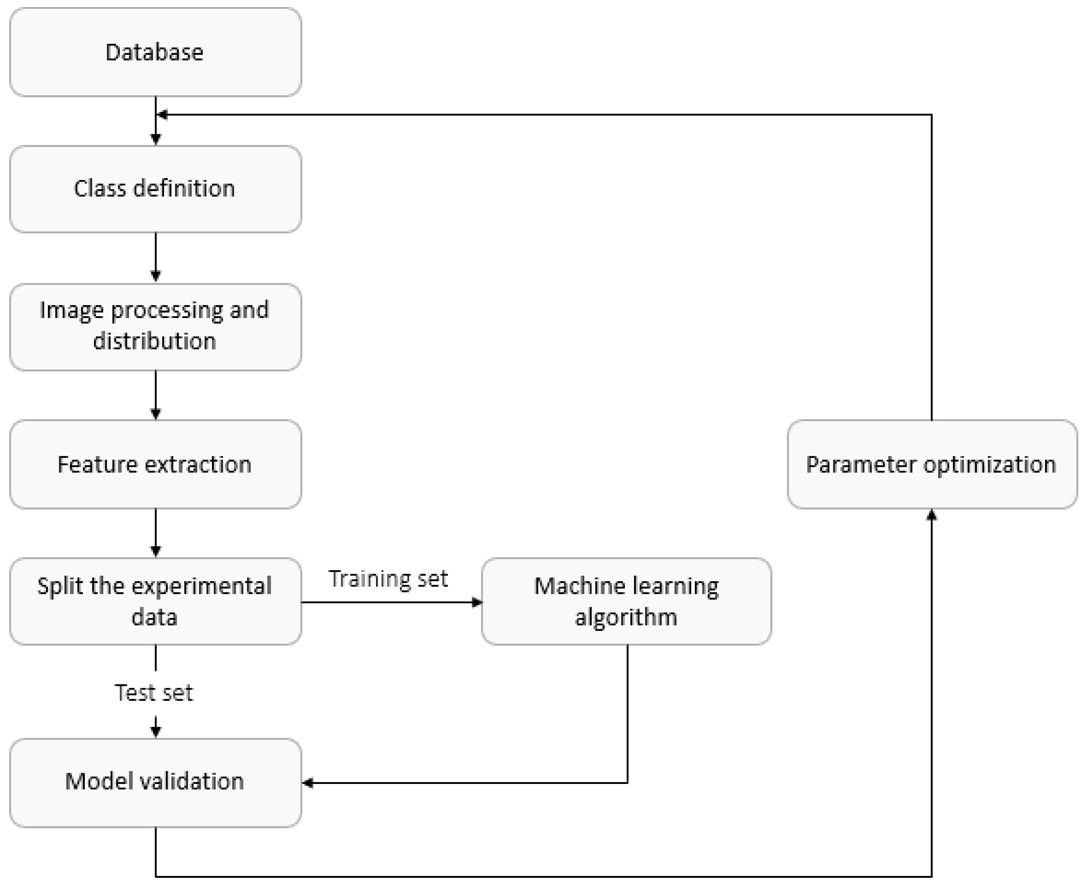
Initially, this work seeks to categorize images into several classes according to their surface roughness. Figure 3 depicts a block diagram where data processing and the training procedure are shown in detail. At this second stage, the classification learner from MATLAB software (2019b, MathWorks, Natick, MA, USA) was used.

Firstly, classes must be defined. Thus, the intervals for the arithmetic roughness, Ra, were class A [0.495, 0.799] µm, class B (0.799, 1.11] µm, and class C (1.11, 2.81] µm for three different class definitions. In this endeavor, it is necessary to collect the surface quality values from the name with which each image has been identified. In this way, it will be possible to set optimum roughness ranges to avoid imbalance in classes. As the number of groups increases, the accuracy required will be greater. Therefore, work begins on three classes. In accordance with the database used, trained models will only be able to solve classification tasks, whereas if we wanted to address regression tasks, a much larger number of images would be required.

Secondly, the photographs were processed and distributed in the specified classes. The aim of image processing is to maximize the picture features to facilitate their classification. Coloring or dimensions are some of the characteristics that were analyzed. According to the literature, machine learning algorithms based on computer vision demand a large number of samples. For this reason, the possibility of splitting images into the prediction of average values was studied in order to increase the database.

The image characteristics were then extracted by using a speeded up robust feature (SURF) detector (2019b, MathWorks, MA, USA) in order to develop a visual vocabulary. The number of attributes was modified to optimize the accuracy of the predictive model. In addition, following the supervised learning method, the name of the classes was considered as another feature.

Next, the classification learner, included in Matlab tool boxes (2019b, MathWorks, MA, USA) was invoked, a software tool capable of training supervised learning algorithms from the table of characteristics and assessing the results obtained. A portion of the feature table created for training is shown in

Table 2. Part of the feature table used by the classification learner.

Image Number	Image Features 1	Image Features 2	Image Features 3	Image Features 4	Class
1	0.0232	0.0266	0.0598	0.0730	A
2	0.0300	0.0233	0.0566	0.0933	A
3	0.0149	0.0298	0.0410	0.0298	A
4	0.0517	0.0574	0.0345	0.0345	A
5	0.0101	0.0236	0.0608	0.0642	A
6	0.0667	0.0500	0.0083	0.0917	A
7	0.0416	0.0740	0.0416	0.0694	A
8	0.0091	0.0000	0.0091	0.0000	A
9	0.0270	0.0420	0.0480	0.0960	A
10	0.0509	0.0477	0.0477	0.0668	A

, where the class column can be seen.

The support vector machine (SVM) is a supervised learning algorithm applied in countless fields to solve classification and regression problems [29]. Furthermore, following the literature [22,24,26], it has proven to be an effective technique to classify the surface roughness using higher dimensional data.

The operating principle of this classifier is based on finding an optimal hyperplane ensuring the best separation between classes, that is to say, to maximize the margin between the boundary function and the closest samples. The separation hyperplane can be defined by Equation (1), depending on its orthogonal vector w and intersection coefficient b and where x refers to the vector coordinates. Symbol T represents the transpose matrix-vector.

$$w^T\cdot x_i+b=0$$

(1)

In mathematical terms, this question becomes a quadratic programming optimization with the objective of minimizing the named margin inverse function (Equation (2)). The second term of Equation (2) represents the action of adjustment variables, ξ_i, where the C is a balancing factor.

$$\Phi \left(x\right)=\frac{1}{2}{||w||}^2+C\cdot {\sum }_{i=0}^n{\xi }_i$$

(2)

In our view, the distribution of the samples as well as the number of classes demands this issue be addressed as a higher dimensional classification with non-linear separable data. To tackle this challenge, the original area must be mapped into a higher dimensional space in order to enable developing an appropriate separation function in the new conditions. This transformation is achieved with the help of kernel functions and its effect on the problem is reflected in the SVM dual formulation (Equation (3)), where the Lagrangian is utilized to solve the quadratic programming problem and the coefficients α reference the Lagrange multipliers.

$$\Theta \left(\alpha \right)=-\frac{1}{2}\cdot {\sum }_i{\sum }_j{\alpha }_i{\alpha }_j{y}_i{y}_j\cdot {\rm K}\left(x_i{x}_j\right)-{\sum }_i{\alpha }_i$$

(3)

Kernel functions are chosen according to the nature of the problem. The suitability of different types in relation to the surface roughness prediction was discussed in the work by Abu-Mahfouz et al. [22], where a linear kernel was shown to be the most promising function. Nevertheless, all Kernel functions implemented in MATLAB^® [30] were tested in order to find that one leading the best results, i.e., the highest precision.

Finally, the validation procedure depends on the database size. In this work, two techniques were used to avoid overfitting: holdout validation and cross validation. In holdout validation, a portion of data is selected to train the predictive model, whereas the remaining samples are used as a test set. For this reason, holdout validation is suitable for large data sets. On the other hand, cross validation is characterized by the splitting of the initial samples into folds. Each block is trained with the observations not belonging to the fold and is validated with the remaining images. Test error is calculated as an average of the mistakes in each fold. Therefore, according to the number of classes and images, different validation methods were used.

4. Results and Discussion

Considering only the right answers in measuring the effectiveness of the model may lead to an erroneous perception of the machine behavior. For this reason, a confusion matrix was used to assess the performance of the supervised learning algorithms. In contrast to other metrics, a confusion matrix is capable of distinguishing between different types of errors. It is a square matrix where each row represents the actual classes, while each column refers to predicted classes. As a result, its main diagonal reflects the correct predictions, and the rest of its cells represent misclassifications.

In addition to the accuracy of the classifiers, two other measures are provided by a matrix confusion, namely precision and recall. Precision is used to obtain the percentage of correct predictions in every class, meaning the degree of reliability, while recall is used to represent the fraction of samples which were correctly recognized, that is, the model’s detection capability. Both measures were calculated using Equations (4) and (5). In these equations, TP (True Positive) refers the number of predictions where the classifier correctly predicts the positive class as positive, TN (True negative) indicates the number of predictions where the classifier correctly predicts the negative class as negative, FP (False Positive) depicts the samples incorrectly associated with a class, and FN (False Negative) represents the experiments belonging to a specific class that were wrongly labelled.

$$\mathrm{Precision}=\frac{\mathrm{TP}}{\mathrm{TP}+\mathrm{FP}}$$

(4)

$$\mathrm{Recall}=\frac{\mathrm{TP}}{\mathrm{TP}+\mathrm{FN}}$$

(5)

Combining both previous indicators, the F-score value can be obtained according to the Equation (6), which evaluates the harmonic mean of true positives and true negative cases.

$$\mathrm{F}=\frac{2\cdot \mathrm{Precision}\cdot \mathrm{Recall}}{\mathrm{Precision}+\mathrm{Recall}}$$

(6)

As discussed, the approach consisted of developing an effective model to predict the average surface roughness and to extrapolate the results to complementary variables. To this end, 153 simulations were carried out based on the procedure indicated in Figure 3. This led us to optimize the process parameters and maximize the accuracy of the predictive model. All the results are set out below, in a detailed description of the optimized model.

The model was trained with images obtained in JPG format with dimensions of 1148 × 1076 pixels, which were converted into RGB. These pictures were not split, since it has been proven that increasing the number of training images does not justify the deviation between the measured roughness and the value of the fragmented photograph. Additionally, features were extracted in each image through a SURF object recognition. At this point, the appropriate number of features was analyzed to optimize the accuracy of the model. Hence, models were trained using 2000, 1500, 1000, and 500 attributes, among other values.

In

Table 3. Comparison between the number of features extracted and the model accuracy with a medium Gaussian SVM classifier.

Model	Number of Features	Classifier	Number of Classes	Photograph Fragmentation	F-Score
91	2000	Medium Gaussian SVM	3	2 × 2	0.54
55	1500	Medium Gaussian SVM	3	2 × 2	0.57
57	1000	Medium Gaussian SVM	3	2 × 2	0.57
59	750	Medium Gaussian SVM	3	2 × 2	0.58
-	<500	Medium Gaussian SVM	3	2 × 2	>0.60

, some training tests are selected from the whole probes carried out. Particularly, those classified using Medium Gaussian SVM algorithm with three classes and using a photograph division from 1 into 4 (2 × 2) are shown. The number of features is correlated with the difficulty of classifying the photograph correctly, that is, the higher number of features, the more demanding requirements must be fulfilled. Thus, as it can be appreciated, the accuracy obtained is lower as the number of features is higher.

Finally, an initial value of 500 features was selected. In such a way, a thorough analysis could be performed to assess the impact of each characteristic on the prediction capacity, and thus counterproductive features could be removed.

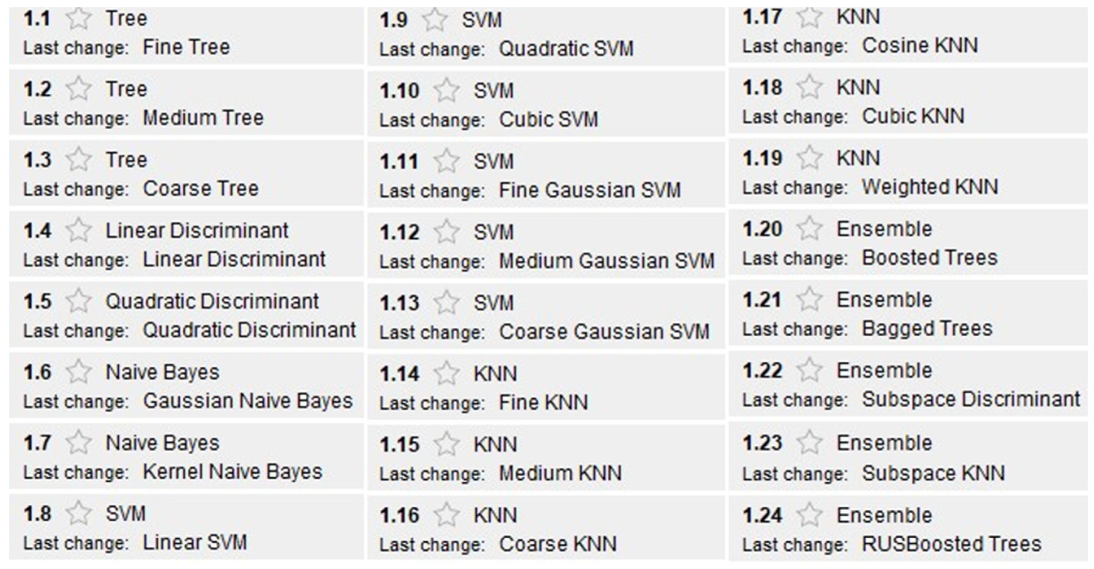
Under those conditions, all classifiers were trained. The supervised learning algorithms used to train the different models are shown in Figure 4.

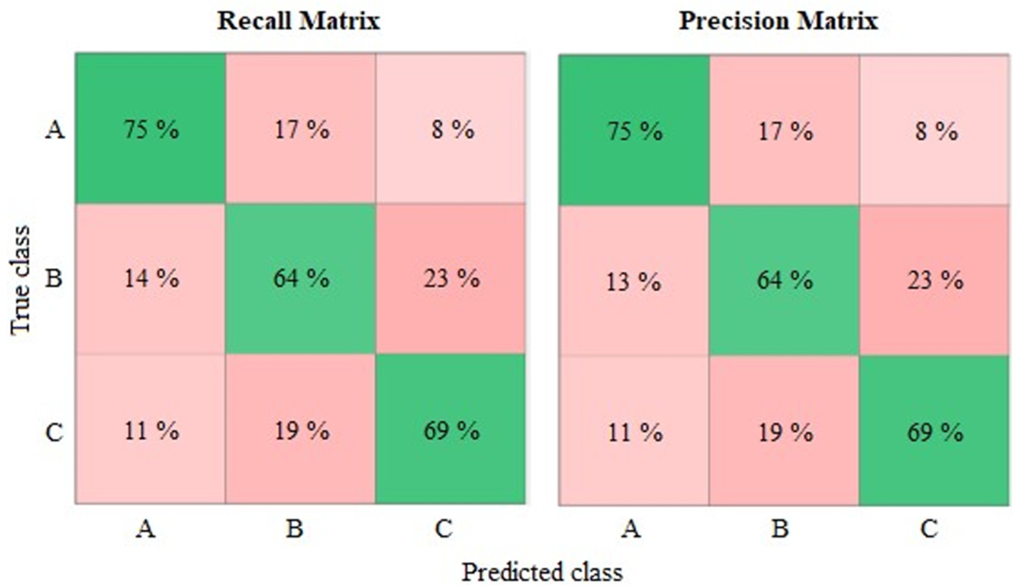
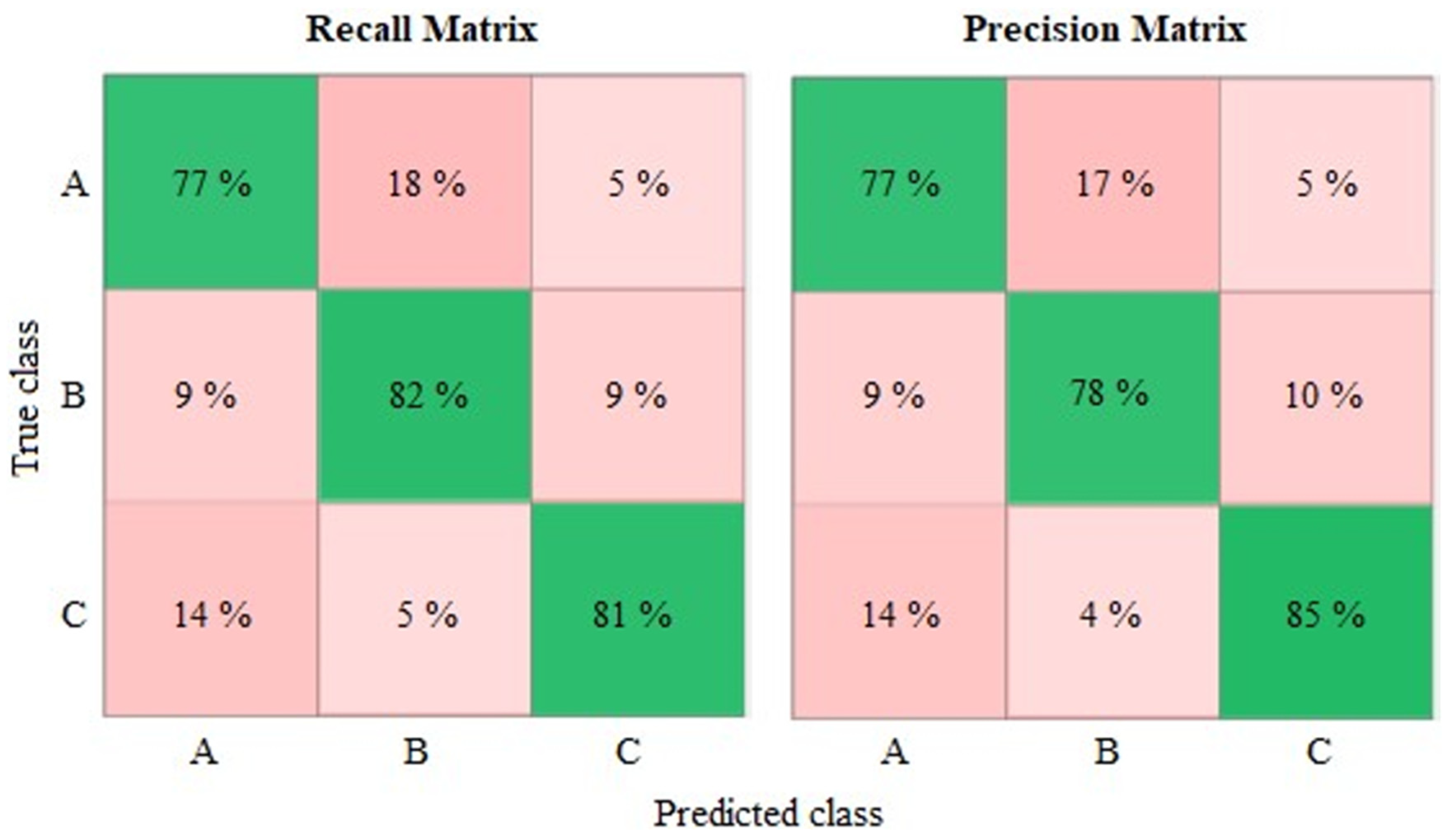
Regarding the outcome evaluation, given the limited number of training data available, a fivefold cross validation was used. Consequently, the best performance was obtained in Model 141 with a support vector machine with a quadratic kernel, the confusion matrix of which is shown in Figure 5. This model achieved an accuracy of 69.4%.

According to the recall matrix, the confusion is greater when distinguishing images belong to Classes B and C. Based on percentages, 23% of Class B images were incorrectly associated with Class C, whereas 19% of Class C samples were wrongly linked to Class B. Therefore, the predictive model displayed a better detection capability for roughness values in the first interval (Class A). Additionally, the precision matrix reflects a similar performance to that of the recall matrix, and so Class A presents the greatest reliability.

As can be seen from Figure 5, the intermediate class presented less reliability and recall with regard to the other ones, given it was more difficult to extract specific features of this class. This was a recurring issue that, among other problems, may be associated with a narrow roughness range and an insufficient database.

On the one hand, non-uniform distribution of roughness values resulted in a reduction in inequalities between categories. As a result, there are fewer specific characteristics that lead to further confusion in the classification. On the other hand, the inaccuracy of measuring instruments gains importance, since a small error, around 10 µm, might derive in an incorrect classification.

Once the average surface roughness had been studied, new predictive models were built to assess the methodology on complementary parameters, such as the maximum peak to valley height and the arithmetic mean waviness. Of these, we should highlight the following model trained to predict the average primary surface.

Model 169 was trained and validated using the same settings as the previous one. In this case, an accuracy of 80% was reached with a support vector machine with a cubic kernel. Figure 6 depicts the model confusion matrix.

As can be seen, recall and precision are approximately 80% in all classes. This improvement can be explained by the greater coherence between photographs and parameters, given that the images used represent an overlapping between roughness and waviness. In accordance with the better model performance, not only could the effectiveness of machine learning algorithms in this field be proved, but also, the application of filters on samples is considered for further work.

After running 169 simulations, changing processing parameters to build predictive models for surface quality measuring, the best results were those reported in

Table 4. Results of the models developed. Intervals for the arithmetic roughness, Ra, are: 3 classes—class A [0.495, 0.799] µm; class B (0.799, 1.11] µm; class C (1.11, 2.81] µm; 4 classes—class A [0.407, 0.7] µm; class B (0.7, 0.95] µm; class C (0.95, 1.15] µm; class D: (1.15, 2.81] µm.

Model	Variable	Classes	Classifier	Kernel	F-Score	Validation	Training Time (s)
141	Ra	3	SVM	Quadratic	0.69	Cross	1.7324
166	Ra	4	KNN	Fine	0.57	Cross	0.9927
163	Wa	3	SVM	Quadratic	0.72	Holdout	0.3857
164	Wa	4	SVM	Cubic	0.61	Holdout	1.0731
167	Rz	3	SVM	Cubic	0.56	Cross	1.6442
168	Wz	3	KNN	Cosine	0.63	Cross	0.9684
169	Pa	3	SVM	Cubic	0.80	Holdout	0.3651

.

The active participation of the support vector machine as main classifier supports the findings obtained in the literature [22,24,26]. Additionally, it is clear that this methodology is more appropriate for average parameter measuring.

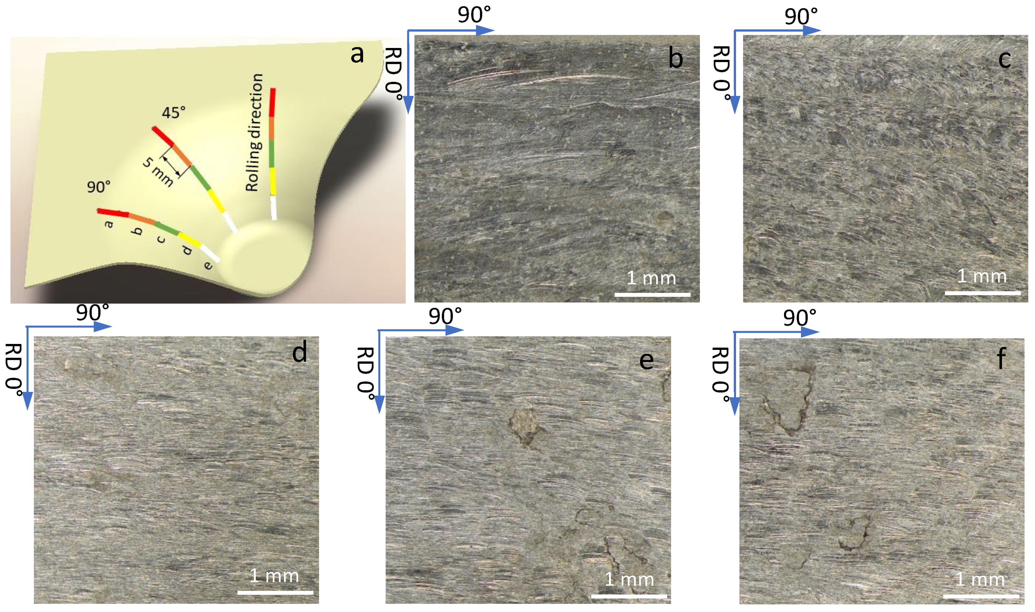
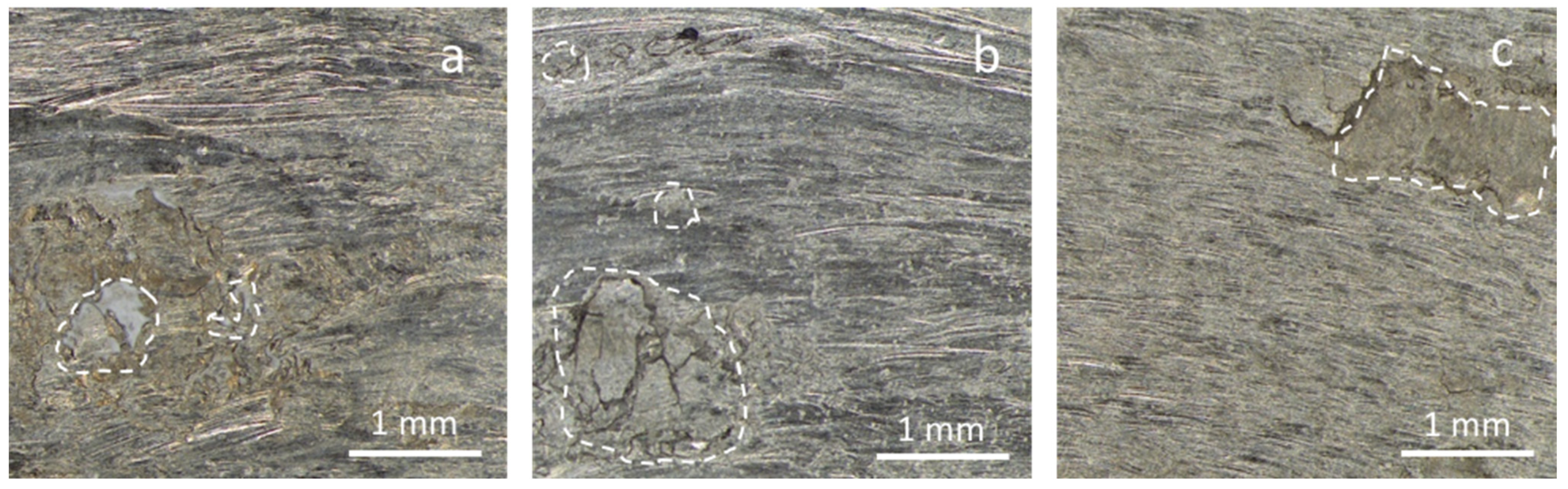
The development of this work was subject to limitations that explain the results obtained, such as the small number of training images, considering the difficulty of the feature extraction in these types of images, the narrowness of the working range and the non-uniform distribution of the roughness values. Some of these are now discussed with a view to achieving better predictive models in future works. Firstly, the working range must be taken into account. Because of the narrowness of the average surface roughness interval, specific feature extraction for each class becomes a more complex task. Moreover, a strong adhesive mechanism existed in the tribology system modelled. This involved a non-uniform surface in all the cases considered herein. Thus, the surfaces presented scattered areas with removal of material and ploughing with material accumulations, besides the typical erosive abrasive with no clear tendency across the different SPIF process conditions (Figure 7). Figure 7 depicts the surface of a part measured in a 45° direction with respect to the rolling one, in different areas. In Figure 7a, the plastic deformation caused by the overlap between passes of the tool is marked as a regular macro-ploughing effect, indicated by arrows in the image. Figure 7b shows some hints of peeling pits (some of which are marked inside circles), while in Figure 7d, some re-adhesion of previous removed material can be observed. All these phenomena contrast with an almost uniform worn surface (Figure 7c) with only a micro-ploughing phenomenon with some isolated areas of peeling pits.

Only one major adhesive mechanism was confirmed with the temperature, but its influence on the part does not always occur in the same area (Figure 7a–d). Some evidence of this can be observed in Figure 8, where the re-adhesion process is clearly noticeable in different areas of the images (marked areas). Moreover, the peeling–adhesion phenomena can dominate the topography of a study area, as can be seen in Figure 8a.

Increasing the number of observations, and thus the database size, would allow us not only to develop a margin of separation between classes, but also to define each category more accurately. While our work sets no margin, studies such as that conducted by Abu-Mahfouz et al. [22] established a distance of up to 0.18 µm between adjacent classes. As a result, classifiers based on machine vector supports using polynomial kernels achieved an 81.25% success rate.

In short, non-uniform distribution of training data demands a greater level of accuracy in both the measurement and the photography. The rigor required could be reached through the following steps:

-

Noise reduction: numerous measurements of the same area could allow more stable values to be obtained.

-

Modification of photography technique: the strategy proposed by Moreas and Bilstein [31] emphasized the relationship between the surface roughness and the peaks and valleys area. In this sense, an improvement to take into account in future work would be to use oblique illumination in an optical microscope.

Secondly, another limitation is the dataset size. The small amount of training data is a common problem in studies using machine learning algorithms. Following the literature, the number of samples required varies according to the purpose of the application. Whereas experiments using processing parameters utilize considerably fewer than a hundred observations, those using images to predict variables demand hundreds of photographs. This is evidenced by the work by Koblar et al. [23], in which 300 pictures were used to determine whether parts were suitable for commercialization in accordance with the difference between the highest peak and the lowest valley.

It is also necessary to emphasize the importance of a uniform distribution of images that allows us to use a suitable classification strategy without class imbalance. It only and exclusively depends on the manufacturing system as, in many cases, these conditions affect the surface finish of the parts in range and typology.

Finally, together with these limitations, the nature of the images must be considered. Roughness and waviness are overlapped in each photograph, so it is important to develop a filtering methodology in order to ensure that every picture faithfully represents the measured value.

5. Conclusions

In this paper, models based on machine learning were developed to predict surface quality from photographs of Ti6Al4V parts created by single point incremental forming. Training data were collected using a surface profilometer and a stereoscopic microscope, and more than one hundred and fifty simulations were run to optimize the processing parameters and to find the most suitable classifier. The main findings derived from the current work are as follows:

-

The support vector machine has proven to be a competent classifier to predict the surface finish according to the methodology used.

-

The best results are achieved using second- and third-degree polynomial kernels.

-

Working with grayscale images emphasizes the most advisable features to measure the surface roughness.

-

Dividing photographs to increase the database does not justify the deviation between images and actual values when average parameters are measured.

Overcoming the limitations of this work will provide the basis for the use of a regression model, instead of a classification one, to predict continuous values. One future direction will be to build a large and uniform database to avoid a class imbalance and to apply normalization and filtering techniques in order to obtain stable roughness values and to reduce the noise in pictures, respectively. In this way, it will be possible to build a reliable model with high detection capacity to be deployed in a productive environment.

In the future, this measuring strategy is expected to be used on real-time video transmission in a manner that enables automatic and fast selection of parts according to tolerance requirements.