Unveiling the Link between the Third Law of Comminution and the Grinding Kinetics Behaviour of Several Ores

Abstract

As a continuation of a previous research work carried out to estimate the Bond work index (w_i) by using a simulator based on the cumulative kinetic model (CKM), a deeper analysis was carried out to determine the link between the kinetic and energy parameters in the case of metalliferous and non-metallic ore samples. The results evidenced a relationship between the CKM kinetic parameter k and the grindability index gbp; and also with the w_i, obtained following the standard procedure. An excellent correlation was obtained in both cases, posing the definition of alternative work index estimation tests with the advantages of more straightforward and quicker laboratory procedures.

1. Introduction

The importance of work index determinations in mineral ores comminution operations is without any doubt. The methodology proposed by F.C. Bond [1] is widely used in grinding equipment design and calculations. The crucial point is that it was developed on an enormous data quantity, both at laboratory and industrial scales, yielding sound and reliable results. This fact provided Bond’s methodologies with great prestige from its inception and, despite many attempts to develop a technique to replace it over time, it established itself as an essential tool for design and sizing the reduction stages of hundreds of metallurgical plants around the world.

However, the Bond proposal has some shortcomings, pointed out by Gutierrez and Sepulveda [2], Aksani and Sömmez [3] and Menendez Aguado et al. [4], which are summarized below:

• Availability of the standard mill
• Availability of a minimum sample of 10 kg
• Excessive duration of the procedure (in case of some ores)
• Lack of detailed procedure definition (there is no ASTM or ISO specific standard)

These shortcomings have fostered the proposal of alternative grindability characterization procedures. Thus, Lvov and Chitalov [3] performed an in-depth review of several alternative methodologies. Recently, Josefin and Doll [4] proposed an alternative methodology to obtain w_i at a different closure size (P₁₀₀) than the one tested, and Nikolić and Trumić [5] proposed an alternative procedure when the feed top size (F₁₀₀) is much lower than 3.35 mm, the top size referenced in the Bond standard methodology (BSM). Moreover, estimating the work index variability from the variability of the geomechanical parameters is the central idea of several alternative procedures, as recently proposed by Park and Kim [6]; this mine-to-mill approach needs further development, but opens a promising way related to mine digitalization strategies for process optimization. Currently, new tools are being developed to estimate w_i, some of which stand out for the reuse of equipment applying modern technologies, simplifying methodologies or applying mathematical models, as it is the case of the following authors:

• Aksani et al. [7] proposed a methodology to obtain the work index by simulation using the CKM and showed results for six different ores, reporting deviations less than 4%.
• Menéndez Aguado et al. [8] showed an alternative methodology based on a non-standard mill, reporting a mean square error of less than 3%.
• Ahmadi et al. [9] presented a methodology with an industrial-scale validation; deviations reported in this case were less than 7%.
• Mwanga et al. [10,11] developed an alternative small sample methodology (300 g) with a geometallurgical approach, reporting mean square error less than 5%.
• Heiskari et al. [12] also presented an alternative methodology using a small sample quantity in a Mergan mill, as an evolution of the former proposal of Niiti [13]. The deviation values reported in this case were less than 4%.

Moreover, Ciribeni et al. [14] proposed a simplified technique to determine the CKM kinetic grinding parameters in order to simulate the Bond test and to validate it by contrasting the results of Au and Ag metalliferous ore samples from various deposits in the Argentine Patagonia. At present, the application of mathematical models to simulate grinding has proven to be a helpful tool for determining the work index, not only in the abovementioned case of Aksani et al. [7], but also in previous work from Lewis et al. [15] and more recently Silva et al. [16]. However, only some authors present alternatives that solve the difficulties of Bond’s procedure. This method allows testing with a small sample, especially when looking to obtain the work rate of drill core samples, limiting the sample size to less than a pair of kilograms. This is usually the case of practical geometallurgy, which provides data for the economic and technical evaluation of mineral exploitation and the metallurgical plant, and seeks to predict the mineral behaviour in the metallurgical processes.

The simulator developed by Ciribeni et al. [14] allowed the estimation w_i from the CKM kinetic parameters with a good approximation. Deniz [17] studied the relationship among the Bond standard test parameters and the kinetic parameters following the well-known Austin methodology [18], suggesting several relationships between the grindability index gbp and the set of kinetic data. However, this work was carried out only on one ore, and the practical advantage of this solution is not convenient, given that the determination of Austin parameters can involve even more laboratory work than in the test defined by the BSM in the case of ball mills. Moreover, several papers have been published studying the deviations from the linear kinetic approach [19,20]. However, the CKM procedure provides a quick parameter determination.

Hence, the objective of this research was to study the relationship between the CKM kinetic parameters and the Bond ball mill standard test parameters (gbp, w_i) to propose alternative methodologies of work index estimation with practical advantages. The main hypothesis is that, as suggested by Deniz [17], there can be found a relationship between the CKM kinetic parameter k and the power consumption parameters in the BSM, such as gbp and w_i.

2. Materials and Methods

2.1. The Cumulative Kinetic Model

The cumulative kinetic model is the simple solution defined by Laplante [21], for the equation proposed by Loveday [22] as a first-order kinetic equation. The particle breakage rate in a given size interval is proportional to the mass present in this interval. The kinetic parameter k is defined by the disappearance rate of oversize particles for a given size class (for both batch or continuous grinding—assuming a plug flow regime in the latter one) and can be described with the CKM model as expressed in Equation (1).

$$W_{\left(x,t\right)}=W_{\left(x,0\right)}\exp \left(-k·t\right)$$

(1)

wherein:

• W(x,t) = cumulative percentage of oversize of size class x at time t.
• W(x,0) = cumulative percentage of oversize of size class x in the fresh feed.
• k = breakage rate constant (min⁻¹)
• t = time, (min)

The equation that describes the relationship between the breakage rate and the particle size is shown in Equation (2):

$$k=C·x^n$$

(2)

wherein C and n are constants, dependent on the characteristics of the ore and the mill, as described by Ersayin et al. [23]. C and n can be determined experimentally and once known the feed particle size distribution (PSD) the product PSD can be calculated by means of Equation (3).

$$W_{\left(x,t\right)}=W_{\left(x,0\right)}\left(\exp \left(-C·x^n·t\right)\right)$$

(3)

2.2. Kinetic Parameters Determination

Kinetic parameter k is determined with a small sample in a laboratory mill, as described in [14]. In this case, the standard mill designed by Bond is used to avoid introducing this uncertainty factor when simulating the Bond standard test.

With the same amount of feed from the Bond test (700 cm³), successive grinding runs are carried out at pre-established time intervals. Once finished each run, a representative sample of the mineral load is taken, and the product PSD is obtained; the sample is returned to the mill, recomposing the load and allowing the performance of the subsequent grinding run.

To simplify this test, the simplified methodology (SIM) presented in [14] proved that a single grinding run could be made to determine the kinetic parameter k, saving time and avoiding excessive manipulation of the sample. The k value is determined for different monosizes, making the linear regression of the cumulative retained for the final milling time, using Equation (4):

$$\mathrm{Ln}\left(W_{\left(x,t\right)}\right)-\mathrm{Ln}\left(W_{\left(x,0\right)}\right)=kt$$

(4)

2.3. Experimental Procedure

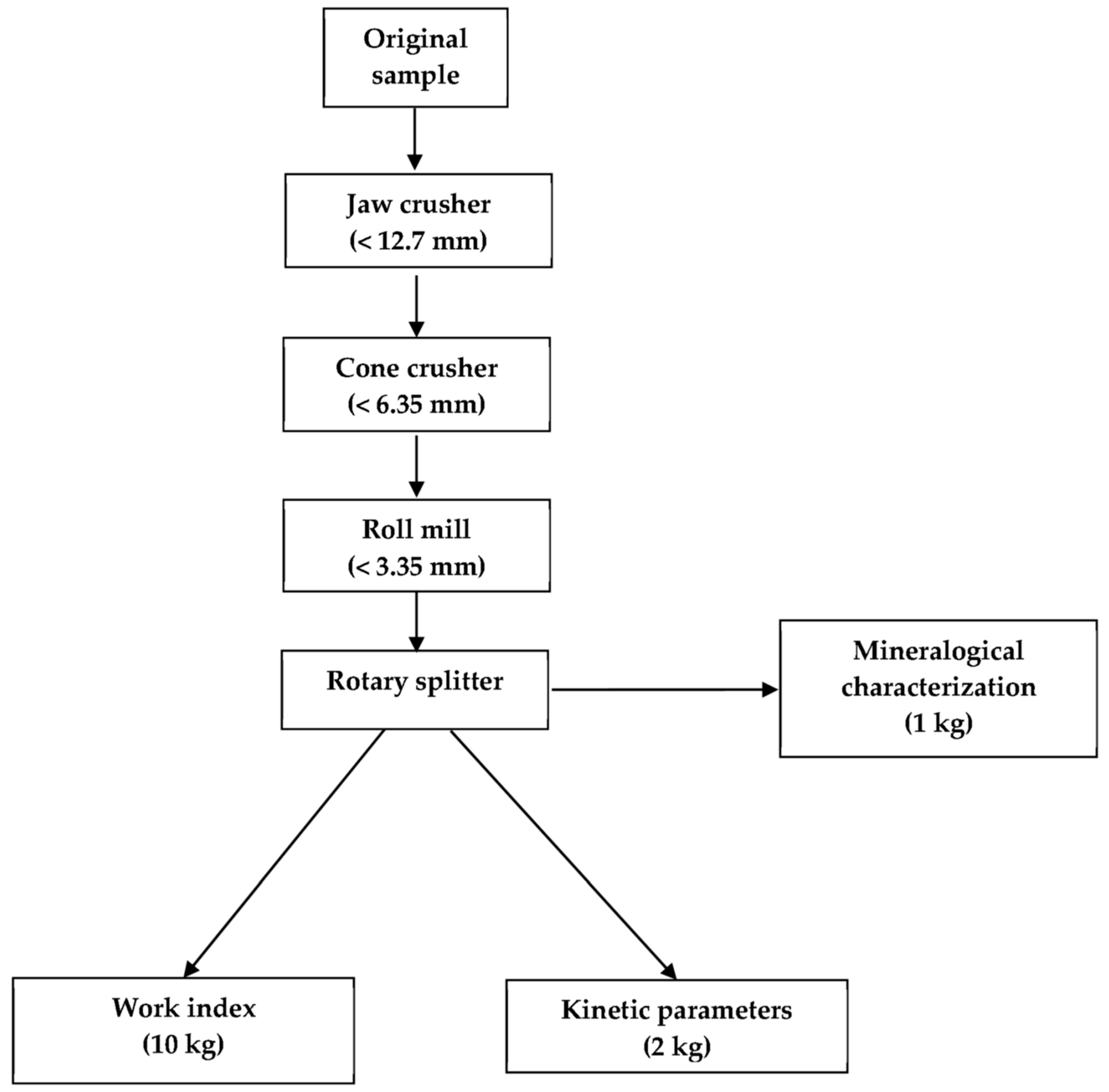
2.3.1. Sample Preparation

For this work, samples from three metalliferous ores from Argentine Patagonia were selected and prepared according to the conventional preparation scheme used to prepare the feed in a Bond’s ball mill standard test (Figure 1). In each case, the sample amount prepared was enough to carry out the SIM tests to obtain the kinetic parameters k [14] and also to obtain the BSM work index [1], which will be used for validation purposes.

PSD were obtained in a Ro-Tap sieve with sieves 203 mm in diameter (ASTM certified). Sampling was carried out in a Sieving Riffler Quantachrome eight sector rotary sampler.

2.3.2. Sample Characterization

To perform this study, data from Ciribeni et al. [14] were used. However, some additional ores were considered in this research and are included below.

The new samples came from metalliferous deposits (Au, Ag) from the metallogenetic province “Macizo del Deseado” (Argentine Patagonia):

• Low sulphidation (LS) ore: several samples were taken from this ore, which comes from a low sulphidation hydrothermal deposit, formed mainly by veins of silica in the form of quartz, chalcedony and opal; native gold is present, and silver can be found in a wide range of minerals (electrum, sulfosalts, cassiterite, galena, pyrite and chalcopyrite, among other minerals).
• High sulphidation (HS) ore: comes from deposits of the epithermal type of medium sulphidation, which is made up of quartz, carbonates and to a lesser extent Au, and Ag sulphides and sulphosalts, in addition to Pb, Cu and Zn.

2.3.3. Determination of Kinetic Parameters and Work Index

The kinetic parameter k was determined following the SIM methodology [14]. It is carried out in a Bond standard ball mill, with sample feed 700 cm³ (prepared according to the procedure presented in Figure 1). After PSD feed determination, a sole 5 min grinding run is performed, and the product PSD is obtained. This grinding time value was selected considering that grinding runs in the Bond standard test do not usually exceed 350 revolutions (5 min, at 70 rpm). For each size interval, k is calculated (Equation (4)). Using Equation (2) for that set of k and x values, C and n for each ore are calculated, and an estimation of work index by CKM simulation, w_i,s, is performed [14].

The Bond work index (w_i) was determined following BSM, the standard methodology developed by F. C. Bond [1]. The ball mill work index laboratory test is conducted by grinding an ore sample prepared to 100% passing 3.36 mm to product size in the range of 45–150 µm, thus determining the ball mill w_i. Several sources of variability, mainly due to a lack of procedure definition were identified by García et al. [24]. With the aim of reducing that variability, a detailed description of the test can be found in the proposal of the Global Mining Guidelines Group [25].

3. Results and Discussion

3.1. Work Index Calculation and Estimation

Table 1. Comparison between w_i and w_i,s for different metalliferous ores.

Sample	P100	wi [kWh/t]	wi,s [kWh/t]	Difference [%]
LS-CMLM1	74	26.59	27.63	−3.91
LS-CMVM1	74	25.17	24.56	2.42
HS-CCTUM1	149	13.82	12.96	6.22

shows the actual BSM w_i values obtained versus the work index estimation by CKM simulation (w_i,s). LS-CMLM1 and LS-CMVM1 samples were tested at a reference size P₁₀₀ = 74 µm; estimated values by simulation differ less than 4%. Meanwhile, HS-CCTUM1 sample was tested at P₁₀₀ = 149 µm, and the estimation difference with the actual w_i value was rounded by 6%.

Results of w_i and w_i,s calculations in the considered samples from previous research [9] complete the subsequent

Table 2. Grindability and kinetic parameters obtained experimentally.

Sample	P100 [µm]	F80 [µm]	P80 [µm]	wi [kWh/t]	gbp [g/rev]	k (@ P100)
LS-CMLM1	74	1938	54	26.59	0.8038	0.03667
LS-CMVM1	74	2053	53	25.17	0.6907	0.03656
HS-CCTUM1	149	2469	96	13.82	1.3427	0.12543
LS-CNM1	149	2508	113	21.17	1.0176	0.06539
HS-CVM1	149	2284	115	16.31	1.4784	0.09132
LS-CVM2	149	2432	116	17.57	1.2500	0.08693
LS-CVM3	149	2333	114	19.08	1.1180	0.08143
Quartz	149	2572	117	15.27	1.5773	0.10141
Quartz	105	2552	83	19.89	1.1048	0.06492
Feldspar	149	1841	115	13.65	1.9112	0.13860
Feldspar	105	1676	81	16.16	1.3567	0.09183
Limestone	149	2407	108	10.88	2.2533	0.15128
Calcite	149	2497	112	6.93	3.9221	0.25711
Cryst. limestone	149	2062	112	8.46	3.3308	0.20919
Cryst. limestone	105	1926	79	10.91	2.2591	0.14956

and

Table 3. Comparison w_i versus w_i,e1.

Sample	P100 [µm]	wi [kWh/t]	gbp [g/rev]	wi,e1 [kWh/t]	gbpe [g/rev]	Difference [%]
LS-CMLM1	74	26.59	0.8038	24.84	0.5869	6.59
LS-CMVM1	74	25.17	0.6907	24.48	0.5852	2.73
HS-CCTUM1	149	13.82	1.3427	11.23	1.8863	18.73
LS-CNM1	149	21.17	1.0176	20.77	1.0073	1.88
HS-CVM1	149	16.31	1.4784	16.37	1.3869	−0.39
LS-CVM2	149	17.57	1.2500	16.97	1.3226	3.44
LS-CVM3	149	19.08	1.1180	17.77	1.2422	6.88
Quartz	149	15.27	1.5773	15.09	1.5211	1.15
Quartz	105	19.89	1.1048	18.65	1.0003	6.24
Feldspar	149	13.65	1.9112	12.15	2.0790	11.00
Feldspar	105	16.16	1.3567	14.74	1.3944	8.78
Limestone	149	10.88	2.2533	10.44	2.2647	4.00
Calcite	149	6.93	3.9221	6.94	3.8140	−0.10
Cryst. limestone	149	8.46	3.3308	8.42	3.1125	0.45
Cryst. limestone	105	10.91	2.2591	9.66	2.2395	11.48

.

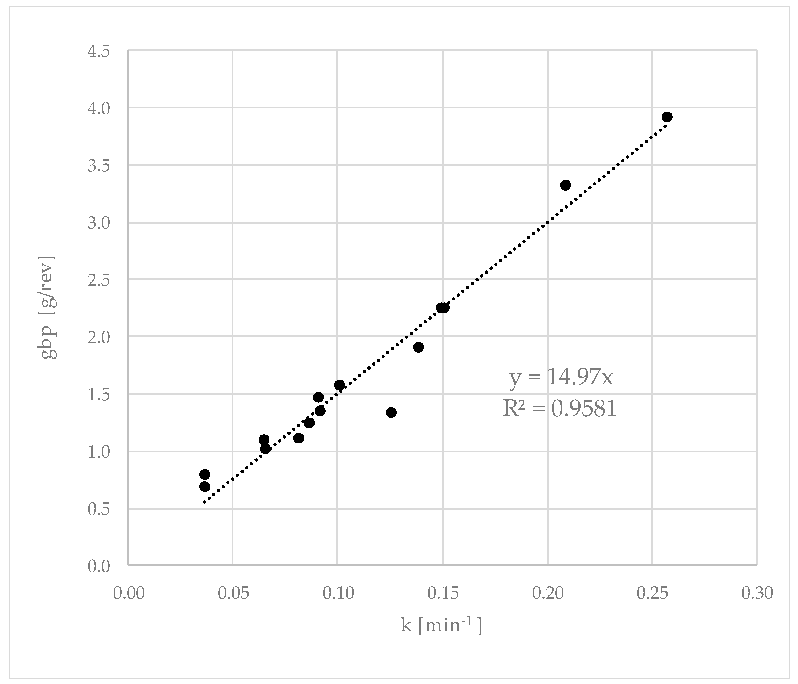
3.2. Relationships between Grindability and Kinetic Constant k

Table 2 summarises the work indices determined by BSM and estimated by CKM with kinetic indices k determined by the SIM procedure. The considered metalliferous ore samples came from the current research tests and the former research ones. Some non-metallic minerals from the former research are also included. All data are used to unveil the links between BSM parameters and those obtained by grinding kinetics (SIM).

After plotting gbp (determined with the standard procedure) versus the kinetic parameter k (calculated by the SIM methodology), as is shown in Figure 2, a linear estimation can be obtained (Equation (5)) with a correlation coefficient of 95.8%.

$$gbp=14.97·k$$

(5)

According to the BSM procedure, w_i can be calculated for each P₁₀₀ once gbp, F₈₀ and P₈₀ are known. A new work index estimation, w_i,e1, can be suggested considering the gbp estimated value (gbp_e) in Equation (5), and F₈₀ and P₈₀ estimated by the SIM procedure, in each case. Table 3 shows the results obtained from this new estimation proposal, wherein work index differences are in general less than 10% for each ore. However, there are three values above 10% and one reaching 18%.

Figure 3 depicts the relationship of w_i versus w_i,e1; a linear correlation (Equation (6)) can be plotted, with a correlation coefficient of 98.22%.

$$w_i=0.962·w_{i,e1}-0.28$$

(6)

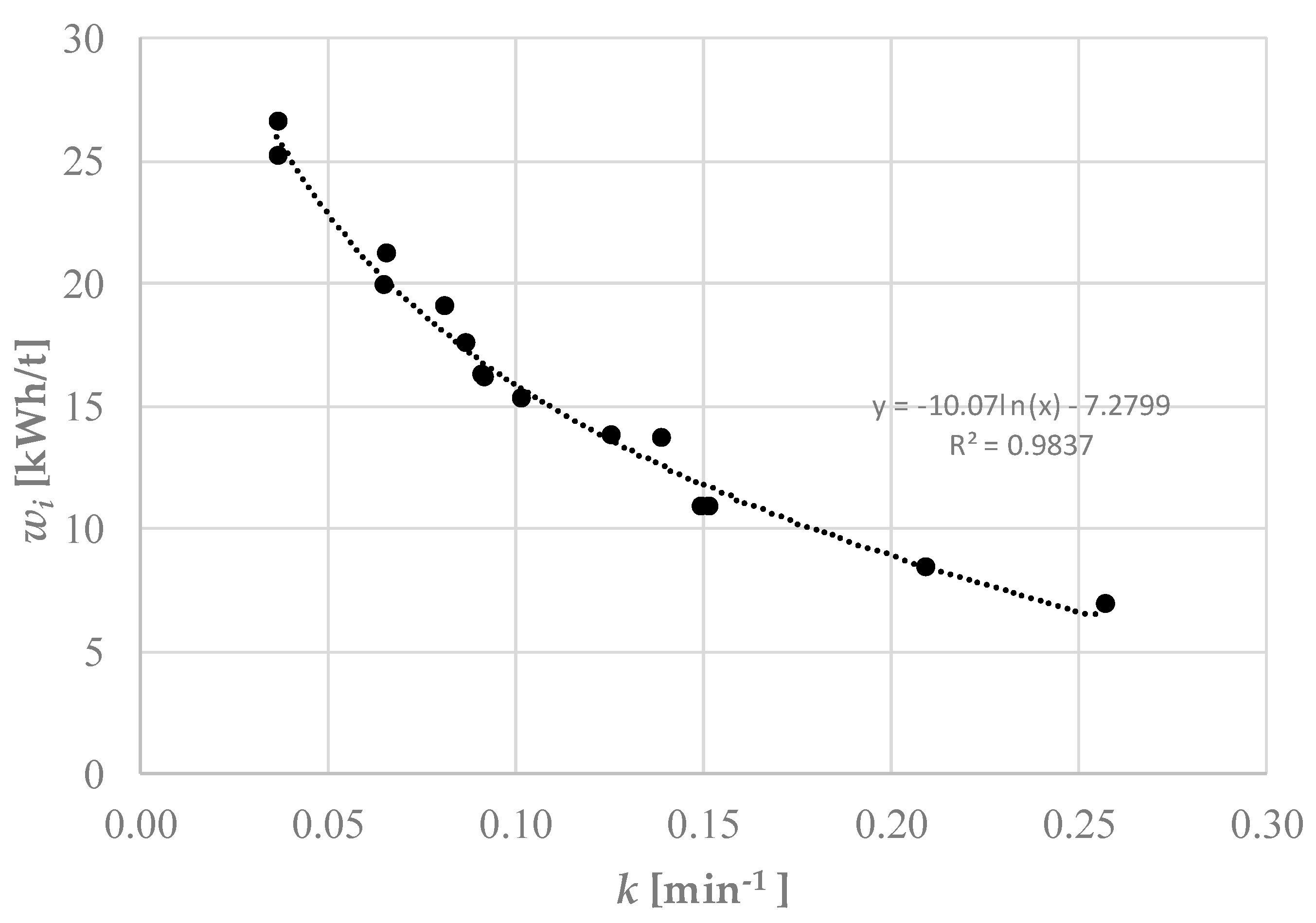
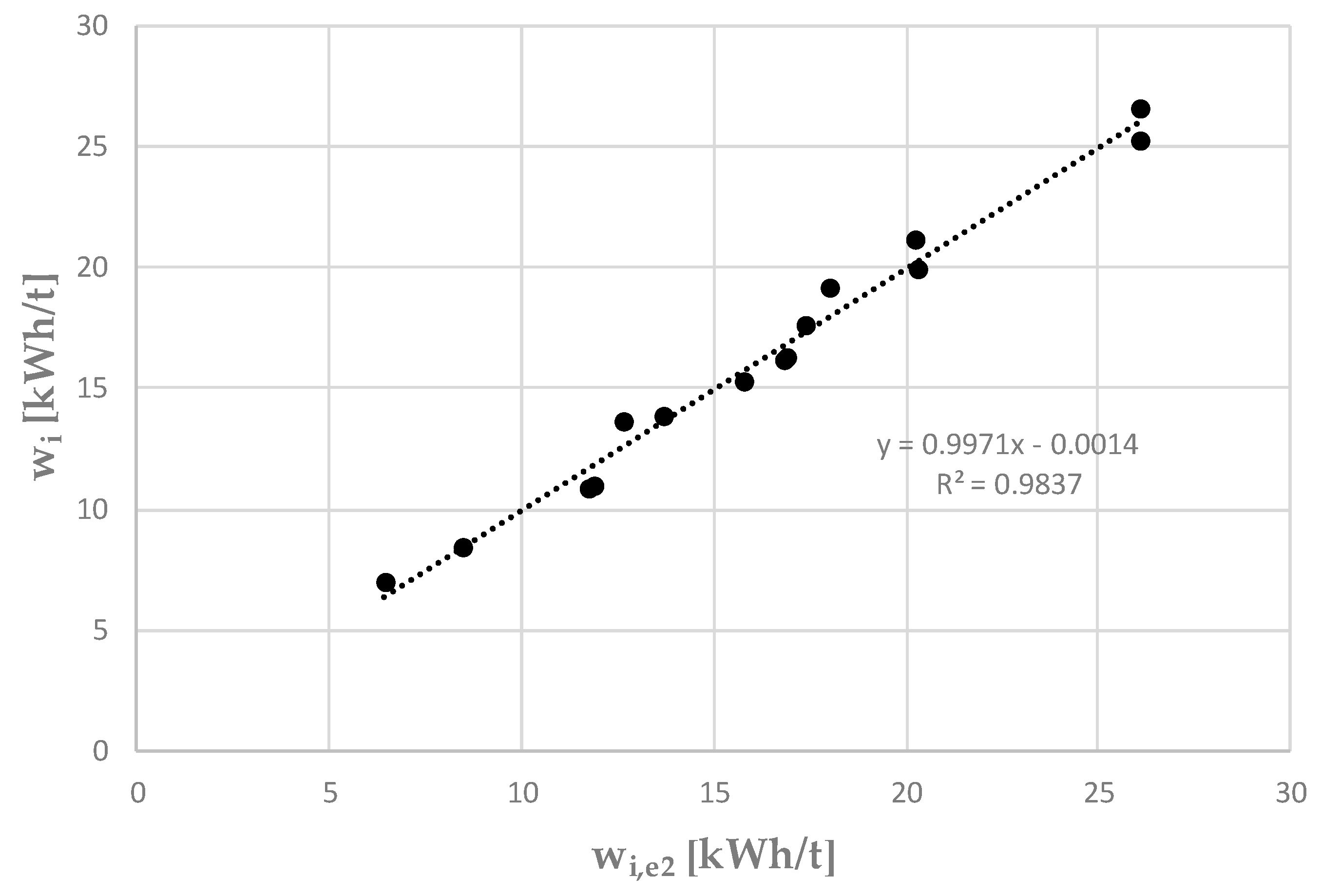
3.3. Linking the Work Index w_i and the Kinetic Constant k

As a consequence of the relationships evidenced in Equations (5) and (6), it can be inferred that there should be a correlation between the Bond work index and the kinetic constant k at each monosize. Figure 4 depicts this relationship between w_i and k from the actual data gathered in Table 2, wherein a logarithmic correlation (Equation (7)) poses a correlation coefficient of 98.37%.

$$w_i=-10.07·\ln \left(k\right)-7.28$$

(7)

Table 4. Comparison between w_i and work index estimation using Equation (7), w_i,e2.

Sample	P100 [µm]	wi [kWh/t]	k [@P100]	wi,e2 [kWh/t]	Difference [%]
LS-CMLM1	74	26.59	0.03667	26.09	1.89
LS-CMVM1	74	25.17	0.03656	26.12	−3.77
HS-CCTUM1	149	13.82	0.12543	13.67	1.10
LS-CNM1	149	21.17	0.06539	20.25	4.36
HS-CVM1	149	16.31	0.09132	16.87	−3.45
LS-CVM2	149	17.57	0.08693	17.37	1.13
LS-CVM3	149	19.08	0.08143	18.03	5.50
Quartz	149	15.27	0.10141	15.81	−3.57
Quartz	105	19.89	0.06492	20.32	−2.16
Feldspar	149	13.65	0.13860	12.66	7.26
Feldspar	105	16.16	0.09183	16.82	−4.06
Limestone	149	10.88	0.15128	11.78	−8.23
Calcite	149	6.93	0.25711	6.42	7.38
Cryst. limestone	149	8.46	0.20919	8.50	−0.49
Cryst. limestone	105	10.91	0.14956	11.89	−8.99

shows a comparison of actual work index values versus work index estimation using Equation (7); in all cases, differences are lower than 9%.

In Figure 5, the estimated work index using Equation (7) w_i,e2 is plotted versus w_i, revealing the unexpected linear correlation shown in Equation (8), with a correlation coefficient of 98.37%

$$w_i=0.997·w_{i,e2}-0.001$$

(8)

3.4. Discussion

Table 1 presented the work index estimation by CKM simulation (w_i,s) versus the actual w_i values, in the case of three different samples. Results show deviations less than 6%. This procedure saves laboratory time (8 to 2 h, approximately) and reduces sample needs from 10 kg to less than 1.5 kg.

Intending to get a more significant reduction, the research work focused on searching for a correlation between the k kinetic parameter, determined by the SIM methodology developed by Ciribeni et al. [10], and the grindability index, gbp. As can be observed in Figure 2, a good linear correlation (Equation (5)) was obtained, opening the possibility of estimating gbp from the k value (which can be obtained in the laboratory more easily and quickly) and thus providing a new proposal of work index estimation, w_i,e1.

In Table 3, the comparison between w_i (Bond work index value obtained following the BSM) and w_i,e1 showed differences, in general, lower than 9%, being in some cases greater than 10%, even reaching 18% in one specific case. This fact can raise the consideration that this methodology is a bit erratic.

On the other hand, the study of the relationship between w_i and k presents an adjustment to a logarithmic function with a correlation coefficient higher than 98%, which is more than acceptable considering that this result was obtained adjusting data of fifteen actual w_i determinations on different ores and with different P₁₀₀. The estimation of w_i using Equation (7) posed differences lower than 9% in all cases and for all reference sizes. Moreover, in Table 4, it is observed that in the case of metalliferous ores, differences are below 5.50%, with higher variability in the case of non-metalliferous ones. Amadi and Shahsavari [9] reported deviations lower than 7%, and Aksani and Sönmez reported values lower than 4%, using in both cases the CKM simulation-based methodology, that is, in the same order of magnitude.

According to results depicted in Figure 5, where the linear fitting (Equation (8)) casts a correlation coefficient higher than 98% with a slope very close to one and an almost zero intercept, it seems feasible and accurate enough to perform the work index estimation at a given P₁₀₀, just by knowing the kinetic parameter k obtained at P₁₀₀ and by using Equation (7).

The combination of the SIM methodology [14] with the correlation of k and w_i provides a quick solution, with a minimum sample amount needed, in order to estimate the work index. An additional advantage is the reduction of procedures involving sample manipulation and quartering at the lab, which are usual sources of experimental error.

4. Conclusions

From the results obtained in this research, the following conclusions can be highlighted:

• Once the CKM kinetic parameter k for the given reference sieve P₁₀₀ was known, it was possible to estimate the BSM ball mill work index at that reference size, with differences lower than 9% with the Bond standard methodology.
• It was found that a linear fit yielded a correlation coefficient higher than 96% between gbp and the kinetic parameter k (Equation (5)). The line has slope fifteen and zero intercept. However, estimating w_i by determining gbp with Equation (5) and calculating w_i with the Bond equation gives some erratic values.
• With fifteen different ore samples and for three different P₁₀₀, a logarithmic correlation w_i versus k was obtained (Equation (7)) with a correlation coefficient higher than 98%. It can be suggested that the logarithmic function in Equation (7) could be a valuable tool as a quick alternative to Bond’s standard test in the day-by-day grindability control.
• The comparison between w_i and w_i,e2 (Equation (8)) shows a linear fit whose slope is unity and the ordinate to the origin is negligible, with a correlation coefficient higher than 98%.
• The use of k versus w_i correlation provides a quick solution, with a minimum sample amount need, in order to estimate the work index.

References

1. Bond, F.C. Crushing and grinding calculations. Part I. Br. Chem. Eng. 1961, 6, 378–385. [Google Scholar]
2. Gutiérrez, L.; Sepúlveda, J. Dimensionamiento y Optimización de Plantas Concentradoras, Mediante Técnicas de Modelación Matemática; CIMM: Santiago, Chile, 1986. [Google Scholar]
3. Valerevich Lvov, V.; Sergeevich Chitalov, L. Comparison of the Different Ways of the Ball Bond Work Index Determining. Int. J. Mech. Eng. Technol. 2019, 10, 1180–1194. Available online: https://ssrn.com/abstract=3452642 (accessed on 2 July 2021).
4. Nikolić, V.; Trumić, M. A new approach to the calculation of Bond work index for finer samples. Miner. Eng. 2021, 165, 106858. [Google Scholar] [CrossRef]
5. Josefin, Y.; Doll, A.G. Correction of Bond Ball Mill Work Index Test for Closing Mesh Sizes. Procemin-Geomet 2018. In Proceedings of the 14th International Mineral Processing Conference & 5th International Seminar on Geometallurgy, Santiago, Chile, 28–30 November 2018; pp. 1–12. [Google Scholar]
6. Park, J.; Kim, K. Use of drilling performance to improve rock-breakage efficiencies: A part of mine-to-mill optimization studies in a hard-rock mine. Int. J. Min. Sci. Technol. 2020, 30, 179–188. [Google Scholar] [CrossRef]
7. Aksani, B.; Sönmez, B. Simulation of Bond grindability test by using cumulative based kinetic model. Miner. Eng. 2000, 13, 673–677. [Google Scholar] [CrossRef]
8. Menéndez-Aguado, J.M.; Dzioba, B.R.; Coello-Velazquez, A.L. Determination of work index in a common laboratory mill. Miner. Metall. Process. 2005, 22, 173–176. [Google Scholar] [CrossRef]
9. Ahmadi, R.; Shahsavari, S. Procedure for determination of ball Bond work index in the commercial operations. Miner. Eng. 2009, 22, 104–106. [Google Scholar] [CrossRef]
10. Mwanga, A.; Rosenkranz, J.; Lamberg, P. Testing of ore comminution behavior in the geometallurgical context: A review. Minerals 2015, 5, 276–297. [Google Scholar] [CrossRef] [Green Version]
11. Mwanga, A.; Rosenkranz, J.; Lamberg, P. Development and experimental validation of the Geometallugical Comminution test (GCT). Miner. Eng. 2017, 108, 109–114. [Google Scholar] [CrossRef]
12. Heiskari, H.; Kurki, P.; Luukkanen, S.; Gonzalez, M.; Lehto, H.; Liipo, J. Evelopment of a comminution test method for small ore samples. Miner. Eng. 2019, 130, 5–11. [Google Scholar] [CrossRef]
13. Niitti, T. Rapid evaluation of grindability by a simple batch test. In Proceedings of the International Mineral Processing Congress Proceedings, Prague, Czech Republic, 1–6 June 1970; pp. 41–46. [Google Scholar]
14. Ciribeni, V.; Bertero, R.; Tello, A.; Puertas, M.; Avellá, E.; Paez, M.; Menéndez Aguado, J.M. Application of the Cumulative Kinetic Model in the Comminution of Critical Metal Ores. Metals 2020, 10, 925. [Google Scholar] [CrossRef]
15. Lewis, K.A.; Pearl, M.; Tucker, P. Computer Simulation of the Bond Grindability Test. Miner. Eng. 1990, 3, 199–206. [Google Scholar] [CrossRef]
16. Silva, M.; Casali, A. Modelling SAG Milling Power and Specific Energy Consumption Including the Feed Percentage of Intermediate Size Particles. Miner. Eng. 2015, 70, 156–161. [Google Scholar] [CrossRef]
17. Deniz, V. Relationships Between Bond’s Grindability (Gbg) and Breakage Parameters of Grinding Kinetic on Limestone. Powder Technol. 2004, 139, 208–213. [Google Scholar] [CrossRef]
18. Austin, L.G.; Klimpel, R.R.; Luckie, P.T. Process Engineering of Size Reduction: Ball Milling; SME-AIME: New York, NY, USA, 1984. [Google Scholar]
19. Bilgili, E.; Scarlett, B. Population balance modeling of nonlinear effects in milling processes. Powder Technol. 2005, 153, 59–71. [Google Scholar] [CrossRef]
20. Petrakis, E.; Komnitsas, K. Development of a Non-linear Framework for the Prediction of the Particle Size Distribution of the Grinding Products. Min. Metall. Explor. 2021, 38, 1253–1266. [Google Scholar]
21. Laplante, A.R.; Finch, J.A.; del Villar, R. Simplification of Grinding Equation for Plant Simulation. Trans. Inst. Min. Metall. (Sect. C) 1987, 96, C108–C112. [Google Scholar]
22. Loveday, B.K. An analysis of comminution kinetics in terms of size distribution parameters. J. S. Afr. Inst. Min. Metall. 1967, 68, 111–131. [Google Scholar]
23. Ersayin, S.; Sönmez, B.; Ergün, L.; Aksani, B.; Erkal, F. Simulation of the Grinding Circuit at Gümüsköy Silver Plant, Turkey. Trans. Inst. Min. Metall. (Sect. C) 1993, 102, C32–C38. [Google Scholar]
24. García, G.G.; Oliva, J.; Guasch, E.; Anticoi, H.; Coello-Velázquez, A.L.; Menéndez-Aguado, J.M. Variability Study of Bond Work Index and Grindability Index on Various Critical Metal Ores. Metals 2021, 11, 970. [Google Scholar] [CrossRef]
25. GMG—Global Mining Guidelines Group. Determining the Bond Efficiency of Industrial Grinding Circuits. 2016. Available online: https://gmggroup.org/wp-content/uploads/2016/02/Guidelines_Bond-Efficiency-REV-2018.pdf (accessed on 1 July 2021).
Figure 1. Samples preparation flowsheet.
Metals 11 01079 g001
Figure 2. Plot gbp (BSM) versus k (SIM).
Metals 11 01079 g002
Figure 3. Linear correlation between wi and wi,e1.
Metals 11 01079 g003
Figure 4. Logarithmic correlation wi versus k.
Metals 11 01079 g004
Figure 5. Linear correlation wi versus wi,e2.
Metals 11 01079 g005