Metallurgical Modelling of Ti-6Al-4V for Welding Applications

Abstract

Manufacturing processes such as welding subject the α/β titanium alloy Ti-6Al-4V to a wide range of temperatures and temperature rates, generating microstructure variations in the phases and in the precipitate dimensions. In this study, the metallurgical and numerical modelling of Ti-6Al-4V when subjected to a high energy density welding process was affected by a series of analytical equations coded in Sysweld commercial specialist FE welding software. Numerical predictions were compared with experimental results from laser welding tests on plates with different thicknesses, initial microstructural morphologies, and operating conditions. The evolution of the microstructure was described by using a diffusion-based approach when the material was operating in the α + β field, whilst empirical equations were used for temperatures above the β-transus temperature. Predictions made by the subroutines within the FE model were shown to match with reasonable trends when validated using experimental characterisation methods for various metallurgical features, including the α particle size, β grain size, martensitic needle thickness, and relative phase volume fractions.

1. Introduction

To improve the performance of components subjected to manufacturing processes, numerical simulation methods are increasingly being adopted to provide a solution to study the behaviour of manufactured parts virtually and to reduce the material wastage from pilot-scale testing, making such testing more cost-efficient and environmentally acceptable. Titanium alloys are generally applied in high-performance, safety-critical applications, and Ti-6Al-4V, having a duplex microstructure, is one of the most utilised materials [1]. Manufacturing processes such as welding, which subject the material to a wide range of temperatures and temperature rates, generate microstructure variations in the phases and in the precipitate dimensions. To accurately simulate these changes, numerical models must take into consideration the different solid-state phases into which the material can transform. In addition to the appropriate selection of the alloy, another important aspect of the component manufacturing process is the selection of the method used for joining pieces of material. Welding can produce components that are potentially lighter and rely upon metallurgical bonding as opposed to mechanical fastening, as compared to some other methods (e.g., mechanical riveting) [2]. Mechanical fastening as a joining technique is itself receiving increased focus within industry-led research [3,4], highlighting the importance of high-integrity joining processes across numerous industries and applications. These scientific developments in mechanical joining methods further drive the need for improvements in competing techniques, including welding. However, in order to produce a welded joint with excellent properties, it is necessary to consider factors such as thermal cycles, solid mechanics, metallurgy, and fluid dynamics when investigating and optimizing the process.

The microstructure of Ti-6Al-4V is highly dependent upon the thermal cycles experienced during processing, and indeed the processing route. When the alloy is hot-worked below the β-transus temperature, it develops a duplex microstructure of primary α and transformed β [5]. The formation of globular α occurs due to slow cooling rates [5]. During fast cooling, the β is transformed in to martensitic α. For medium cooling rates, it transforms into Widmanstatten plates of α through nucleation and growth. Widmanstatten α plates are highly elongated crystal structures between the lamellae. The Widmanstatten α phase has several different morphologies. This phase can form α platelet colonies in an aligned structure or can form the classical Widmanstatten basket weave appearance, which has a much finer morphology. Lopez de Lacalle et al. [6] reported on the detrimental effects that the Widmanstatten basket weave structure have on thermomechanical manufacturing operations, including welding and milling.

The equations describing these thermal, mechanical, and metallurgical phenomena and the resulting behaviour of many materials are so complex that simple analytical solutions are typically insufficient to predict the behaviour of a welding process with sufficient accuracy to ensure the performance of the resulting welded joint [2]. In particular, the mechanical properties of materials are typically strongly dependent upon their microstructure, and the microstructural changes in response to temperature fields and time exposed to temperature are often complex. The need for more accurate solutions is being met by various methods, such as those where a structure is broken down into smaller elements, meaning the governing equations can then be solved numerically. The finite element (FE) method is an example of this, and its increasing use over the past 50 years, helped by increasing computing power, gives users the chance to analyse welding and other processes in considerable detail.

Sysweld, developed and owned by ESI-Group, is a finite element (FE) software code that was specifically developed for the simulation of various welding processes. Within this FE code, the default model of microstructural development is based upon the Johnson–Mehl–Avrami routines, which were originally developed by Avrami for steels [7] and then developed further to include transformation–time relations [8] and microstructure kinetics [9], whereby the evolution of the phase proportions is described by phenomenological equations. This capability of the software was more recently extended to aluminium alloys [10]. However, for the mechanical behaviour of a titanium alloy exposed to an external heat source to be accurately predicted, the model must consider the distribution and evolution of the phases [11]; the role that cooling rates crucially play in the microstructure within Ti-6Al-4V [12]; the morphology of the microstructures developed during the process; and in particular the dimensions of spherical, lamellar, and acicular particles [13].

A thermometallurgical modelling framework was developed by Mi et al. [14] to predict the thermal cycles and the associated β phase volume fractions during TIG welding of Ti-6Al-4V. The thermal model used the usual double-ellipsoid function, which is common in welding simulations. Fan et al. [15] also simulated phase transformation during laser processing of Ti-6Al-4V using a coupled thermomechanical and metallurgical code. This code explored the impacts that the phase transformations have upon the material flow stress.

Malinov et al. [16] used a modified Johnson–Mehl–Avrami–Kolmogorov (JMAK) equation to simulate β-to-α phase transformations during continuous cooling. Katzarov [17] built upon the work of Malinov and studied the morphology of the β-to-α phase transformation in Ti-6Al-4V, including nucleation and growth of the α phase. Villa et al. demonstrated metallurgical models to capture titanium alloy behaviour in the α + β phase using a diffusion approach [18] and considered the growth of microstructural features, including α’ martensitic needles [19]. Semiatin [20] published a comprehensive review of the current scientific understanding of the thermomechanical processing of α + β titanium alloys, including the α phase lamellar evolution and thickness [21], recrystallisation in the β-field [22], recrystallisation after α/β hot working [23], and grain growth in the β phase [24].

Moving away from typical heating caused by welding operations, Konovalov et al. [25] researched the phase changes triggered by electropulse heating of titanium alloy VT-01, an alloy close to commercially pure titanium. They noted that the induced phase change caused by the electropulse treatment yielded a 30% improvement in fatigue life. Jesus et al. [26] considered heating cycles from an additive manufacture process for the Ti-6aAl-4V alloy, noting that residual stress within the build, caused primarily by the induced thermal fields, caused significant deterioration in the fatigue life of the components.

In addition to the titanium alloy of interest here, steels have commonly been considered for coupled thermal–metallurgical welding models, such as in the studies by Xia and Jin [27] and Jones and Bhadeshia [28], who modified the Johnson–Mehl–Avrami–Kolmogorov equation to study austenite decomposition into other transformation phases, illustrating the importance of this type of research across all industrially used structural materials.

Within this study, the feasibility of coding these metallurgical subroutines in a commercial FE welding software for the prediction of the microstructure evolution within a Ti-6Al-4V alloy during the laser welding process is demonstrated. Both equiaxed and initially lamellar microstructure forms of the initial material are considered. Numerical predictions are compared with experimental results for the different cases to provide detailed modelling validation.

2. Materials and Methods

2.1. Materials

To study the microstructures obtained during the laser welding of Ti-6Al-4V, a series of laser welding tests were performed on titanium plates with either equiaxed or lamellar grain morphologies. The base material microstructure (see Figure 1) was of critical importance in the modeling, as the thermomechanical processing route will adapt the microstructure from this starting condition. The titanium plates with a starting equiaxed morphology were either 5.8 mm thick or 2.0 mm thick, with dimensions of (a) 51.6 mm × 149.0 mm × 5.8 mm and (b) 47.0 mm × 151.5 mm × 2.0 mm, with a measured composition as given in

Table 1. Chemical compositions of the 2.0 and 5.8 mm equiaxed plates and the 3.0 and 3.8 mm lamellar plates.

Plate Thickness (mm)	Microstructure	Al	V	Fe	H	N	O	Ti
2.0	Equiaxed	5.82	4.00	0.06	0.0096	0.010	0.07	Bal.
5.8	Equiaxed	6.05	3.99	0.19	0.0031	0.005	0.18	Bal.
3.0	Lamellar	5.75	3.96	0.07	0.0045	0.013	0.11	Bal.
3.8	Lamellar	5.75	3.96	0.07	0.0045	0.013	0.11	Bal.

. The titanium plates with lamellar morphology were either 3.0 mm thick or 3.8 mm thick and had dimensions of (c) 47.3 mm × 137.0 mm × 3.8 mm and (d) 47.3 mm × 137.0 mm × 3.0 mm, with measured compositions as given in Table 1. These thicknesses and grain morphologies were used for experiments due to material availability. It would have been desirable to have different morphologies of the same thickness for comparison; however, the range of plate thicknesses and morphologies available from suppliers did offer a greater range of conditions to determine the metallurgical modelling accuracy and robustness.

2.2. Welding Experiments

The welding machine used for the welding tests was a Trumpf TLC1005. The machine control system allowed the operator to set the power as a percentage of 4 kW, which was the maximum power of the machine. For the 2.0-mm-thick equiaxed plate, the beam power was 2.4 kW, whilst for the 5.8-mm-thick plate, the beam power was 4 kW. For the 3.0- and 3.8-mm-thick plates with an initial lamellar microstructure, the beam power was 2.8 kW. Welding parameters were selected from bead-on-plate trials to produce high-quality welds in fully penetrating and partially penetrating conditions. Conditions that produce a high amount of weld spatter were avoided. The welds were autogenous; no filler was used. Two welding speeds were tested, namely 25 mm s⁻¹ and 33.3 mm s⁻¹ (corresponding to 1.5 m min⁻¹ and 2.0 m min⁻¹) for both thicknesses of the equiaxed microstructure, while 33.3 mm s⁻¹ (2.0 m min⁻¹) was used for the plates with lamellar microstructure. The nozzle of the welding machine was set at an offset distance of 6.8 mm from the top surface of the plates. The parameters are summarised in

Table 2. Chemical compositions of the 2.0 and 5.8 mm equiaxed plates and the 3.0 and 3.8 mm lamellar plates.

Weld Experiment	Plate Thickness (mm)	Microstructure	Weld Speed (m.min−1)	Laser Power (kW)	Nozzle Distance (mm)
a	2.0	Equiaxed	2.0	2.4	6.8
b	5.8	Equiaxed	1.5	4.0	6.8
c	5.8	Equiaxed	2.0	4.0	6.8
d	3.0	Lamellar	2.0	2.8	6.8
e	3.8	Lamellar	2.0	2.8	6.8

.

Temperature profiles perpendicular to the weld line were measured to allow the heat source of the numerical model to be calibrated, as required by the classical approach to computational welding mechanics adopted in this work [29]. Hence, the plates had shallow, tight-fitting holes measuring 0.5 mm in diameter drilled at fixed distances from the weld line, with sheathed k-type thermocouples affixed inside them. Thermal shunting, whereby the thermocouple does not record its surrounding temperature, is considered minimal in thermocouples of this size [30].

The thermocouples were tight-fitting inside the channels in order to minimise any air gaps, which may: (a) impact the thermocouple plate contact, thereby artificially reducing the measured temperature; (b) change the natural thermal conductivity of the heat source within the plate. The different material used in the thermocouple sheath (316 stainless steel) to the Ti-6Al-4V plate will inevitably have had a minor influence upon the thermal profile, but given the very small sheath diameter (0.5 mm), this was considered negligible compared to the plate dimensions.

An approach to mechanically attach thermocouples in recessed holes, as opposed to spot welding, was adopted due to the fragility of spot-welded junctions. The mechanical locations of the thermocouples in the holes were used instead of spot welding due to the ease of placement and the improved spatial resolution (the spot welding causes temperatures averaging over the significant thermal gradient). Initial trials using glue and cement showed that this bonding agent can burn or cause a change in the weld pool shape, thus impacting the results; hence, they were not considered further.

For each plate weld, seven thermocouples were used to measure temperatures at 2, 2.5, 3, 4, 6 14, and 20 mm perpendicular distances from the weld trajectory at a constant depth (Figure 2). All of the thermocouples were kept in position by twisting a wire around them and the plate. To measure the atmospheric temperature close to the specimens during welding, a further thermocouple was placed at about 2 cm below the bottom surface of the plate. Difficulties with using the thermocouples to make thermal measurements included (a) uncertainties in the seating of the sheathed thermocouple tip against the base of the recessed hole and (b) thermocouples being consumed by the molten weld. When a thermocouple is actually in contact with the side wall of the recessed hole rather than the base, the significant thermal gradients involved can throw the measurements out. Additionally, due to the close proximity of some of the recessed holes with the weld path, some thermocouples were consumed by the weld bead.

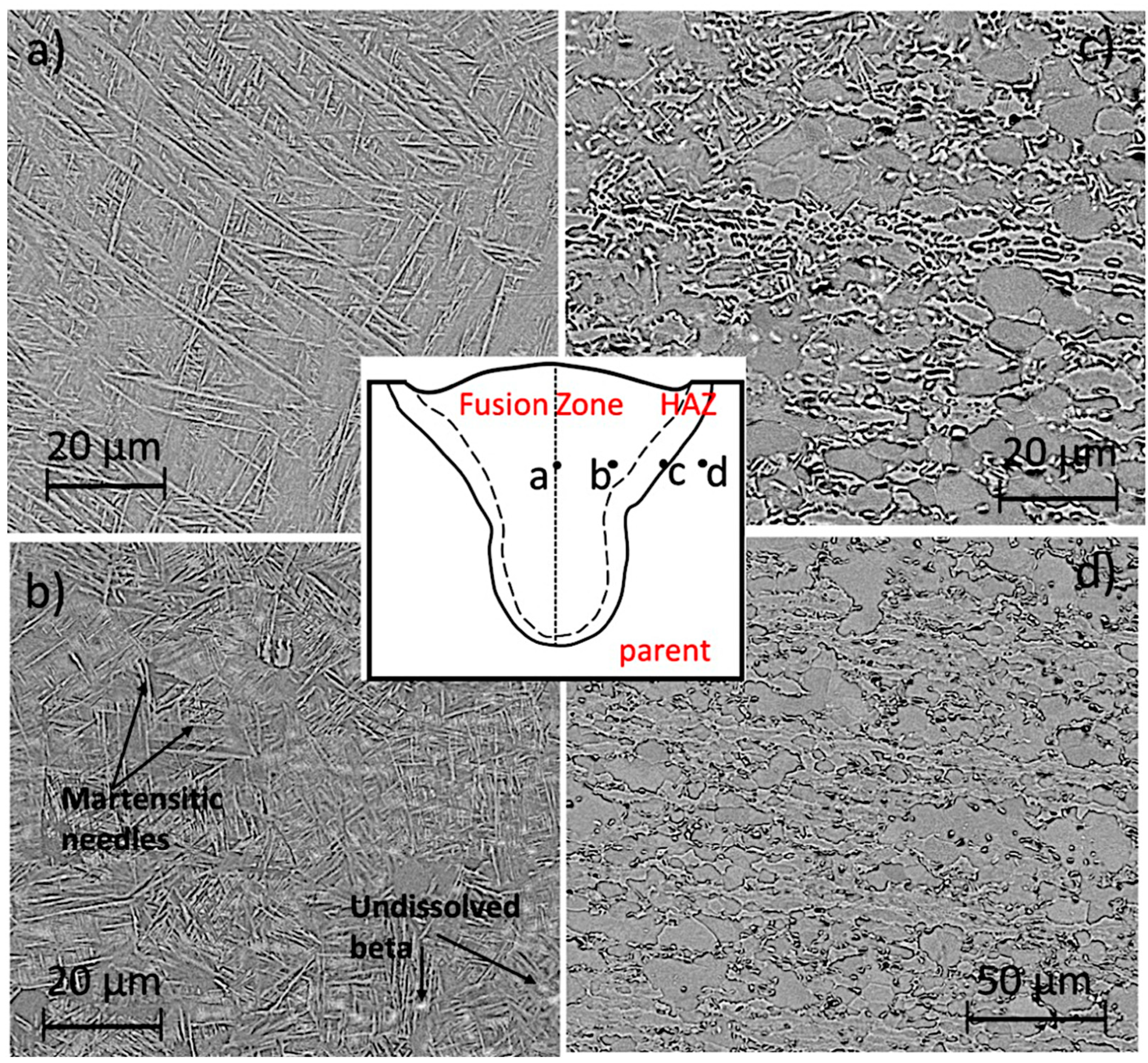
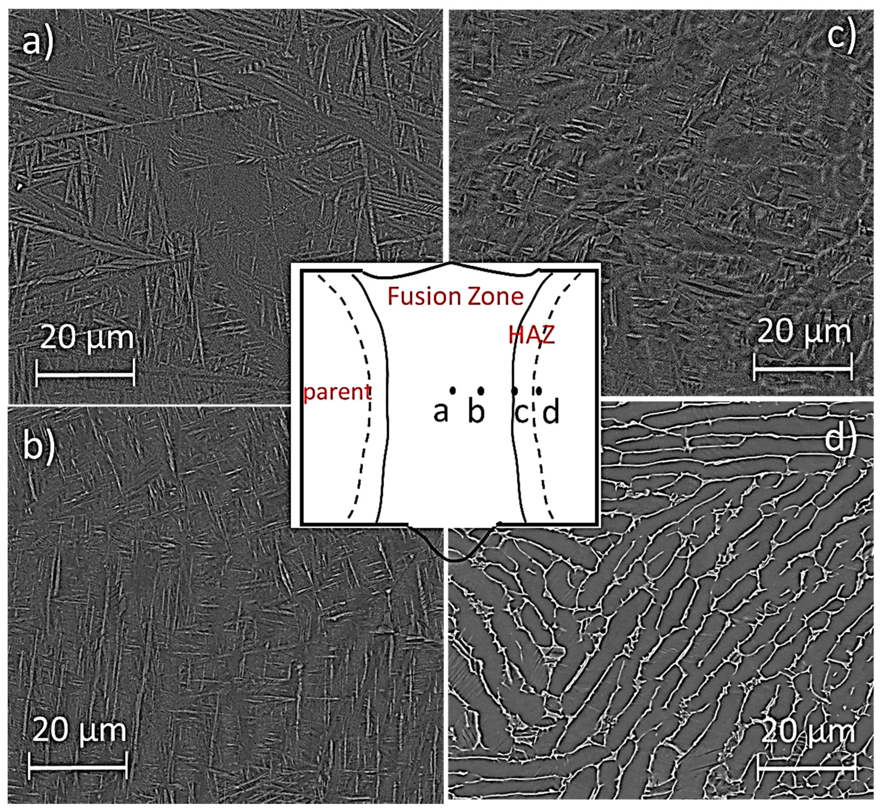
3. Results—Microstructure Characterisation

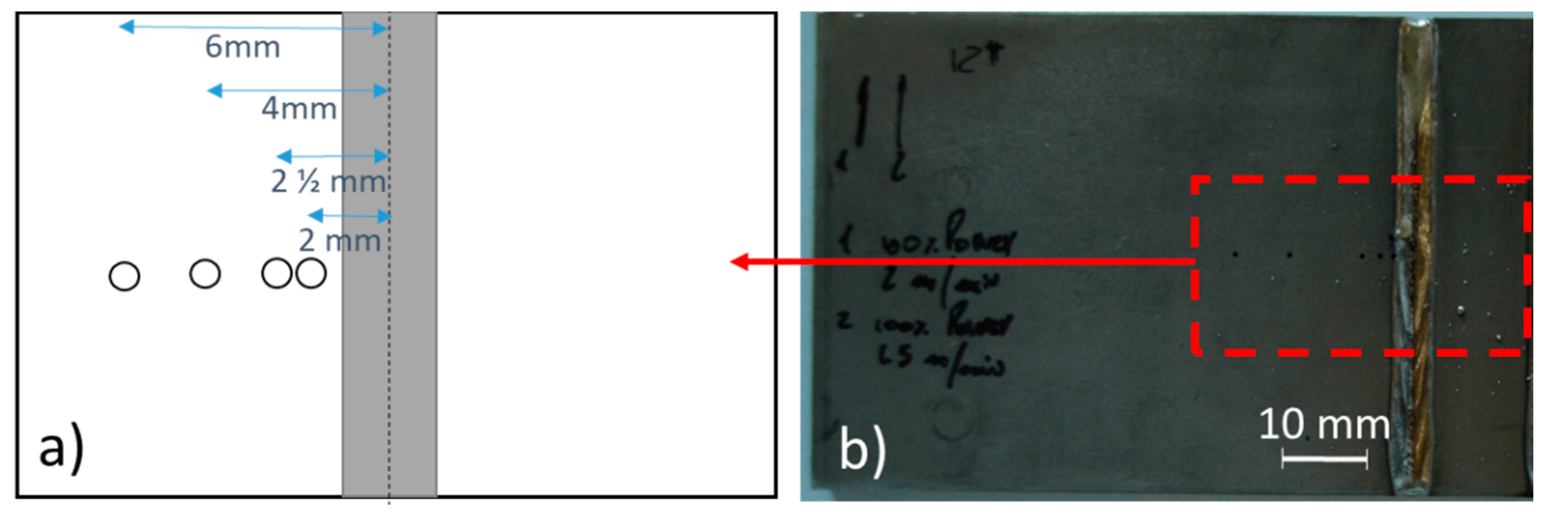
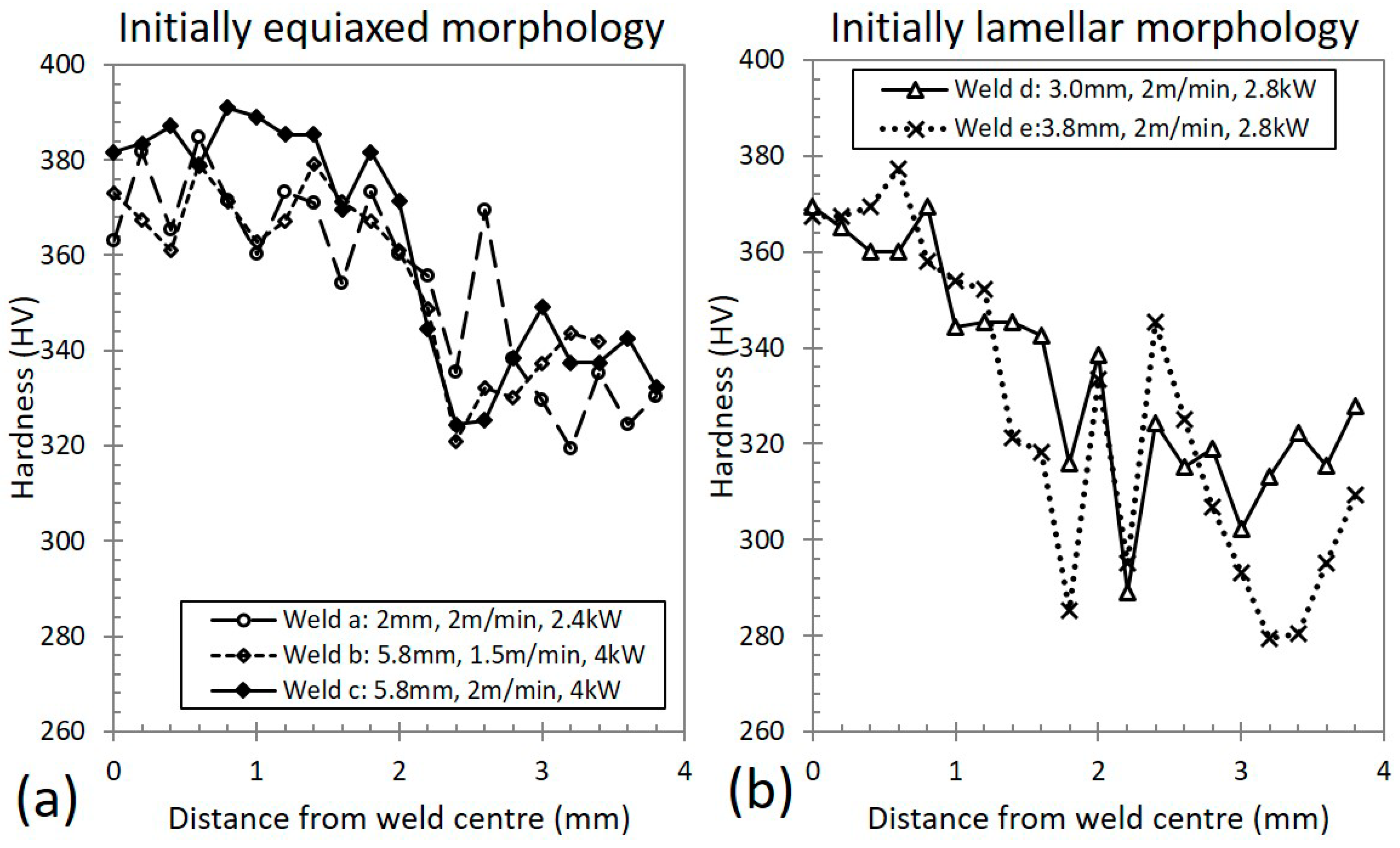
3.1. Weld Pool Imaging and Hardness Measurements

To study the microstructures, a series of microindentations using a hardness machine allowed for the measurement of the hardness of the material at different locations and marking of location references at which to take BEI images using an Oxford Instrument XL30 ESEM EG (Zeiss, Oberkochen, Germany). Images at larger scale were obtained using a Zeiss Axioskop 2 MAT microscope with AxioVision software v 4.6.3.0 (Zeiss, Oberkochen, Germany). The analysed samples were prepared by polishing and etching in a 2% HF and 10% HNO₃ solution. Microstructure measurements were carried out following a procedure described in the literature [19].

The micrographs shown in Figure 3a–c correspond to the weld zones of the equiaxed microstructure plates, while Figure 3d,e corresponds to the lamellar microstructure plates. For the equiaxed plate, it is evident that at higher weld speeds, the energy passing into the plate per unit length is lower, thus resulting in less penetration of the weld bead. Some porosity can be observed, possibly due to the formation of gas bubbles. The holes used to fix the thermocouples are visible and the influence of these holes on the shape of the weld pool can be noted by comparison of the right side to the left. The resulting weld pool shapes for the plates with an initial lamellar grain morphology were very similar to the fully penetrating 5.8-mm-thick, 1.5 m min⁻¹ weld, with a classical hourglass bead cross-sectional shape.

A β columnar morphology can be observed in the centre of all the microstructures shown, with an orientation going from the heat-affected zone, where the first β nuclei formed from colder material, toward the centre, where the hottest part of the material is. These columnar grains, looking in the centre line of the weld pool, are also oriented toward the colder side—in the upper side they grow upward, in the bottom side they grow downward. In the centre, the elongated β columnar microstructure becomes more equiaxed.

Microhardness measurements were taken on the side unaffected by the presence of thermocouple holes. The hardness measurements were taken along the dotted lines indicated on each micrograph in Figure 3. The hardness measurements for the plate welds with equiaxed and lamellar morphologies are reported in Figure 4a,b. The point at which the measurements start is indicated with a red arrow in Figure 3, and the indents are spaced incrementally at steps of 0.2 mm, moving perpendicularly away from the weld centre. The location of the interface between the HAZ and parent material along the line chosen for hardness measurements is indicated by the white arrow in Figure 3.

Similar to the findings in the literature [31], in Figure 4 above, the microhardness for the initially equiaxed plates is higher in the fusion zone (370 HV) than the parent zone (330 HV), since a martensitic microstructure is developed during cooling from the welding process. For the plates with an initially lamellar morphology, the material is harder in the fusion zone than the parent because of the martensitic microstructure. Compared with the equiaxed plate, the hardness values measured in the weld pool of the lamellar morphology plate are very similar (peaking at 370–380 HV), whilst in the bulk material there is a considerable difference, with the equiaxed parent microstructure having a higher hardness (330–340 HV) than the material with the lamellar parent microstructure (300–310 Vickers). The two initially lamellar plates have similar hardness values, suggesting that the difference in thickness is within the range that does not cause significant variation in the gradient of temperatures in the specimens during welding or that causes substantially different microstructures to develop with different mechanical responses.

It is also interesting to note that the oscillation in the measured microhardness in the fusion zone measurements for the initially equiaxed morphology plates, particularly for the 2-mm-thick plate and the 5.8-mm-thick plate with 2.0 m min⁻¹ weld speed, was likely caused by regions with different grain orientations. The 5.8-mm-thick plate welded at a speed of 2 m min⁻¹ appeared to have a slightly higher hardness in the fusion zone than the same thickness plate welded at the slower speed. This was likely caused by the higher cooling rate of the material being welded at a faster speed, meaning a fully martensitic structure developed, whilst the material welded at speeds slower produced both martensite and lamellar microstructures in the fusion zone upon cooling (Figure 5b,c). For the two plates with an initially lamellar morphology (Figure 5d–e), the weld microstructure was very similar at the centre of the fusion zone.

Even though the geometry and thermal load were very different, the 2-mm-thick plate showed a hardness in the fusion zone similar to that of the 5 mm plate welded at 1.5 m/min. Comparing the microstructures in the fusion zones for these two welds (Figure 5a,c), there were similarities regarding the presence of both lamellar and martensitic structures. This highlights the critical relationship between microstructure and mechanical properties within the material. Further observation illustrated a drop in hardness close to the interface between the parent material and the heat-affected zone (HAZ; approximately 2.3 mm away from weld centre), which was possibly caused by the effect of releasing local residual stresses in the parent microstructure [32]. In this narrow area, the heating induced by the welding process increased the temperature to values sufficient for annealing but not high enough to generate harder lamellar or martensitic microstructures.

The slightly different chemical compositions of the plates were assumed to have a relatively low impact on the hardness of the welded zone, as no relevant variation of the hardness was measured in any of the plates tested. In the bulk material, appreciable differences in hardness measurements were encountered (see Figure 4), suggesting that the different compositions and processing routes associated with the equiaxed and lamellar microstructures gave rise to the variations in hardness and mechanical properties.

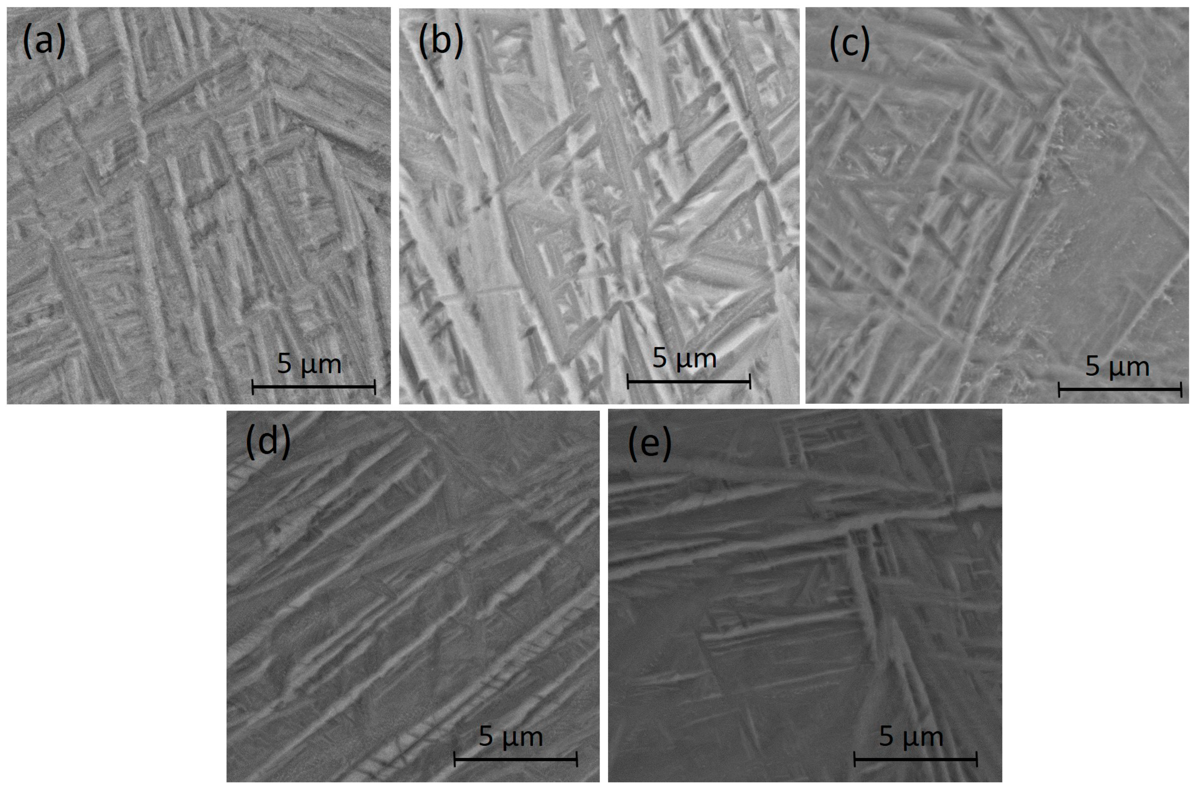
3.2. Microstructure of the Initially Equiaxed Plates

The 5.8 mm equiaxed plate welded at 2 m min⁻¹ was analysed using backscattered SEM imaging at locations moving progressively away from the centre of the weld pool, which revealed how the microstructure evolved with the changing temperature (Figure 6). Starting in the parent microstructure (Figure 6d), the original white β particles dissolved gradually (Figure 6d–b) and remained visible in areas where new β grains were nucleating.

Figure 6 demonstrates how vanadium, which segregates into the β precipitates, diffuses through the matrix slower than aluminium, and as such is considered the controlling diffusing element in the numerical model. The presence of residual localised segregation related to the parent equiaxed α precipitates, e.g., martensite needles, can also be noted in Figure 6b, implying that even if the overall tendency of the crystallographic structure of the material is to switch from HCP to BCC, the diffusing elements are limited in their speed by the diffusion process. Lastly, comparing Figure 6b to Figure 6a, moving toward the centre of the weld pool, the β grains become larger as the cooling rates are lower in central locations. The length of the transformed β needles also increases as the β grains grow.

3.3. Microstructure of the Initially Lamellar Plates

The 3.8 mm plate with an initially lamellar morphology welded at 2 m min⁻¹ was analysed using backscattered SEM imaging at locations moving progressively away from the centre of the weld pool. This revealed how the microstructure evolved with the changes of temperature. Starting in the parent material and moving inwards, in Figure 7d it is possible to observe the gradual dissolution of the original lamellar microstructure as the white β boundaries thicken and the dark α areas thin. Simultaneously, as the temperature reaches above β-transus and upon subsequent cooling, new lamellae started to nucleate and grow (Figure 7c), then with further temperature increases martensitic needles formed (Figure 7a,b). The speed of the welding process allowed insufficient time for homogenisation of the different chemical species in the constituent α and β phases; thus, in some locations where the temperature exceeds the β-transus, one can observe local segregation, as seen in the light and dark areas in Figure 7c, representing positions very close to the weld pool fusion zone.

Simultaneously, as the temperature reached above β-transus and upon subsequent cooling, new lamellae started to nucleate and grow (Figure 7c), then with further temperature increases martensitic needles formed (Figure 7a,b). The speed of the welding process allowed insufficient time for homogenisation of the different chemical species in the constituent α and β phases; thus, in some locations where temperature exceeds the β-transus, one can observe local segregation, as seen in the light and dark areas in Figure 7c, representing positions very close to the weld pool fusion zone.

3.4. Lamellar Thickness and Equiaxed Grain Size

For the initially equiaxed plates, the post-welding thickness of the lamellae and the radius of the spherical α precipitates are illustrated as a function of the distance from the centre of the weld pool (Figure 8a,b). The lamellae widths post-welding for the initially lamellar morphology are presented in Figure 9a,b.

At locations closer to the weld path, the original equiaxed microstructure vanished progressively, giving rise to the lamellar microstructure from the formed β phase. The thickness of the nucleated lamellae increased toward the centre of the weld, possibly caused by the increasing size of the β grains in the areas where they nucleated, which in turn was associated with the higher temperature to which the material was subjected.

As observed previously, the lamellae thickness in the 5 mm plate welded at 1.5 m min⁻¹ was similar to the lamellae thickness that developed in the 2 mm plate welded at 2.0 m min⁻¹, which resulted in similar hardness measurements in the fusion zones for these 2 welds. The evolution of the original lamellae thickness for the plates with an initially lamellar morphology tended to become when smaller moving toward the higher temperatures closer to the centre of the weld pool (see Figure 9a). The thickness of the nucleated lamellae seemed to be influenced by the thickness of the plate, as thicker plates had thicker nucleated lamellae, possibly caused by the marginally slower heat loss through the different specimen thicknesses (3.0 and 3.8 mm) (see Figure 9b).

3.5. Chemical Analysis

The chemical compositions (wt%) for the initially equiaxed 5.8 mm plate welded at 2.0 m min⁻¹ and 4.0 kW and for the initially lamellar 3.8 mm plate welded at 2.0 m.min⁻¹ and 2.8 kW are reported as functions of the distance from the weld line (Figure 10). The high variation in the vanadium contents of the β phase is evident. This was due to the speed of the welding process preventing the homogenisation of the chemical segregation present in the phases in the initial material. The effect of the chemical composition of the phases present in the parent microstructure was still noticeable after the formation of new morphological features, such as α lamellae or martensitic needles. This local segregation phenomenon is shown in Figure 10.

4. Finite Element Modelling

The numerical microstructure models developed previously by Villa et al. [16,17] were coded into subroutines within the commercial software Sysweld (by ESI-Group) in order to run weld simulations capable of predicting the microstructural evolution of the material during the joining process. This metallurgical framework is based upon physics-based models for temperatures within the α+β field and the Johnson–Mehl–Avrami (JMA) approach, which is used extensively in the literature to simulate phase transformations [16,17,18,28] for temperatures above the beta transus temperature. Appropriate element sizes were used, such that smaller brick elements caused no significant changes to the results. The modelled outputs, which were visible in the post-processor at each time step of every integration point, included volume fractions of the (i) equiaxed α phase, (ii) lamellar α phase, (iii) β phase, and (iv) martensitic α’ phase, as well as the sizes of the equiaxed α mean radius, lamellar α thickness, α’ needle thickness, and β grain radius. The main equations used to describe the particle size evolution are reported here as Equations (1)–(12); the reader is directed to [18,19] for a thorough analysis of the mathematical framework for these equations and values.

Growth of spherical particles:

$$\frac{dR}{dt}=2{\lambda }^2\frac{D}{r}$$

(1)

Shrinkage of spherical particles:

$$\frac{dR}{dt}=\frac{\mathsf{\Omega }\mathrm{D}}{4R}+\frac{\mathsf{\Omega }}{4}\sqrt{\frac{D}{\pi t}}$$

(2)

Volume fraction of α spherical particles:

$$f_{\alpha s}=f_{\alpha s0}\left(\frac{R_{\propto s}}{R_{\alpha s0}}\right)$$

(3)

Growth of lamellar α phase particles:

$$Y=2\Gamma {\left(\delta Dt\right)}^{\frac{1}{2}}$$

(4)

$$X=2{\left(\delta Dt\right)}^{\frac{1}{2}}$$

(5)

Shrinkage of lamellar α phase:

$$S=S_0-{\lambda }_1{\left(Dt\right)}^{\frac{1}{2}}$$

(6)

Volume of lamellar α particles:

$$\frac{d{V}_e}{dt}=8\pi {\Gamma }^2\delta DX$$

(7)

The β grain growth:

$$d_{\beta }^n-d_{\beta 0}^n=A\times t\times e^{-\left(\frac{Q}{R{T}_2}\right)}$$

(8)

The β volume fraction:

$$f_{\beta }=f_{\beta 0}\left(\frac{R_{\beta }}{R_{\beta 0}}\right)$$

(9)

Nucleated α lamellae thickness:

$$S=-0.0013\left(\frac{dt}{dt}\right)+0.0787\ln d$$

(10)

Martensitic needles thickness:

$$S^{\prime }=0.0895\ln \left(\frac{dT}{dt}\right)-0.138$$

(11)

Martensitic volume fraction:

$$f{\alpha }^{\prime }=20.4\times \left(2.62+{\tan }^{-1}\left\{\left[\frac{dT}{dt}\right]-65\right\}\right)$$

(12)

where R_αs is the radius of the α spherical particles, R_αs0 the initial radius of α spherical particles, λ is a function of the supersaturation term Ω, D is the inter-diffusion coefficient, f_αs0 is the initial α volume fraction of spherical particles, f_αs is the α volume fraction of spherical particles, Y is the major length of the ellipse, X is the minor length of the ellipse, Γ is the aspect ratio given by Y/X, δ is the dimensionless growth parameter, S is the lamellae thickness, S₀ is the initial lamellae thickness, λ₁ is the parameter of the supersaturation equation for lamellae shrinkage, V_e is the volume of the lamellar α particle, d_β is the diameter of the β grains, R_β is the radius of the β grains, A and n are material-specific constants, R is the gas constant, Q is the activation energy for grain growth, T₂ is a correction factor, f_β is the β volume fraction, and f_α’ is the martensitic volume fraction.

To validate the predictions of the welding simulations, the results were compared with the data obtained from the experimental welding tests. The thermal properties of the material used for the numerical simulations were estimated using the values given in the literature for thermal conductivity [32,33,34], specific heat [33,35,36], and density [34,36,37], which were obtained from several sources. For numerical stability, the peak of the specific heat corresponding to the liquidus temperature was scaled over a larger range of temperatures, whilst keeping the area representing the latent melting heat constant. The plate was meshed using the meshing module of the FE software, using 3D brick linear elements measuring ~0.2 mm × 0.2 mm × 0.2 mm close to the weld line. A higher element density close to the area of the weld pool was used to decrease the temperature gradient for the elements subjected to very high variations of temperature over space and time. Far from the weld pool, the number of elements representing the thickness of the model was six, as this value is the limit at which linear elements can correctly represent the bending of thin plates [38]. For the thickest plate measuring 5.8 mm, this corresponded to 201,520 elements.

The boundary conditions in the model were applied to the plates (clamped only on the left side) in the same way as in the experiments. All of the external surfaces were set to be in contact with air at 40 °C, as this was the temperature measured at the end of the welding tests. In reality, this temperature changes during welding tests; however, for simplification it was assumed to be constant. The convection coefficient was assumed as a function of the temperature, with a value of 20 W m⁻¹K⁻¹ at ambient temperature, which increased asymptotically to 30 m⁻¹K⁻¹. The emissivity was assumed to be constant at 0.8.

For the modelling of the phenomena occurring in the weld pool, a classical approach to computational welding mechanics using a modified Gaussian heat source was adopted [39]. This approach requires the determination of the weld pool shape using experimental measurements and fitting of the numerical heat source to the measured heat source by adjusting the heat flow distribution in 3D space. The welding experiments were, thus, executed before the simulations, then the welds were sectioned and the weld pool width was recorded as a function of the depth. This heat source model is presented in the literature [40]. Weld pool dimensions for the models were matched to the experiment.

5. Calibration and Validation

5.1. Calibration of Thermal Data

A comparison of the FE-generated weld pool, which was calibrated using the weld pool width as a function of depth with Cartesian coordinates, against the experimentally observed welds using a method described previously in the literature [29,39,40] is presented in Figure 11. For all welds modelled in this study, the numerical software reconstruction of the calibrated weld pool shape was considered to satisfactorily match the experiment when the boundary of the fusion zone was predicted within a tolerance of ±0.1 mm.

Further thermal calibration and analysis of the numerical model were carried out by comparing the temperatures predicted at different distances from the weld trajectory with the ones measured by the thermocouples in the experiments. The temperatures measured in the numerical simulations were relatively sensitive to the thermal properties adopted to model the material behaviour, and to a lesser degree also to the temperature surrounding the workpieces and the convection coefficient. A comparison of thermal predictions versus experimental results for the 3.0 mm plate with an initially lamellar morphology is shown in Figure 12. The temperatures reported for the numerical model reference the closest node in the mesh in order to match the locations of the thermocouple tips, which were positioned at the base of each channel.

For both equiaxed and lamellar plates, a good match between the numerical and experimental results was obtained, in particular for the locations closest to the weld line, where the temperatures were high enough to affect the material microstructure over the typical timings involved during welding. The slightly higher temperatures predicted by the numerical model compared with the experiment far from the weld line were hypothesised to be caused by (a) the influence of the convection coefficient at lower temperatures and (b) local effects of thermal inertia caused by the presence of thermocouple wires in the experiment. Considering the complexity of the experimental setup, the reasonable match between the numerical models and experimental results suggests that the model made sensible assumptions for boundary conditions and material properties [29,39]. The good matching of the predicted and observed weld pool shapes and further analysis of the temperature trends will ensure that the microstructure models refer to appropriate thermal data.

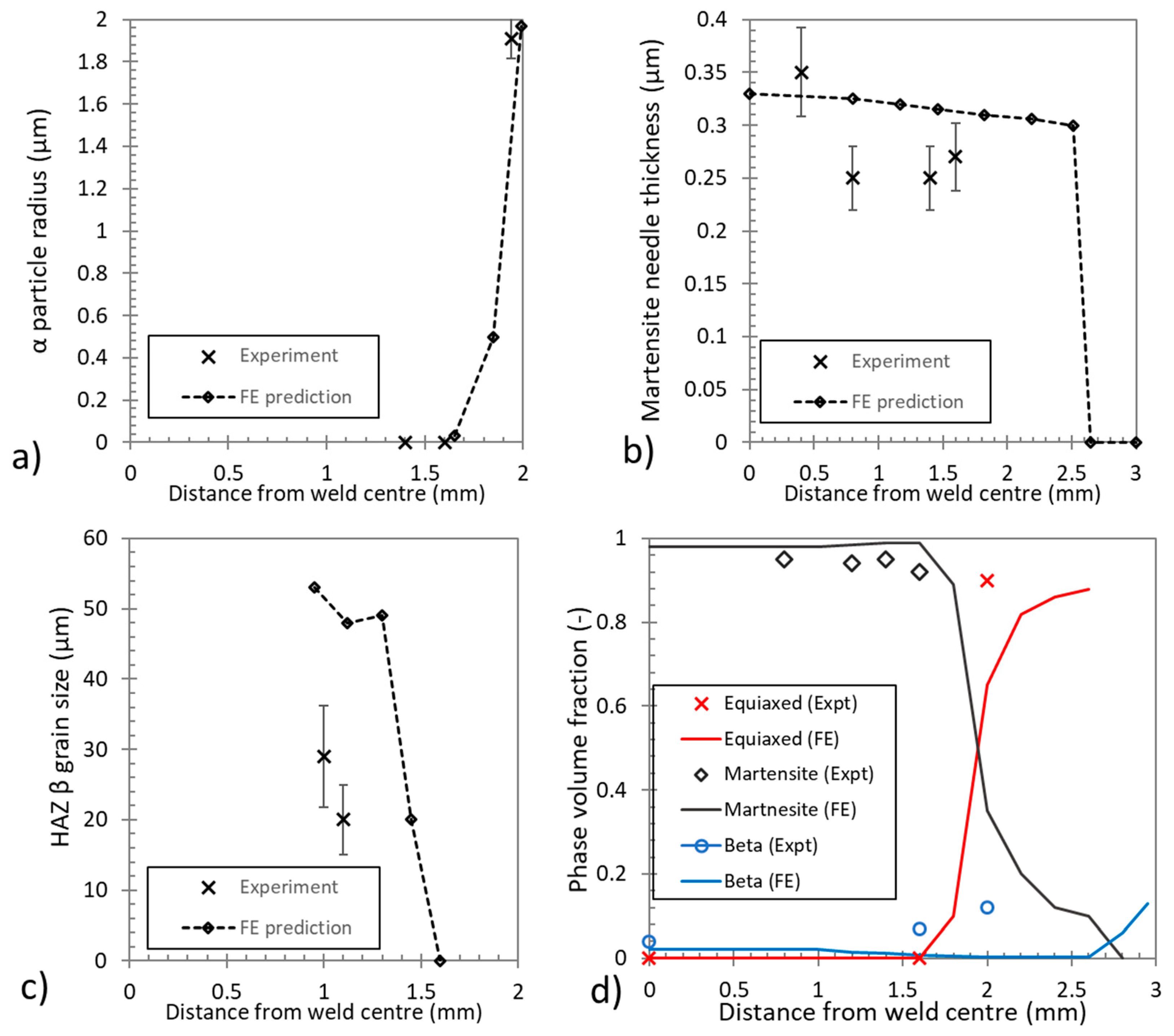
5.2. Plates with an Initially Equiaxed Microstructure

The experimental measurement of microstructural features was not always easy, particularly when many topologies of phases and particles were present in the same SEM image. The metallurgical model, when embedded in to the welding FE code, was validated for the prediction of the (a) mean radius of the equiaxed α phase, (b) mean martensitic needles thickness, (c) β grain radius in the HAZ, and (d) phase volume fractions. The resulting FE–metallurgy coupled modelling predictions and experimental measurements from the 2.0-mm-thick plate with an initially equiaxed microstructure are shown as functions of the distance from the weld line in Figure 13a–d. A good match between numerical prediction and experimental results was obtained for the α particle size (Figure 13a), accurately capturing the distance from the weld line where the α particles dissolve. A relatively good match between the numerical prediction and experimental results was obtained for the martensitic needle thickness (Figure 13b). Although the FE model gave needle thickness predictions up to 2.6 mm, since SEM images were taken only up to a distance of 1.7 mm, validation beyond this location was not possible.

The numerical model for HAZ β grain growth appeared to miss the correct distance from the weld for β grains of a particular size, with an error of about 0.3–0.4 mm (Figure 13c). Since the β grain nucleation temperature for the initially equiaxed morphology was not investigated experimentally, the same temperature as for the initial lamellar microstructure was assumed. The results suggested that the nucleation temperature of the initially equiaxed microstructure was higher than that for the lamellar microstructure. A comparison between the equiaxed α and martensitic and β phase proportions is presented in Figure 13d. The numerical predictions match reasonably well with the experimental results for SEM images up to 2.0 mm from the weld line. For the β phase fraction prediction, although it does not fit than the other phases, it is still within the experimental error range.

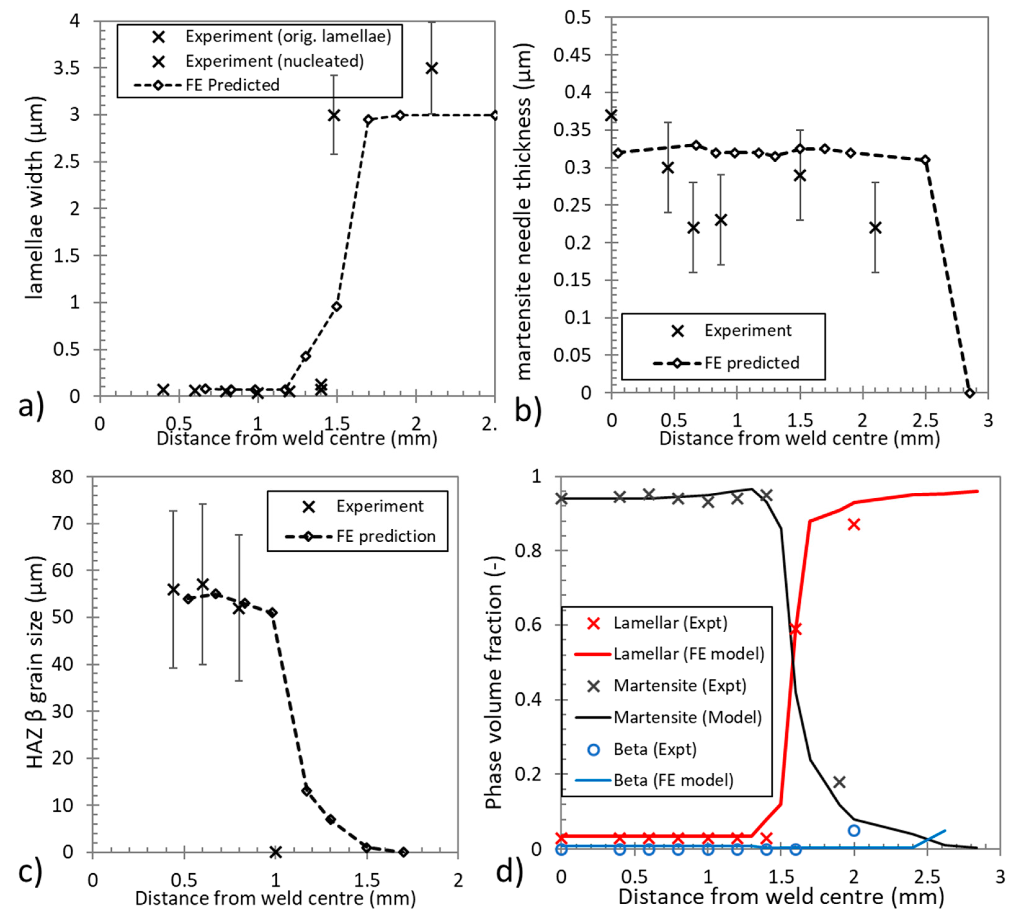
5.3. Plates with an Initially Lamellar Microstructure

The resulting FE–metallurgical modelling predictions for the (a) mean radius of the equiaxed α phase, (b) mean martensitic needles thickness, (c) β grain radius in the HAZ, and (d) phase volume fractions were computed and assessed. These results were compared with experimental measurements for these features from the 3.0-mm-thick plate with an initial lamellar microstructure and are shown as functions of the distance from the weld line. In Figure 14a, the original lamellar thickness of the microstructure and the thickness of nucleated lamellae are differentiated in the experimental data, as they were recognizable experimentally. Considering the possible experimental errors in the different measurements taken during SEM analysis, regarding the measured weld pool size and FE modelling tolerance (0.1 mm), a good match between the numerical and experimental results was obtained, capturing the transition between the disappearance of the original lamellae and the nucleation of new lamellae.

Figure 14b compares the numerical model and experimental measurements of the mean martensitic needles thickness as functions of the distance away from the weld. Some of the numerical predictions are in reasonable agreement with the experimental measurements, however for the furthest locations from the weld line, the numerical model seems to overpredict the areas where martensitic needles stop forming by about 0.5–1.0 mm. These errors in the modelled results imply that the conditions for martensite formation in the current model, which were deduced from the cooling rate [19] and the literature [41], should be reconsidered. The martensitic needle model assumes a minimum cooling rate of 30 °C/s and a martensite temperature range of 700–800 °C. This suggests that either a higher minimum cooling rate or range of temperatures should be adopted.

Figure 14c compares the numerical model and experimental measurements of the mean β grain radius dimension in the HAZ as functions of the distance away from the weld. The FE numerical model assesses the temperature and time at that temperature to indicate the nucleation of β grains. The β-transus temperature was assumed to be passed when a martensitic microstructure was observed within parent α lamellae at the end of the heat treatments, whilst the lowest temperature at which β grains were noticed for a specific heating rate was assumed as the nucleation temperature of the β grains. Errors in the predictions of the β grain size were hypothesised to be caused by four factors, namely the weld pool width differences between the experiment and the model, the bigger area sampled experimentally (0.2 × 0.2 mm²) than the corresponding numerical model mesh size of this location (0.156 × 0.156 mm²), the combination of relatively large β grains mixed with neighbouring smaller grains experimentally observed here, and lastly the influence experimentally of mechanical impingement of neighbouring β grains, which was not included in the model. Thus, the numerical model may represent the area as containing larger β grains, whilst neglecting small neighbouring grains, which would reduce the mean β grain size.

The FE–metallurgical numerical model predictions of the phase fractions of the lamellar phase, martensite phase, and β phase shown in Figure 14d are generally in good agreement with the experiments. However, when simulating the initially equiaxed microstructure, the code slightly underpredicted the β phase and overpredicted the martensite phase. For the code simulating the initially lamellar plate, this consistently under predicted the lamellar, martensite, and β phases. The largest errors occurred in predictions furthest from the weld line for all three phases, particularly the martensite and β phases. These errors may have been due to conditions assumed within the model for the martensitic transformation to occur.

6. Conclusions

A computational methodology for coupling previously established metallurgical models was presented, which was based upon the JMA method and a diffusion-based approach and which describes the microstructure evolution of Ti-6Al-4V alloys within a commercially available FE welding code. A comparison between experimental and numerical results conducted on plates with either initially equiaxed or lamellar microstructures led to the following conclusions:

• The microstructural model predictions are in good agreement with the structural characterisation results obtained from the test welds. The increase in welding simulation run times obtained when adopting the models developed in this work was roughly 100% when compared to those for the conventional approach adopted in the welding FE code;
• The diffusion-based approach, which was previously developed and validated, can be adopted to describe the microstructure evolution within the α+β field in welding processes. The diffusion-based model is accurate and is based only on fundamental material properties; thus, once the initial chemical composition and particle dimensions of the material are known, the model is ready for both equiaxed and lamellar microstructures;
• There is considerable potential for further refinement of this approach for use by welding engineers. Further studies to extend this physics-based approach to the full range of temperatures that occur during welding is desirable. This would cause longer computational times but would require no further calibration experiments;
• The microstructural evolution of the particle dimensions was successfully predicted, which is important for mechanical strength predictions of titanium alloys and for possible future fatigue life modelling.

References

1. Boyer, R.R. An overview on the use of titanium in the aerospace industry. Mater. Sci. Eng. A 1996, 213, 103–114. [Google Scholar] [CrossRef]
2. Mendez, P.F.; Eagar, T.W. Welding Processes for Aeronautics. Adv. Mater. Process. 2001, 5, 39–43. [Google Scholar]
3. Haque, R. Quality of self-piercing riveting (SPR) joints from cross-sectional perspective: A review. Arch. Civ. Mech. Eng. 2018, 18, 83–93. [Google Scholar] [CrossRef]
4. Galinska, A.; Galinski, C. Mechanical Joining of Fibre Reinforced Polymer Composites to Metals—A Review. Part II: Riveting, Clinching, Non-Adhesive Form-Locked Joints, Pin and Loop Joining. Polymers 2020, 12, 1681. [Google Scholar] [CrossRef] [PubMed]
5. Pederson, R. Microstructure and Phase Transformation of Ti-6Al-4V. Ph.D. Thesis, Lulea University, Luleå, Sweden, 2002. [Google Scholar]
6. Lopez de Lacalle, L.N.; Sanchez, J.A.; Lamkiz, A.; Celaya, A. Plasma Assisted Milling of Heat-Resistant Superalloys. ASME J. Manuf. Sci. Eng. 2004, 126, 274–285. [Google Scholar] [CrossRef]
7. Avrami, M. Kinetics of Phase Change, I—General Theory. J. Chem. Phys. 1939, 7, 1103–1112. [Google Scholar] [CrossRef]
8. Avrami, M. Kinetics of Phase Change, II—Transformation—Time relations. J. Chem. Phys. 1940, 8, 212–224. [Google Scholar] [CrossRef]
9. Avrami, M. Kinetics of Phase Change. III—Granulation, Phase Change, and Microstructure. J. Chem. Phys. 1941, 9, 177–184. [Google Scholar] [CrossRef]
10. ESI-Group. Sysweld 2013 Reference Manual; ESI-Group: Lyon, France, 2012. [Google Scholar]
11. Ding, R.; Guo, Z.X.; Wilson, A. Microstructural evolution of Ti–6Al–4V alloy during thermomechanical processing. Mater. Sci. Eng. A 2002, 327, 233–245. [Google Scholar] [CrossRef]
12. Gil, F.J.; Manero, J.M.; Ginebra, M.P.; Planell, J.A. The effect of cooling rate on the cyclic deformation of β-annealed Ti–6Al–4V. Mater. Des. 2003, 349, 150–155. [Google Scholar] [CrossRef]
13. Tiley, J.; Searles, T.; Lee, E.; Kar, S.; Banerjee, R.; Russ, J.; Fraser, H. Quantification of microstructural features in α/β titanium alloys. Mater. Sci. Eng. A 2004, 372, 191–198. [Google Scholar] [CrossRef]
14. Mi, G.; Wei, Y.; Zhan, X.; Gu, C.; Yu, F. A coupled thermal and metallurgical model for welding simulation of Ti–6Al–4V alloy. J. Mat. Proc. Technol. 2014, 214, 2434–2443. [Google Scholar] [CrossRef]
15. Fan, Y.; Cheng, P.; Yao, Y.L.; Yang, Z.; Egland, K. Effect of phase transformations on laser forming of Ti–6Al–4V alloy. J. Appl. Phys. 2005, 98, 1–10. [Google Scholar] [CrossRef]
16. Malinov, S.; Guo, Z.; Sha, W.; Wilson, A. Differential scanning calorimetry study and computer modeling of β ⇒ α phase transformation in a Ti-6Al-4V alloy. Metall. Mater. Trans. A 2000, 32A, 879–887. [Google Scholar] [CrossRef]
17. Katzarov, I.; Malinov, S.; Sha, W. Finite element modeling of the morphology of β to α phase transformation in Ti-6Al-4V alloy. Metall. Mater. Trans. A 2001, 33A, 1027–1040. [Google Scholar] [CrossRef]
18. Villa, M.; Brooks, J.; Turner, R.P.; Wang, H.; Boitout, F.; Ward, R.M. Microstructural Modeling of the α + β Phase in Ti-6Al-4V: A Diffusion-Based Approach. Metall. Mater. Trans. B 2019, 50, 2898–2911. [Google Scholar] [CrossRef] [Green Version]
19. Villa, M.; Brooks, J.; Turner, R.P.; Boitout, F.; Ward, R.M. Microstructural Modeling of Thermally-Driven β Grain Growth, Lamellae & Martensite in Ti-6Al-4V. Modeling Numer. Simul. Mater. Sci. 2020, 10, 55–73. [Google Scholar]
20. Semiatin, S.L. An Overview of the Thermomechanical Processing of α/β Titanium Alloys: Current Status and Future Research Opportunities. Metall. Mater. Trans. A 2020, 51A, 2593–2625. [Google Scholar] [CrossRef] [Green Version]
21. Gil, F.J.; Ginebra, M.P.; Manero, J.M.; Planell, J.A. Formation of α-Widmanstätten structure: Effects of grain size and cooling rate on the Widmanstätten morphologies and on the mechanical properties in Ti6Al4V alloy. J. Alloys Compd. 2001, 329, 142–152. [Google Scholar] [CrossRef]
22. Kempf, J.M.; Gautier, E.; Simon, A.; Uginet, J.F.; Gavart, A. Titanium ’92: Science and Technology; Froes, F.H., Caplan, I.L., Eds.; TMS: Warrendale, PA, USA, 1993; pp. 627–634. [Google Scholar]
23. Allan, M.; Thomas, M.; Brooks, J.; Blackwell, P. β Recrystallisation Characteristics of α + β Titanium Alloys for Aerospace Applications. In Proceedings of the 13th World Conference on Titanium, San Diego, CA, USA, 16–30 August 2015; Venkatesh, V., Pilchak, A.L., Allison, J.E., Ankem, S., Boyer, R., Christodoulou, J., Fraser, H.L., Imam, M.A., Kosaka, Y., Rack, H.J., et al., Eds.; TMS: Warrandale, PA, USA, 2016; pp. 203–208. [Google Scholar]
24. Ivasishin, O.M.; Shevchenko, S.V.; Semiatin, S.L. Effect of crystallographic texture on the isothermal β grain-growth kinetics of Ti–6Al–4V. Mater. Sci. Eng. A 2002, A332, 343–350. [Google Scholar] [CrossRef]
25. Konovalov, S.; Komissarova, I.; Ivanov, Y.; Gromov, V.; Kosinov, D. Structural and phase changes under electropulse treatment of fatigue-loaded titanium alloy VT1-0. J. Mater. Res. Technol. 2019, 8, 1300–1307. [Google Scholar] [CrossRef]
26. De Jesus, J.; Ferreira, J.A.M.; Borrego, L.; Costa, J.D.; Capela, C. Fatigue Failure from Inner Surfaces of Additive Manufactured Ti-6Al-4V Components. Materials 2021, 14, 737. [Google Scholar] [CrossRef]
27. Xia, J.; Jin, H. Numerical modeling of coupling thermal–metallurgical transformation phenomena of structural steel in the welding process. Adv. Eng. Softw. 2018, 115, 66–74. [Google Scholar] [CrossRef]
28. Jones, S.J.; Bhadeshia, H.K.D.H. Kinetics of the simultaneous decomposition of Austenite in to several transformation products. Acta Mater. 1996, 45, 2911–2920. [Google Scholar] [CrossRef]
29. Lindgren, L.-E. Computational Welding Mechanics Thermomechanical and Microstructural Simulations; Woodhead Publishing: Cambridge, UK; Maney Publishing: Leeds, UK, 2007. [Google Scholar]
30. Anderson, R.L. Thermocouple Error Analysis in the Design of Large Engineered Experiments. Oak Ridge National Labs. Internal Report. 1979. Available online: https://www.osti.gov/servlets/purl/12104847 (accessed on 15 March 2021).
31. Squillace, A.; Prisco, U.; Ciliberto, S.; Astarita, A. Influence of Welding Parameters and Post-weld Aging on Tensile Properties and Fracture Location of AA2139-T351 Friction-stir-welded Joints. J. Mater. Process. Technol. 2012, 212, 427–436. [Google Scholar] [CrossRef]
32. Pharr, G.M.; Tsui, T.Y.; Bolshakov, A.; Oliver, W.C. Effects of Residual Stress on the Measurement of Hardness and Elastic Modulus using Nanoindentation. MRS Proc. 1994, 338, 127. [Google Scholar] [CrossRef]
33. Boivineau, M.; Cagran, C.; Doytier, D.; Eyraud, V.; Nadal, M.H.; Wilthan, B.; Pottlacher, G. Thermophysical Properties of Solid and Liquid Ti-6Al-4V (TA6V) Alloy. Int. J. Thermophys. 2005, 27, 507–528. [Google Scholar] [CrossRef]
34. Turner, R.P.; Gebelin, J.-C.; Ward, R.M.; Reed, R.C. Linear Friction Welding of Ti-6Al-4V: Modelling and Validation. Acta Mater. 2011, 59, 3792–3803. [Google Scholar] [CrossRef]
35. Mills, K.C. Thermophysical Properties for Selected Commercial Alloys; Woodhead Publishing Ltd.: Cambridge, UK, 2002. [Google Scholar]
36. Basak, D.; Overfelt, R.A.; Wang, D. Measurement of Specific Heat Capacity and Electrical Resistivity of Industrial Alloys Using Pulse Heating Techniques. Int. J. Thermophys. 2003, 24, 1721–1733. [Google Scholar] [CrossRef]
37. Boyer, R.; Welsch, G.; Collings, E.W. Materials Properties Handbook: Titanium Alloys; ASM International: Almere, The Netherlands, 1994. [Google Scholar]
38. Villa, M. Metallurgical and Mechanical Modelling of Ti-6Al-4V for Welding Applications. Ph.D. Thesis, University of Birmingham, Birmingham, UK, 2016. [Google Scholar]
39. Goldak, J.A.; Akhlaghi, M. Computational Welding Mechanics; Springer: Berlin, Germany, 2010. [Google Scholar]
40. Turner, R.P.; Villa, M.; Sovani, Y.; Panwisawas, C.; Perumal, B.; Ward, R.M.; Brooks, J.W.; Basoalto, H.C. An Improved Method of Capturing the Surface Boundary of a Ti-6Al-4V Fusion Weld Bead for Finite Element Modeling. Metall. Mater. Trans. B 2015, 47, 485–494. [Google Scholar] [CrossRef]
41. Dabrowski, R. The Kinetics of Phase Transformations during Continuous Cooling of Ti6Al4V Alloy from the Diphase α + β Range. Arch. Metall. Mater. 2011, 56, 217–221. [Google Scholar] [CrossRef]
Figure 1. (a) Lamellar and (b) equiaxed microstructures of the Ti-6Al-4V plates.
Metals 11 00960 g001
Figure 2. (a) Schematic view of thermocouple holes and (b) photograph of the holes in relation to the weld.
Metals 11 00960 g002
Figure 3. Micrographs of sectioned weld pools for each of the instrumented welds performed (ae), the weld parameters for which are shown in Table 2.
Metals 11 00960 g003
Figure 4. Hardness profiles perpendicular to the weld pass for the plates with an (a) initially equiaxed grain morphology and (b) initially lamellar grain morphology.
Metals 11 00960 g004
Figure 5. Weld zone micrographs of various welds: (a) 2.0 mm equiaxed grain plate welded at 2.0 m min−1, 2.4 kW; (b) 5.8 mm equiaxed grain plate welded at 1.5 m min−1, 4 kW; (c) 5.8 mm equiaxed grain plate welded at 2.0 m min−1, 4 kW; (d) 3.0 mm lamellar grain plate welded at 2.0 m min−1, 2.8 kW; (e) 3.8 mm lamellar grain plate welded at 2.0 m min−1, 2.8 kW.
Metals 11 00960 g005
Figure 6. Backscattered SEM images of weld c, involving a 5.8-mm-thick equiaxed plate welded at 2 m min−1 and 4 kW for locations (ad) shown.
Metals 11 00960 g006
Figure 7. Backscattered SEM images of weld e: 3.8-mm-thick plate with a lamellar morphology welded at 2 m min−1 and 2.8 kW for locations (ad) shown.
Metals 11 00960 g007
Figure 8. The experimentally measured (a) equiaxed grain radius and (b) lamellae thickness after welding in plates with an initially equiaxed morphology.
Metals 11 00960 g008
Figure 9. The experimentally measured (a) original lamellae thickness and (b) nucleated lamellae thickness after welding in plates with an initially lamellar morphology.
Metals 11 00960 g009
Figure 10. Measured chemical compositions of (a) weld c and (b) weld e as functions of distance from the weld path.
Metals 11 00960 g010
Figure 11. FE-predicted weld pool shape for weld c using the Cartesian coordinate (width vs. depth) methodology.
Metals 11 00960 g011
Figure 12. Experimentally measured and FE-predicted thermal cycles at the specific thermocouple locations for plate weld d, which was a 3-mm-thick lamellar plate welded at 2 m min−1 and 2.8 kW.
Metals 11 00960 g012
Figure 13. FE–metallurgy coupled model predictions for weld a: (a) α radius; (b) martensite needle thickness; (c) β grain size in the HAZ; (d) phase volume fractions.
Metals 11 00960 g013
Figure 14. FE–metallurgy coupled model predictions from weld d: (a) α radius; (b) martensite needle thickness; (c) β grain size in the HAZ; (d) volume fractions of each phase.
Metals 11 00960 g014